Evaluation of Object-Space Occlusion Culling with Occluder Fusion

(1)

Evaluation of Object-Space Occlusion Culling with

Occluder Fusion

Mattias Karlsson

14 April 2011

Master Thesis in Computer Science

Advisor(s): Christian Nilsendahl, Avalanche studios

Thomas Larsson, M¨alardalens University

Examiner: Rikard Lindell, M¨alardalens University

M¨alardalens University School of Innovation, Design and

(2)

Evaluation of Object-Space Occlusion Culling with

Occluder Fusion

Abstract

In this report, an object-space solution to occluder fusion of OBB occluders is explored. Two different approaches are considered were the object-space fusion is reduced to a 2D problem. The first approach finds axis-aligned silhouettes within the projection of occluder OBBs which are then fused together creating large axis-aligned silhouettes. The other approach creates concave hulls of the projected OBB silhouettes from which convex inscribed silhouettes are then found. These silhouettes are then converted back to object-space where shadow frusta created around the silhouettes are used for the culling operation. The effectiveness of the two approaches is evaluated considering the amount of culled geometry. It is shown that fused convex silhouettes are needed to produce competitive results.

(3)

1 Occlusion culling

1.1 Background

A fundamental part of computer graphics is to determine which objects are visible and should be drawn in a scene. Algorithms addressing these problems are referred to as visibility surface determination or hidden surface removal (HSR) algorithms. Given a scene with a set of objects, the HSR algorithm need to determine not only which objects are visible but also the amount to draw of the partly hidden objects in order to produce correct images. Today, the z-buffer [3] implemented in hardware is the de-facto standard for visibility determination [5]. The z-buffer, typically a 2-dimensional buffer where each coordinate represent a pixel on screen store the depth value. Each pixel to be drawn is tested against the depth value stored at its coordinate in the z-buffer. If current pixel has lower depth value, the pixel should be displayed and the value in the z-buffer is updated with the new depth value. However, the hardware z-buffer has a severe drawback when used as the only HSR method. Because it operates late in the pipeline, all primitives have to be sent through the pipeline before they are tested for visibility. The geometry is drawn in a back to front order which is needed to produce correct images. The drawback is that every pixel in every primitive is tested against the z-buffer even if it is later overdrawn by another pixel. This is referred to as depth complexity.

1.1.1 Potential Visibility Set

Even though the z-buffer is an adequate technique to determine the final vis-ibility other algorithms are needed to reduce the depth complexity. If the set of objects sent to the rendering pipeline are reduced, the speed of the HSR can significantly be increased. This reduced subset is referred to as Potential

Visi-bility Set (PVS ) and the objective is to find a good PVS. The objects/polygons

assemble a scene are typically categorized in the following sets [5]:

1. The Exact Visibility Set (EVS ) Consists of all completely or partially visible polygons.

2. The Approximative Visibility Set (AVS ) Includes most of the visible poly-gons along with some hidden.

3. The Conservative Visibility Set (CVS ) Consist of all polygons in the EVS and in addition some hidden polygons.

1.1.2 Visibility culling

The process of finding a PVS is referred to as visibility culling and may be categorized in three main categories, view frustum culling, back face culling and

occlusion culling. View frustum culling removes objects outside the

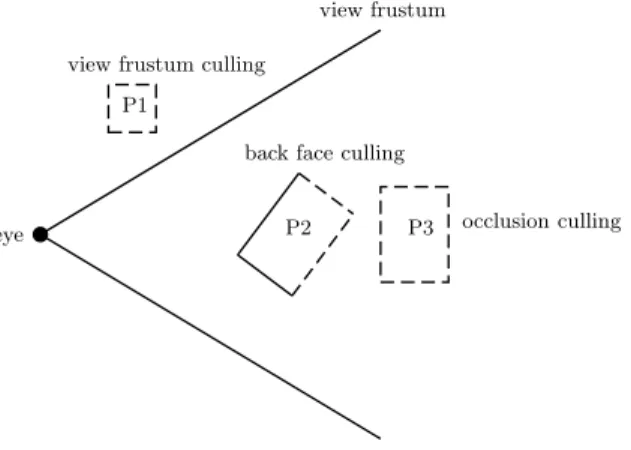
field-of-view, back face culling removes surfaces facing away from the viewer for closed convex opaque objects. Occlusion culling removes objects occluded by objects closer to the viewer, see Figure 1 for the different culling techniques.

The simplest of the three methods to implement are the view frustum- and back face culling. View frustum culling is traditionally implemented using hi-erarchies of bounding volumes or a spatial data structure such as kd-tree or

(5)

eye

view frustum

back face culling

occlusion culling view frustum culling

P1

P2 P3

Figure 1: Examples of the three culling techniques. P 1 is outside the frustum. The back faces of P 2 are culled as they are facing away. P 3 is obscured from the viewer by P 2.

BSP-tree [11]. The hierarchy is then compared to the frustum and the subtrees of the hierarchy that are outside the frustum may be rejected early. Back face culling may be implemented in hardware, but using solely hardware back face culling has the drawback of all objects being sent to and processed through most of the pipeline before they may be rejected. Back facing polygons are trivial to determine by inspection of the face normal [21]. Thereby it is more common to perform back face culling in software in order to avoid sending unnecessary data through the pipeline. Occlusion culling is more complex to implement as it involves relationship between the objects in the scene. An object obscuring other objects is called occluder and an object being obscured is referred to as an occludee.

1.1.3 Overview of occlusion culling techniques

The different occlusion culling techniques can be classified on following taxon-omy depending on their specific characteristics [5].

Conservative or Approximative Depends on which PVS the algorithm is designed to calculate. Finding the exact visibility set is too time consum-ing and in practice rarely or never used for occlusion cullconsum-ing. Instead, the algorithm tries to find an approximate or conservative set. Conservative algorithms overestimate the PVS and are most common as they guar-antee a correct image whereas the approximate algorithms might falsely cull visible objects. Algorithms such as Hierarchical Occlusion Maps [9] have approximative features depending on how far away in the scene the primitives are, see section 1.2.2.

From-point based or from-region based From-region or viewcell-based al-gorithms perform the culling calculation on a region of space, meaning that as long as the viewpoint is within a region no recomputation of the PVS is needed. In effect the computation is amortized over several frames.

(6)

In contrast, from-point based algorithms performs the calculation for a discrete point and visibility is recomputed each frame.

Precomputed or Online Algorithms relying on precomputation perform part of the visibility computation as a preprocess stage, typically when the scene is loaded. This increases the speed of the visibility determination and is sometimes a prerequisite for the algorithm to expose real-time be-haviour. Most of the from-region based algorithms have a precomputation stage.

Image Space or Object Space Depending on where the actual visibility culling occurs, occlusion culling algorithms may be broadly categorized into image-space and object-image-space algorithms. Image-image-space algorithms operate on discrete pixels in the image with a finite resolution, they tend to be more robust then object-space algorithms which suffer from numerical preci-sion problems. Image-space approaches are often simpler to implement. Examples of algorithms are Hierarchical Z-buffer [12] and Hierarchical

Occlusion Maps [9].

1.2 Classical occlusion culling algorithms

Much research has been done in the area and occlusion culling is a vital part of almost all interactive graphic applications as a mean to increase performance. In the next section a couple of classical algorithms are presented of which some are outdated but their concepts are very much valid today.

1.2.1 Hierarchical Z-buffer

Hierarchical Z-buffer (HZB) as a software based occlusion culling technique is today outdated, but its concept is still very valid and forms the basis on which many algorithms are built [12]. Today, hierarchical Z-buffer units are implemented in hardware in addition to the z-buffer, known as Z-culling [1].

The outline of the algorithm is as follows; first an octree containing all the objects of the scene is created. The octree is traversed and if the cube is not outside the view frustum the face of the cube is scan converted and compared to the z-buffer. If the face is hidden the objects in the whole cube are hidden and may therefore be discarded. Otherwise traversal continues down the octree. When a leaf cube node is reached and its face is found to be visible the geometry is sent to the rendering pipeline. The scan conversion is expensive for large faces, typically cubes near the root of the octree. Therefore an image-space Z-pyramid is used, where the finest level of the pyramid is the original z-buffer. The values in the z-buffer are then combined 4 by 4 to produce coarser levels. To use the z-pyramid for visibility test the finest level sample which corresponds to the bounding box of the octree cube is chosen.

As the scene being partitioned into an octree the algorithm is exploiting object-space coherence and image-space coherence by the use of the Z-pyramid. Apart from this also temporal coherence is utilized by the maintenance of a recently visible list. The actual culling is done on the z-pyramid, the algorithm should therefore be considered as an image-space algorithm. The problem with this algorithm is the overhead of scan conversion of the faces and the creation

(7)

of the z-pyramid [12]. Furthermore, dynamic scenes are troublesome because of the need to maintain the octree.

1.2.2 Hierarchical Occlusion Maps

Hierarchical Occlusion Maps or HOM [9] decompose the occlusion culling prob-lem into two tests, a 2D overlap test and a depth test. The overlap test decides whether a primitive in image-space is covered by an occluder. The depth test determines if the primitive is behind the occluder. The overlap test is done using a hierarchy of occlusion maps, created by rendering the occluders to the framebuffer. The rendered image form the finest level of the map and coarser levels are produced by averaging squares of 2x2 pixels, resulting in half the res-olution at each level. Figure 2 depicts a HOM, the outlined square in the image correspond to the same area in all pictures and give an example of the decrease in resolution for each coarser level.

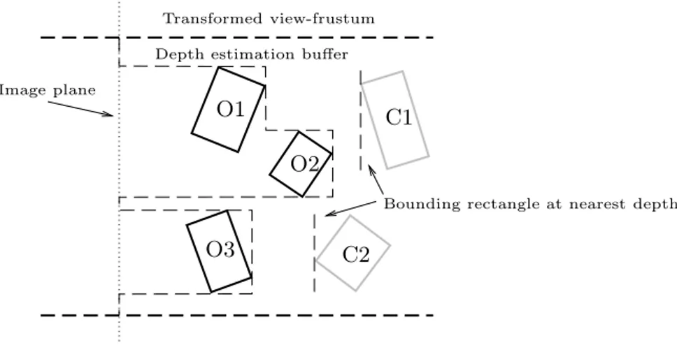
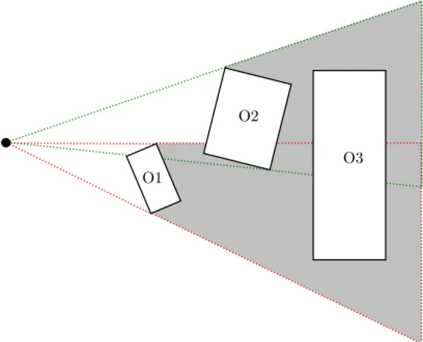
Figure 2: Pyramid with occlusion maps. Reproduced with permission [9]. During overlap test the eight corners of the bounding box of the potential occludees are projected to screen-space. The level in the map where one pixel covers the same space as the bounding box is chosen as start map. If the box overlaps pixels which are not opaque the box cannot be culled. If on the other hand the box is covered by opaque pixels the box might be covered if the box is behind the pixels. This is tested in the depth test phase using a depth estimation buffer. The depth buffer is partitioned on pixel granularity and the

(8)

vertex farthest away from the camera of the bounding box of the occluders is written to the buffer. This buffer is compared to the vertices of the bounding box of the occludees as depicted in Figure 3. Occludee C1 and C2 is behind the occluders at the furthest depth of the occluders and can therefore be culled. The resolution of the depth estimation buffer does not need to match the screen resolution. It’s feasible to have lower resolution as accuracy is already limited by the use of bounding boxes.

O1

O3

O2

C2

C1

Transformed view-frustum Image plane

Depth estimation buffer

Bounding rectangle at nearest depth

Figure 3: Depth resolving with depth estimation buffer.

A nice feature of this algorithm due to the use of occlusion maps for overlap tests is that it exploits occluder fusion. The coverage area of all the occluders is considered. Furthermore it can utilize hardware features such as mip-mapping when the occlusion maps are created [13].

1.2.3 Portal Culling

Portal culling algorithms are a category of culling algorithms developed for ar-chitectural scenes where walls often act as large occluders but are intersected with doors and windows [1]. The algorithm uses view frustum created around the doors to determine the visibility of objects seen trough the doors and win-dows. Usually a preprocess stage is incorporated where the scene is divided into cells corresponding to rooms and hallways. The doors and windows connecting the rooms are referred to as portals, hence the name portal culling.

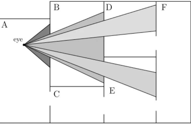
Refer to Figure 4 for a description of portal culling. The eye is positioned in cell A and the field-of-view is depicted in dark grey. Using view frustum culling it is determined that the portal connecting cell A and C is not visible as it is not intersecting the frustum, therefore cell C is omitted from rendering. The portal connecting cell A and B is intersecting the frustum therefore a diminished frustum (light grey) is constructed around the portal and the geometry in cell B is rendered (culled against the frustum). The portals connecting cell B and D and cell B and E are intersecting the frustum and new frustums are created for

(9)

A

B D F

C E

eye

Figure 4: Portal culling.

these portals and the geometry is rendered in both cell D and E. The portals between cell D and F and between E and F are not intersecting either frustum therefore cell F is omitted.

Different techniques may be used to find the portals, one approach is to project each portal to screen-space and finding the axis aligned bounding box around the portal from which the frustum is created [17].

1.2.4 Shadow Volumes

The concept of shadow volumes were first introduced by Crow [8] and are in many senses analogue with the cameras view frustum. A shadow volume de-scribes the region being shadowed by objects obscuring the light emitting from a point light. This could be used for occlusion culling, an example of this were presented by Hudson [14]. The algorithm is point-based with a preprocess step where the scene is spatially subdivided into regions. Each region store a list of potential good occluders selected on their solid angle [14] in relation to all the viewpoints in the region. These occluders are then used in run-time by considering the list of potential occluders lying in the region where the current viewpoint is. For each occluder, a shadow frusta is constructed with its apex at the viewpoint. The near plane of the frustum is defined as a plane passing through the farthest point of the occluder. The actual culling is done for each frustum against the scene described as a bounding volume hierarchy. This algo-rithm differs from HOM and HZB as it is based on the occlusion of primitives in object-space.

2 Occluder fusion

Occludees which are not totally obscured by the occluders when tested discretely may be obscured when two or more occluders are grouped together into a bigger occluder. The method to aggregate occluders is referred to as occluder fusion. Figure 5 depicts fusion of two occluder shadows. Taking advantage of some means of occluder fusion could increase the effectiveness of a occlusion culling algorithm.

(10)

O2

O1

O3

Figure 5: Fusion of two occluders. The shadow frusta for O1 and O2 occludes O3.

2.1 Related work

Several proposed algorithms exist for occluder fusion. Most of them are view-cell based algorithms with a preprocess stage as an integral part to give the algorithms interactive capabilities.

2.1.1 Virtual Occluders: An efficient intermediate PVS representa-tion

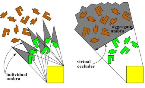
The proposed algorithm performs aggregation of the umbrae of several occlud-ers [15]. The notion of virtual occludocclud-ers are introduced as being the aggregated umbrae of several occluders viewed from any point within a given viewcell. Hence, a virtual occluder is hidden from any viewing point within the viewcell, see Figure 6. The scene is partitioned into a uniform grid of viewcells and in a preprocess stage a set of potential virtual occluders are calculated. During the online stage the P V S is constructed once for each cell using the subset of virtual occluders. The virtual occluders for each viewcell are constructed by selecting a seed object based on the solid angle criteria [14] defined from the centre of the viewcell. Having the seed object, lines are drawn from the viewcells extents to the seed object extents. The lines are moved to include the objects which intersect the lines.

This way a dense set of virtual occluders are created for each viewcell, how-ever as reported just a subset of these are needed for sufficient culling. Therefore a heuristic based on the occluders areas are proposed to decimate the set [15]. The described method is simple enough in 2D, but extending it to 3D increase the complexity considerable. Therefore it is proposed not to use full 3D visibility culling but instead use 2.5D. This is done by discretising the scene in numerous heights and considering each height as a 2D case by limiting the occluders to rectangular occluders.

(11)

(a) Individual umbra for each occluder. (b) Aggregation of umbra into a virtual oc-cluder invisible from the view-cell.

Figure 6: The union of the individual umbra compared to the aggregated umbra. Reproduced with permission [15]

2.1.2 Conservative Volumetric Visibility with Occluder Fusion Proposed is a conservative viewcell based method using the opaque interior of objects as occluders [19]. It exploits the fact that occluders may be extended into empty space as long as that empty space is hidden.

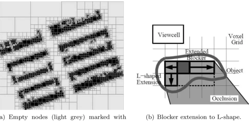
The scene is represented as a quad-tree in 2D and as an octree in 3D. The interior of the objects in the scene are distinguished from the exterior by mark-ing every node in the tree containmark-ing an object face as a boundary node. A flood-fill algorithm is then used to mark the empty nodes, (light grey in 7(a)). The remaining nodes are thereby the opaque nodes (black in Figure 7(a)) and represent potential occluders.

The next step is to find and extend the occluders (opaque nodes in 7(a)). The tree is traversed until an occluder is found which is then extended laterally along the coordinate-axis until a non-opaque node is encountered. If more than one side is visible from the viewcell it is extended along that side to an L-shape (7(b)). The shape composed of voxels in the grid is referred to as a blocker.

The next step is to extend the blocker into hidden space. All space behind the

blocker is hidden and might be treated as opaque therefore blockers intersecting

the umbra are fused together.

Lastly a shaft is constructed using the supporting plane between the view-cell and the blocker. The supporting plane is composed by an edge from the

blocker object and a vertex from the extent of the viewcell. As for the algorithm

(12)

(a) Empty nodes (light grey) marked with flood-fill.

(b) Blocker extension to L-shape.

Figure 7: Figures depicting the flood-fill of the octree nodes and the blocker. 2.1.3 Visibility Preprocessing with Occluder Fusion for Urban

Walk-throughs

The algorithm presented is a conservative occlusion culling algorithm based on from-cell visibility [22]. The visibility from a cell is calculated offline by sampling visibility from the point boundary of the cell.

Figure 8: Occluder shrinking to the left and fused umbra from 5 sample points to the right. Image reproduced with permission [22].

Figure 8 depicts the idea of the algorithm; every occluder is shrunken by epsilon. A number of sample points are chosen on the view cell and the occlusion is calculated on the occluders from these sample points. The sample points are distributed over the viewcell with a gap no greater then ǫ. In that way an object classified as occluded will still be occluded if the viewpoint is moved no more then ǫ distance from its original point. Occluder fusion can be preformed using two different approaches.

• If the PVS is known for each viewpoint, the PVS for the cell is simply the union of the P V S for the points.

• If the umbra is stored explicitly at the point visibility algorithm, the joint umbra may be calculated by intersecting the point umbrae.

(13)

In order to reduce complexity, the environment tested is a city-like scene (2.5D). Because of the 2.5D property of the occluders an object found visible from one point will also be visible from all points above the sample points. Therefore, the sample points need only to be placed on the top edge of the viewcell. The number of point samples needed in 3D would be large, and is not considered in the report.

2.1.4 Conservative Visibility Preprocessing using Extended Projec-tions

Proposed is another cell-based occlusion culling algorithm [10]. The P V S is constructed in a preprocess step. The notion of extended projection is intro-duced which permits conservative occlusion culling in relation to all viewpoints within a cell. Furthermore the algorithm also exploits occluder fusion. The algorithm’s unique approach is that via the extended projection generalize the idea of occlusion maps to volumetric viewing cells.

The scene is divided into cells and for each cell a PVS is computed. Ex-tended projection is used for the calculation which underestimates projection of occluders and overestimates the projection of the occludees.

Consider Figure 9, the occluders A and B are projected onto the projection plane from the extents of the viewcell. The intersections of these projections (dark and light grey on the projection plane) are the resulting occluder. The occludee is constructed by projection of the union (green) on the projection plane. Hence, the algorithm overestimates the occludee and underestimates the occluder. For depth comparison the z-values of the projected occluder furthest away from the camera is used. One drawback is that occluder efficiency might be decreased as the occluders are underestimated and the occludee overestimated.

Figure 9: Occluder fusion by extended projection. Figure reproduced with permission [10].

(14)

3 Thesis

The objective for this thesis is to extend an existing occlusion culling system to take advantage of occluder fusion. The existing system named Brute Force Box

Culling (BFBC) has been developed by Avalanche studios.

3.1 Brute force box culling

BFBC is designed to handle large flat datasets of potential occludees (AABB) and occluders (OBB). The occluder OBBs are constructed and placed in the scene by hand. Both the AABBs and OBBs must be in-memory even for very large scenes. BFBC is designed using the concept of Data Oriented Design, see appendix A. BFBC is an object-space culling system using frustum created around occluder OBBs for culling of AABBs

The outline of the algorithm is as follows: Each frame a maximum of 256 occluder candidates are chosen, in order to be considered the occluders need to be within a certain distance from the camera. The candidate set is sorted on the distance from the camera and the set is iterated. For each OBB candidate its silhouette is extracted and the silhouette is used to construct frustum-planes around the silhouette. As the occluders are OBBs, the silhouette will have a maximum of 6 sides resulting in 6 frustum planes. The near plane of the frustum is chosen so the objects within the frusta are guaranteed to be hidden. This is guaranteed if the plane is positioned at the vertex point furthest away from the camera with its normal facing the camera. To increase effectiveness more then one plane is used for near plane allowing for a combination of slant planes. The code is SIMD optimized, therefore a multiple of 4 planes are used for each frustum, resulting in at least 2 planes available as near planes if the number of side planes are 6. In current implementation a maximum of 16 frustums are used for occlusion culling of which one is the view frustum, therefore as soon as 15 occluder frustums are created the iteration stops.

The system is designed to handle scenes where the occluders are relatively few and large. For example, big outdoor scenes with large buildings having no or few holes. Potentially good occluders are typically large solid concrete buildings, silos and so forth which easily can host large inscribed occluder OBBs. However, in indoor scenes, with doors and windows it is harder for BFBC to perform well. Main reason is that few large occluders may be placed in an indoor scene beforehand as these scenes typically have doors and windows. In order to handle these scenes better a solution is to have several small OBB occluders inside walls and roofs and let BFBC fuse these occluders.

In order to implement occluder fusion in the context of BFBC there are some preliminaries that need to be considered.

• Occluder fusion must be done on the CPU, without help of the GPU. BFBC is destined to run solely on the CPU therefore hardware occlusion queries cannot be used.

• Must be online. The occluders should be calculated each frame. As mem-ory is restricted, the only data that can be assumed to be in-memmem-ory each frame is the OBB and AABB data. It is not an option to have any precalculation done offline and stored in-memory.

(15)

• Integration with BFBC. The occluder fusion system should be used in conjunction with existing system.

3.2 Occluder fusion in BFBC

None of the methods described in section 2.1 are feasible in the context of BFBC for a number of reasons. Virtual Occluders: An efficient intermediate

PVS representation (2.1.1) heavily relies on an offline stage to compute potential

occluders from a given viewcell. The P V S is then constructed for the viewcell in an online stage amortizing the P V S over all the frames of the viewcell. Having a preprocess stage for computation of potential occluders could not be used as this will increase memory demand. A possibility would be to degrade the algorithm to use point view and recalculate the potential occluders every frame. In such a case the amortizing of the calculation over several frames is lost and the question comes down to if the virtual occluders can effectively be constructed in every frame. The virtual occluder construction is easy enough in 2D but as an implementation for 3D is needed this would significantly increase the complexity. In such a case it is suggested to discretise the scene in numerous heights resulting in a 2.5D problem [15]. However this implies that the seed occluders must be rectangular in shape at each discretised height. As the indata is OBB this would result in finding an AABB inscribed inside the OBB which is a complex task in 3D and will in the same time diminish the usable occluder area.

Generally viewcell based algorithms are not applicable as they all rely on amortizing the cost for occluder fusion over several frames. Meaning calculated data must be saved over frames and thereby increasing the memory demand. Furthermore, almost all proposed algorithms rely on complex data structures as a prerequisite to use viewcell based approaches this further disqualifies them.

Conservative Volumetric Visibility with Occluder Fusion (2.1.2) depends on

complex datastructures such as quad-tree and octrees which thereby disqualifies this algorithm to be used in conjunction with BFBC. Furthermore the algorithm is viewcell based.

Visibility Preprocessing with Occluder Fusion for Urban Walkthroughs (2.1.3)

is yet another viewcell based algorithm which inherently miss the sought goal of aggregation of oriented boxes each frame.

Also Conservative Visibility Preprocessing using Extended Projections (2.1.4) is a viewcell based approach which use the idea of occlusion maps. As viewcell based approaches is not applicable this algorithm does not bring anything that might be useful other than a traditional occlusion map.

Looking at an approach were a HOM or HZB is used could be beneficial as many of their features are favourable, not least the inherent occluder fusion. However, these algorithms rely on the z-buffer and rasterization of the scene which traditionally is done on the GPU. Therefore an implementation of the rasterization pipeline has to be done in software. One approach would be to use BFBC for view-frustum culling only and complement the system with an image-space approach for the occlusion culling within the view frustum. Such an approach is taken by DICE in their Frostbite engine, where a low resolution rasterization of the occluders is done to an occlusion map [7]. The rasterization step is reported to add overhead, a method avoiding this extra step is therefore sought. The notion is to still conduct all occlusion culling in object space with existing system and thereby avoid much redesign of BFBC. In order to fuse

(16)

oc-cluders without rasterization the option is to either fuse the silhouettes produced by BFBC or to fuse OBBs and extract the silhouette afterwards. Aggregate ob-jects, albeit simple objects such as OBB in objects-space are cumbersome and no real usable methods were found in this case. Therefore, reducing the problem from 3D to 2D seams like an attractive approach. However conversion back to 3D must be possible to conduct the actual culling in 3D in order to conform to the existing system.

3.2.1 Method 1: Axis-Aligned fusion

The algorithm proposed performs fusion of axis-aligned rectangles (silhouettes). The algorithm conforms to the requirements of being online and is intended to run its calculation each frame. The algorithm do not rely on the GPU, it is implemented solely on the CPU and is integratable with BFBC. As the algorithm uses axis-parallel rectangles it will probably not handle scenes where the silhouettes have slant edges very well. This is dealt with by extending the algorithm to handle n-gons, see section 3.2.4.

3.2.2 Algorithm overview

The algorithm consists of a number of steps outlined below: • Construction of silhouettes for each OBB.

• Transformation of silhouettes to Normalized Device Coordinates (NDC) and conversion to fixed point integer coordinates.

• Creation of axis-aligned rectangles inscribed in the silhouettes. • Fusion of the axis-aligned silhouettes.

• Conversion of the fused silhouettes back to world-space and construction of occluder frustums.

Indata is a collection of silhouettes constructed from the occluder OBBs. A maximum of 256 occluders nearest to the camera are chosen as candidates. All silhouettes are guaranteed to have four or maximum six sides and are given in object-space. The silhouettes are transformed to clip-coordinates by transfor-mation with the view and perspective matrix and to Normalized Device

Coor-dinates (NDC) by division with w. To avoid precision problems the coorCoor-dinates

are then converted from float to fixed point integer coordinates. Some points of the silhouette edges might lie outside the unitcube. Therefore the edges must be clipped to the unitcube otherwise values outside would wrap around when converted to fixed point integer coordinates.

Next an inscribed axis-aligned rectangle is calculated for each silhouette. Figure 10 depicts the data structure for an axis aligned silhouette. Along with the minimum and maximum integer coordinates, the z-value of the point furthest away in the original OBB is stored to be used when the distances between silhouettes should be calculated at a later stage. Also, the index corresponding to the OBB from where the silhouette was extracted is stored for later use.

(17)

axis aligned silhouette {

point min, max; float distance; int obb_index[4]; }

Figure 10: Datastructure for an axis-aligned silhouette.

3.2.3 Silhouette fusion

The collection of axis-aligned silhouettes is in the next stage fused. The silhou-ettes are sorted on distance from the camera, with the nearest silhouette first. Every possible intersection among the silhouettes is calculated. In order to get a reasonable good fusion a graph [20] is constructed describing the topology of the intersections. The edges of the graph represent overlaps and the nodes the actual silhouettes.

The graph is constructed by iterating the silhouettes starting with the sil-houette nearest to the camera. Each intersecting silsil-houette is considered and if the distance to the first silhouette is not above a certain threshold, the silhou-ette is added as a node in the graph. This procedure is repeated until no more silhouettes within reach can be added. All the silhouettes which are now part of the graph are removed from the list of silhouettes and the next silhouette of the remaining silhouettes are fed to the graph creation algorithm. The graph will typically consists of several subgraphs as only overlapping silhouettes within a specified maximum distance between the nearest and furthest silhouette are considered. S1 S2 S3 S4 S5 S6

(a) Overlapping silhouettes. S1–S4 and S_{5–S6 will reside in each subgraph.}

S2 S3

S4

S1

S5 S6

(b) Graph containing two sub-graphs.

Figure 11: Silhouettes with corresponding graph

As can be seen in Figure 11 the silhouettes S4 and S5 are overlapping but the distance from the first considered S1 to S5 is too far, therefore S4 have no edge to S5. Instead S5 and S6 will reside in their own subgraph. In the next stage the subgraphs are used to construct fused silhouettes.

The algorithm for the fusion is shown in Figure 12. FuseSilhouetteInGraph takes a graph G consisting of several subgraphs as input. The subgraphs are

(18)

iterated (Line 2) and for each subgraph the node n with the silhouette having the largest area is selected as startnode (Line 3). The silhouettes in the subgraph Gi are fused in the method Aggregate (Line 4) taking the startnode n and the current subgraph Gi as parameters. The returned aggregated silhouette is assigned to the output collection Sj.

FuseSilhouettesInGraph input: G = {G0, G1, . . . , Gn} output: S = {S0, S1, . . . , Gn} 1. j = 0 2. for each Gi∈ G 3. n← GetLargestNode(Gi) 4. Sj← Aggregate(Gi, n) 5. j = j + 1

Figure 12: Pseudocode for fusion of silhouettes in the graph.

The Aggregate method is shown in Figure 13. Taking a subgraph g and the node n with the largest area as input. First the node n is used to determine the best silhouette to fuse with (Line 1). FindBestIntersection takes the current node n as input and returns the edge e of the node having the best overlap with node n. Furthermore it returns the axis a, which should be the start axis for the expansion in FuseShilouettes. FuseSilhouettes takes the node n and the best overlap edge e along with the advised axis a as parameters and returns the fused silhouette s (Line 2). If this aggregation is found to be less in area than the silhouette in the startnode n (Line 3), this fusion is considered a bad alternative and the node associated with the edge e is removed from the graph (Line 4). If however, the aggregation is bigger, a new node is constructed for the aggregated silhouette s and added to the graph (Line 6). The nodes for the silhouette that were fused and their edges are in the same operation removed in

AddNodeAndUpdateGraph (Line 6). The newly created node is assigned to n. Aggregate is called recursively for all edges in the node (Line 8).

FindBestIntersection and FuseSilhouettes need some further explanation.

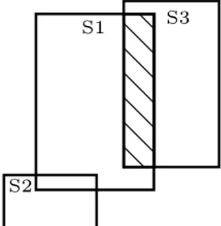
The principle for FindBestIntersection is depicted in Figure 14. The overlap of S3 on S1 on the y-axis is of a larger degree than the overlap of S2 on S1 on the x-axis, therefore the edge between S1 and S3 is considered to be the best intersection. As the best overlap were on the y-axis, it is best to start the fusion along the x-axis, therefore the x-axis is advised to be the start axis for fusion to FuseSilhouettes (Line 2), Figure 13.

The principle for FuseSilhouettes is shown in Figure 15. Taking the node n and the best overlap edge e along with the advised axis a as parameters. The algorithm starts by placing a small axis-aligned rectangle r in the centre of the intersection, Figure 15(a). As expansion should be started on the x-axis the minimum and maximum value of r is set to the minimum and maximum value of S1 and S3, depicted as red dots in Figure 15(a). The minimum and maximum y-value of r is set to the minimum and maximum of the intersection, resulting in a fused silhouette depicted in Figure 15(b).

(19)

Aggregate input: g, n output: s

1. a, e ← FindBestIntersection(n) 2. s ← FuseSilhouettes(e, n, a) 3. if area(s) < area(n) then 4 RemoveNode_{(g, e)} 5. else

6. n← AddNodeAndUpdateGraph(g, s) 7. if edges(n) > 0 then

8. Aggregate_{(n, g)}

Figure 13: Pseudocode the aggreagtion algorithm.

S1

S2

S3

Figure 14: Example of which intersection is considered the best overlapp for fusion.

As the algorithm starts the aggregation with the largest silhouette from each subgraph and selects the intersection with the biggest degree of overlap. The following heuristic is enforced:

• Try to aggregate the largest silhouettes with each other and avoid aggre-gation of a big and a small silhouette.

• Primarily aggregate silhouettes having the largest degree of intersection on either of the silhouettes sides.

The occlusion culling should be performed with frustum planes in object-space therefore the axis-aligned fused silhouettes are converted back from fixed-point integer coordinates to world-space. To get the z-value for the min/max points a ray cast is preformed from the camera position to the corner points of the silhouette. The z-value is set to the value where the ray intersects the front-facing faces of the OBBs. Which corner points corresponding to which OBB were saved in axis aligned silhouette, Figure 10. Having the coordinates for the extent of the silhouettes, the frustum planes may now be constructed and fed to BFBC.

(20)

S1 S3

(a) Rectangle expanded on x-axis first.

S1 S3

(b) Expanded to itersections on y-axis.

Figure 15: Aggreagtion of two silhouettes. 3.2.4 Method 2: n-gon fusion

The downside of Method 1: Axis-Aligned fusion algorithm is the potential to loose occluder power due to the use of axis-aligned silhouettes. Therefore a progression of the algorithm is proposed which handle fusion of n-gons. The core of the algorithm builds upon the work by Cohen [6] where inscribed polygons are found within a concave shape. The first steps of the algorithm are similar to

Method 1: Axis-Aligned fusion. Silhouettes are extracted from occluder OBBs

and converted to clipped Normalized Device Coordinates(N DC) which are then converted to integer coordinates. Then the process differs from the former, instead of a graph creation, concave silhouettes are constructed of the union of overlapping silhouettes and convex inscribed polygons are found within the concave silhouette. The notion of Cover is used as being large inscribed convex polygons within a concave silhouette. The algorithm is not optimal in the sense that it finds the biggest possible inner cover as such an operation have been reported to have a complexity of O(n9_{log n) where n is the number of vertices} in the polygon [4].

The input data is OBBs from where silhouettes are constructed and trans-formed to fixed-point clipped Normalized Device Coordinates. Next the outline of the algorithm is as follows:

• Create unions of the overlapping silhouettes. • Remove redundant points.

• Create an Arrangement of the silhouettes in the union. • Decompose the Arrangement into a number of convex faces.

• Find convex Covers by combining the faces of the Arrangement to convex polygons.

• Choose the largest polygon of each Cover as the occluder silhouette. In the first stage the silhouette unions are created with the greedy algorithm shown in the pseudocode in Figure 16. In most cases the union of the silhouettes will be concave in shape therefore the created unions are referred to as concave

(21)

CreateConcaveSilhouette input: S = {S0, S1, . . . , Sn} output: F = {F0, F1, . . . , Fm} 1. j = 0

2. do while S not empty 3. s← PopFront(S) 4. d← Distance(s) 5. for each Si∈ S

6. if Distance(Si) − d < max distance then

7. u← CreateUnion(s, Si)

8. if not ContainHole(u) then

9. s← u

10. S← RemoveSilhouette(Si)

11. Fj← s 12. j = j + 1

Figure 16: Pseudocode for concave silhouette creation.

silhouettes. Input to the algorithm is a collection of silhouettes S ordered by the distance to the camera. The first silhouette is popped from the silhouette collection (Line 3) and assigned to s. The distance from the camera to the silhouette is stored in d (Line 4). The rest of the silhouettes in the collection are iterated (Line 5-10). If a silhouette Si is found to be within max distance from the first (Line 6), a union is created of the silhouettes s and Siand assigned to u (Line 7). For a union to occur the silhouettes must be overlapping and the union must not result in any holes (Line 8).

The silhouette Si which was fused with s is removed from the silhouette collection and not considered again (Line 10). Then the rest of the list S is iterated, the resulting combined silhouette s is assigned to the collection of concave silhouettes F (Line 11). If there are any remaining silhouettes in S the process is repeated (Line 2).

Each concave silhouette may have several collinear points. It is desirable to have no more vertex points than needed as more points increase the complexity of the faces created in the next stage. Therefore each silhouette is iterated and if three or more vertices points are found to be on the same line the redundant points are removed.

3.2.5 Inscribedn-gons

In the next stage, inscribed convex n-gons are found within the concave sil-houette, for an inscribed polygon the notion of Cover is used as the objective is to find convex polygons that cover as much of the concave outer silhouette as possible. A concave polygon may be partitioned into a number of convex polygons by extension of the lines at each reflex point. This is due to the fact that a line which coincides with the edges at a reflex point is guaranteed to cut the reflex angle into two convex angles. Figure 17 displays the cutting lines of

(22)

a concave polygon. The red dot marks the reflex point of the polygon and by cutting the polygon along the two lines that coincide with the reflex point, the concave polygon is decomposed into three convex polygons.

Figure 17: Reflex point in a concave polygon.

The process of finding the Cover inside a polygon is depicted in the pseu-docode in Figure 18. As input the collection of concave polygons F is given. The collection is iterated (Line 1) and for each polygon an Arrangement [18] L induced by the polygon Fi is created (Line 2). An Arrangement consists of vertices, edges and faces and simplifies the handling of the convex faces within the polygon.

Having the Arrangement the reflex points are found and cutting lines at the reflex points are used to decompose the Arrangement into convex polygons (Line 3). With the Arrangement consisting solely of convex polygons an inner convex Cover is found in the next step (Line 4). Of all the found polygons in L the one with the largest area is added to the resulting list of silhouettes Pi (Line 5). CreateInscribedPolygon input: F = {F0, F1, . . . , Fn} output: P = {P0, P1, . . . , Pn} 1. for each Fi∈ F 2. L← CreateArrangement(Fi) 3. L← DecomposeToConvexPolygons(L) 4. c← CreateCover(L) 5. Pi← GetLargetsPolygonInCover(c)

Figure 18: Pseudocode for creation and selection of large inscribed polygons. The process of finding convex inner polygons (Covers) of a concave shape is depicted in Figure 19. Consider the depicted concave shape decomposed into an

Arrangement of convex polygons with faces numbered from 1 to 10. First the

polygon with the largest area is added to the Cover, face number 4 in Figure 19(a). Next, the remaining faces are iterated on descending area and each face is combined into a convex hull with each of the polygon in the Cover. As there is only one polygon in the Cover, this polygon is combined with face number 9. The convex hull around face 4 and face 9 is within the Arrangement therefore

(23)

1 2 3 4 5 6 7 8 9 10 (a) 1 2 3 4 5 6 7 8 9 10 (b) 1 2 3 4 5 6 7 8 9 10 (c) 1 2 3 4 5 6 7 8 9 10 (d) 1 2 3 4 5 6 7 8 9 10 (e) 1 2 3 4 5 6 7 8 9 10 (f)

Figure 19: Create Cover process. The greedy process resulting in three polygons in the cover, marked with green, red and grey.

the Cover is updated to contain the convex hull of 4 and 9, Figure 19(b). The next face considered, number 2, cannot be added to existing Cover (4 and 9) as the resulting convex hull would be outside of the Arrangement. Therefore face number 2 is added as a new polygon to the Cover, Figure 19(c). Next, face number 1 is considered, it cannot be added to the grey polygon as the resulting convex hull would be outside the Arrangement, but it can be added to the green polygon, Figure 19(d). The process continues considering the faces in ascending order and tries to combine the faces with each of the polygon in the cover. In Figure 19(e), face number 10 has been added to the grey polygon and face number 6 is added as a new polygon to the Cover. The resulting Cover is depicted in Figure 19(f). Face number 5 is added to the grey polygon, face number 3 and 8 is added to the green polygon and face number 5 and 7 is added to the red polygon.

The pseudocode for the described process is depicted in CreateCover, Figure 20. As input the Arrangement L is given and for this Arrangement a Cover P consisting of several polygons is returned. First the faces are sorted on area in descending order (Line 1). The largest face f is assigned to be the first polygon in the Cover P0(Line 3). The faces are then combined with the polygons in the

Cover. This is done by iterating over the list of faces (Line 4) and combining

the faces with the largest polygons in the Cover. Broken down, for each face the polygons in the Cover P are sorted on area in descending order (Line 5). For each polygon Pj in the Cover P a convex hull is created of the face fk and the polygon Pj(Line 8). If the created hull h is found to be inside the Arrangement L, the current polygon Pj of the Cover is updated (Line 9-11). If however the face fk could not be combined with any polygon in the Cover, the face fk is added as a new polygon in the Cover (Line 12-14). The simple heuristic used for this process is to begin with the largest face and then try to combine each

(24)

face with the largest polygon in the Cover first. As reported this heuristic is found to generate the Cover with the largest cover ratio [6].

CreateCover input: L output: P = {P0, P1, . . . , Pn} 1. f ← GetSortedFaceList(L) 2. i = 0 3. Pi= f0 4. for k = 1 to NoOfFaces(f ) 5. SortPolygonsOnArea_{(P )} 6. cover updated=false 7. for each Pj ∈ P 8. h← CreateConvexHull(Pj, fk) 9. if IsInside(h, L) then 10. cover updated=true 11. Pj← h

12. if not cover updated then

13. i= i + 1

14. Pi← fk

Figure 20: Pseudocode for cover creation.

As mentioned, of all the created polygons in the Cover, the one with the largest area is selected as occluder silhouette from the Cover, Figure 18 (Line 5). Having these silhouettes the 15 nearest to the camera are selected as occluder silhouettes. In current implementation a frustum can have no more then 15 planes (15 side planes + 1 for the near plane), therefore silhouettes having more then 15 sides are disqualified.

The silhouette points are converted back to floating point values in world space. In order to get the z-value for the points the same method is used as for Method 1: Axis-Aligned fusion; A raycast is performed from the camera through the silhouettes points. The z-value is then set to the point were the ray intersects the OBBs face.

The frustum’s near plane is constructed by taking the near plane from the camera frustum and move it to the furthest point of the edges in relation to the camera. The limit of 15 side planes + 1 far plane is due to conform to SIMD optimized culling utilized by BFBC.

3.3 Results

The developed algorithms were tested in two different environments. The first consists of a number of axis aligned boxes as potential occludees with random heights distributed over a plane in the scene. The placements of the boxes on the plane were also randomized to some extent to avoid long rows of boxes behind each other. For each box a hidden OBB occluder were created.

The second test environment Suburban depicts houses and fences in a sub-urban in order to simulate a more realistic scene. In each house a number of

(25)

occluders were placed.

For each environment 3 different test scenes were used. Metrics data re-ported for each scene is the number of occluders used, how many objects that were culled, presented as the actual number of objects and as a percentage in relation to the number of total objects in the scene. As comparison the BFBC algorithm is presented along with the culling efficiency when only the view frus-tum culling is used. For Method 1: Axis-Aligned fusion it is also presented metrics for when this algorithm is combined with BFBC. In the combination 7 of the allowed 15 occluders where the biggest calculated fused occluders and the other 8 were discrete occluders. If 7 fused occluders could not be found more discrete occluders were used until the limit of 15 were reached.

Three pictures are displayed for each scene, the first is a rendering of the scene from the camera, the second displays the concave silhouettes outlined in yellow and the last picture displays the fused silhouettes in green. All the pictures are the silhouettes produced by Method 2: n-gon fusion.

3.3.1 Boxes

Below are metrics data from 3 box scenes, total number of object in each scene is 256.

(a) Scene as seen from the camera. (b) Silhouettes outlined in yellow.

(c) Fused silhouettes in green.

Figure 21: Box scene 1.

Scene 1 A hard scene for any good occluder fusion to occur. The boxes are too aligned so little fusion occurs. Method 2: n-gon fusion does not suffer for

(26)

Method _Occluders _Culled _Efficiency _Fusion+BFBC

Only frustum 65 25.39%

BFBC 15 123 48.05%

Method 1: Axis-Aligned fusion 4 90 35.15% 47.26% Method 2: n-gon fusion 12 122 47.66%

Table 1: Result for box scene 1.

this to the same extent as Method 1: Axis-Aligned fusion. However, the axis-aligned algorithm only performs fusion if a fused silhouette with larger area is found, very few occluders are used and therefore it is unfair to consider just the axis-aligned fusion. A better metric is to look at the axis-aligned fusion algorithm combined with BFBC (Fusion+BFBC ), in such a case the algorithm performs almost as well as BFBC. It is worth noting that fewer occluders, 12 for Method 2: n-gon fusion actually perform almost as well as BFBC with 15 occluders.

(a) Scene as seen from the camera (b) Silhouettes outlined in yellow

(c) Fused silhouettes in green

Figure 22: Box scene 2

Method _Occluders _Culled _Efficiency _Fusion+BFBC

Only frustum 95 37.11%

BFBC 15 149 58.20%

(27)

Scene 2 Very little fusion can occur in this scene as well, the boxes lies to much aligned and therefore both fusion algorithms perform badly. More so for Method 1: Axis-Aligned fusion as the fused silhouettes cannot benefit from edges not being axis-aligned. Still Method 2: n-gon fusion performs almost as well as BFBC but with fewer occluders.

Figure 23: Box scene 3.

Method _Occluders _Culled _Efficiency _Fusion+BFBC Only frustum 103 40.23%

BFBC 15 167 65.23%

Table 3: Result for box scene 3.

Scene 3 This scene is the only scene where a fusion algorithm actually per-forms better than BFBC due to a couple of good fused occluders in the fore-ground.

(28)

Over all the scenes it is clear that neither of the fusion algorithms contribute to the overall occlusion efficiency. Taking into account the time taken to fuse occluders it would certainly not be beneficial. However the scenes with boxes are not likely to occur in a real world application.

3.3.2 Suburban

Below is metrics data for 3 suburban scenes. The total number of objects in each scene was 500. The suburban scenes can be considered to more resemble scenes that an occluder fusion algorithm should handle. Each house consists of many small occluders (more then 15) placed just inside the walls of each house.

Figure 24: Suburban scene 1.

BFBC 15 306 61.20%

Table 4: Result for suburban scene 1.

Scene 1 Each house consists of more then 15 OBBs, therefore all the occluders used in BFBC will be chosen from the red house in the foreground. For Method 2: n-gon fusion we get a greater spread on the occluders as the first house will result

in two occluder frustums being created and the green and orange houses further away will due to the fusion result in good occluders, Figure 24(a). Method 2:

n-gon fusion algorithm performs better than the others. Fusion+BFBC performs

almost as well as BFBC, because it uses the same occluders as BFBC but they are somewhat shrunken as they are axis-aligned rectangles.

(29)

BFBC 15 339 67.80%

Scene 2 Fusion on the red house in the foreground results in good occluder efficiency for Method 2: n-gon fusion. However, looking at the produced fused silhouettes in Figure 25, it is clear that occluder power is lost on the second house in the scene. If more then one silhouette from each Cover were chosen the second house could be contributing with its whole side as an occluder. Method

1: Axis-Aligned fusion performs really badly because the axis aligned rectangles

are found to be really small in comparison.

BFBC 15 341 68.20%

Scene 3 This is an example where Method 2: n-gon fusion performs badly. The reason is the greedy nature of the CreateConcaveSilhouette algorithm which permits silhouettes with holes being filled. Furthermore, for each concave silhou-ette, only one convex silhouette are chosen. In scenes like this with one building

(30)

close to the camera it would be preferable to use more than one silhouette from each Cover.

3.4 Discussion

As measurement shows, the algorithm with best potential is Method 2: n-gon

fusion. Method 1: Axis-Aligned fusion in conjunction with BFBC at best just

produce the same efficiency as BFBC alone, so the extra work for conducting the fusion is not worth the effort. Therefore in the discussion below only the n-gon fusion algorithm is considered.

(31)

3.4.1 Efficiency

There are many parts of the algorithm that can be refined to result in greater occluder efficiency. Scene 3 is a good example were the fusion performs badly and also a good example of where the algorithm need refinements. First of all the algorithm can not fill holes during the construction of the concave silhouette. The silhouette resulting from the roof is as good as it can be as it is limited by the window in the house. But the left silhouette is limited by the left window marked with yellow in Figure 27. This hole can be filled as it is obscured by the farther side of the house. In such a scenario the left occluder could be extended further to the right.

The suburban scene has no occluders in the floors of the houses, if the

CreateConcaveSilhouette is extended to handle holes, it would make sense to

add floor occluders which in many cases would fill holes.

Looking at the CreateCover algorithm, the produced polygons in the Covers could be made bigger by a proposed enlargement step [6]. When all polygons are created in the Cover, iterate over the polygons and try to combine each polygon with the faces adjacent to the polygon are reported to increase the area of the Cover.

There is no check if a selected occluder silhouette is already occluded by an occluder nearer to the camera. As the total occluder frustums are limited to 15+1 frustums, removing already occluded frustum could be beneficial as all the selected frustums in such a case have the chance to do useful work.

In scene 3 it would definitely be beneficial to select many occluders from the house in the foreground. Instead of discretely considering each Cover con-structed, the final selection should consider all the polygons over all Covers and among this set selecting the most beneficial occluders.

The restriction of a maximum of 16 planes for each silhouette (15 for the silhouette and one for the near plane) is assumed to have small impact on the efficiency as measurement has shown that very few silhouettes are disqualified due to this reason. If needed it would be easy to reduce the number of edges of the silhouette as removing a vertex point from a convex polygon always results in a smaller convex polygon.

3.4.2 Complexity

CreateConcaveSilhouette RemovePointsOnLine CreateInscribedPolygon

10.38% 36.16% 49.69%

9.83% 43.66% 43.46%

10.80% 47.17% 38.28%

Table 7: Relative running time for n-gon fusion.

The relative running time for the different stages of Method 2: n-gon fusion algorithm are shown in table 7, the measurement comes from the three suburban scenes. Looking at table 7 it is clear that two stages answer for the bulk of the running time, CreateInscribedPolygon, Figure 18 consumes around 38% to 49% of the running time and RemovePointsOnLine 36% to 47%.

RemovePointsOn-Line and CreateInscribedPolygon constitute together around 85% of the running

time and as CreateConcaveSilhouette is stable around 10% this is 95% of the total running time for the algorithm. The rest 5% cannot be attributed to

(32)

any specific algorithm and is instead start-up code for the algorithm, dynamic list creation of potential occluders, the selection of the biggest polygon in each

Cover, unitcube-clipping etc.

Consider the CretateInscribedPolygon algorithm, CreateCover answer for 93% to 96% of the running time. In the CreateCover algorithm the creation of convex hulls are the most time consuming with 74% to 76% of the running time.

The total running time in seconds for the algorithm was around 1.0 - 1.5 sec-onds for the tested suburban scenes. The convex hull algorithm is implemented as a Quickhull algorithm [18] which has a worst case complexity of O(n2

). Worst case occurs when the points are ordered and the divide and conquer nature of Quickhull results in a maldistribution of the pointset. A trick to avoid worst case is to randomize the points feed to Quickhull. In the n-gon fusion case the fed points are the concatenation of two ordered pointsets, therefore a randomiza-tion could be beneficial. Something that complicates the implementarandomiza-tion of the Quickhull algorithm is that the output vertices needs to be ordered, therefore sorting having O(n2_{) occurs. Both the maldistribution and the sorting problem} might be avoided if another convex hull algorithm is used, such as Grahams algorithm [18], having complexity O(n log n) and the benefit to give the result-ing hull vertices ordered. Even if a better convex hull algorithm is chosen it is still of interest to call the algorithm no more then necessary. How many times convex hull are executed depends on the number of faces in the Arrangement and how many polygons in the Cover that are created. An Arrangement L limited by a bounding polygon P having n vertices and edges are created with at most 2n lines. If we assume that no faces in the Arrangement can be com-bined in the Cover, the convex hull algorithm will be called at mostPni=1i− 1 times where n is the number of faces in the Arrangement. This is however not likely to occur, but it is never the less important to call convex hull no more then needed. This is accomplished by reduction of the number of faces in the

Arrangement by reducing the number of reflex points in the concave silhouette.

The face reduction could be done by iterating over the vertex points in the concave silhouette and forming triangles with the two neighbouring vertices. If the triangle is contained within the silhouette and is small it may be removed. This simplification stage is reported to reduce the reflex points [6]. Apart from this, it is also suggested that the cover is created up to a certain coverage ratio. This reduces the number of resulting polygons in the Cover.

RemovePointsOnLine answer for 36%-47% of the total running time. The

algorithm is executed two times to make sure as many points as possible are removed. A better solution is to modify the algorithm to produce equally good or better result in one execution which will probably save execution time.

Furthermore, the number of concave silhouettes considered altogether might be reduced. For example, in an interior-like environment the fusion of many small occluders near the camera are of essence, therefore there is no need to consider silhouettes far away. For city-like scenes on the other hand, with a vast horizon and typical city-like environment features like tunnels and bridges, fusion of silhouettes further away could be preferable. Therefore a configurable heuristic for silhouette selection remains to be found.

(33)

3.5 Conclusion

It is clear that just to fuse axis-aligned silhouettes does not produce enough occluder efficiency. A solution with n-gon is needed. Especially for interior scenes with lots of small occluders as this give rise to many silhouettes with slant edges. However, the algorithm does not feature interactive running time in current implementation. If that is possible remain to be investigated.

For suburban scene 1 and 2 the efficiency is around 15% better for Method

2: n-gon fusion than for BFBC, but for scene 3 it is almost 10% less effective.

Therefore if we assume that sometimes the fusion will not contribute with better occluder power, the fusion process must be fast so it is not degrading perfor-mance. Therefore it is safe to assume that the fusion process is not allowed to take more than fractions of a millisecond. In current implementation the tested suburban scenes had a running time of around 1-1.5 seconds. This means that the running time has to be improved with a factor of 10k. It should be noted that the implementation feature no optimization. The Standard Template

Li-brary (STL) were used extensively with lots of dynamic memory handling. The

dynamic memory handling could be avoided completely, even if it would render in a slight degradation of the algorithm. Considering the

CreateConcaveSilhou-ette algorithm, the input silhouCreateConcaveSilhou-ette has a upper limit so no memory allocation

on the fly is necessary. When creating new concave silhouettes a upper limit need to be set how many edges each silhouette may contain. The creation could simply stop when the limit is reached. Looking at CreateInscribedPolygon the dynamic memory handling could be avoided as we know that an Arrangement in theory will contains at most n2 _{edges. Where n is the number of lines in} the Arrangement, hence the number of edges in the concave silhouette. With these suggestions it would be interesting to refine the algorithm to avoid dy-namic memory and refine the crucial part of the algorithm as noted in 3.4.2 in order to come to consensus whether this algorithm could be used in a real-time application.

3.6 Future work

There are many areas interesting for future work, as mentioned under discussion. In order to increase the efficiency, the CreateConcaveSilhouettes could be refined to be able to fill holes. The polygons in the cover could be enlarged further by being combined with adjacent edges. To choose more than one polygon from each Cover and also to remove redundant silhouettes so the maximum slot of 15 occluders only contain frustum that actually contribute to the occlusion would probably increase efficiency. To decrease algorithm running time it would be interesting to simplify the concave polygon and to create Cover just to a certain degree and avoid considering to small faces. Also it would be interesting to investigate a system to avoid considering silhouettes to far away from the camera.

Apart from these refinements it remains to be investigated how to best com-bine the discrete occluders created by BFBC and n-gon fusion. The implemen-tation of today using solely fused silhouettes for culling and only silhouettes that were fused are considered. In order to maximize occluder efficiency, both fused and non-fused silhouette should be used for culling. One possibility is of course to let half of the frustums come from the fused and the other half from

(34)

the discrete occluders as were tested for Method 1: Axis-Aligned fusion. This is not ideal as the silhouette might cover the same area of the screen so a heuristic based on the distribution of the silhouettes over the screen are probably better. The maximum distance allowed between the nearest and farthest polygon in the fusion is set to a static value which has proved to be best for the scenes investigated. A thought is to use a progressive value that allow further distance of fusion further away from the camera and smaller distance closer.

The frustums near plane in the algorithm is another topic for consideration, in the proposed algorithm it is chosen as the near plane moved to the farthest away point in the fusion. A strategy similar to the one implemented in BFBC would be beneficial, where more then one plane is used as the near plane.

The thought of exploiting temporal coherence is interesting. A good occluder in one frame is probably still a good occluder in the next frame. Therefore it would be interesting to store the good occluders between frames. This would just increase the memory demand little but could be beneficial.

(35)

References

[1] Tomas Akenine-M¨oller, Eric Haines, and Natty Hoffman. Real-Time

Ren-dering 3rd Edition. A. K. Peters, Ltd., Natick, MA, USA, 2008.

[2] T. Albrecht. Pitfalls of object oriented programming. http: //research.scee.net/files/presentations/gcapaustralia09/ Pitfalls_of_Object_Oriented_Programming_GCAP_09.pdf, 2009. [3] Edwin Earl Catmull. A subdivision algorithm for computer display of curved

surfaces. PhD thesis, 1974. AAI7504786.

[4] J.S. Chang and C.K. Yap. A polynomial solution for potato-peeling and other polygon inclusion and enclosure problems. Foundations of Computer

Science, Annual IEEE Symposium on, 0:408–416, 1984.

[5] Daniel Cohen-Or, Yiorgos L. Chrysanthou, Cl´audio T. Silva, and Fr´edo Durand. A survey of visibility for walkthrough applications. IEEE

TRANS-ACTIONS ON VISUALIZATION AND COMPUTER, 9(3), 2003.

[6] Daniel Cohen-or, Shuly Lev-yehudi, Adi Karol, and Ayellet Tal. Inner-cover of non-convex shapes. International Journal of Shape Modeling (IJSM), 9(2(2003)):223–238, 2003.

[7] Daniel Collin. Culling the battlefield data oriented design in practice. http://publications.dice.se/, 2011.

[8] Franklin C. Crow. Shadow algorithms for computer graphics. SIGGRAPH

Comput. Graph., 11:242–248, July 1977.

[9] Hansong Zhang Dinesh, Dinesh Manocha, Tom Hudson Kenneth, and E. Hoff Iii. Visibility culling using hierarchical occlusion maps. In In Proc.

of ACM SIGGRAPH, pages 77–88, 1997.

[10] Fr´edo Durand, George Drettakis, Jo¨elle Thollot, and Claude Puech. Con-servative visibility preprocessing using extended projections. Proceedings

of SIGGRAPH 2000, July 2000. Held in New Orleans, Louisiana.

[11] Christer Ericsson. Real-Time Collision Detection. Morgan Kaufmann, 2005.

[12] Ned Greene, Michael Kass, and Gavin Miller. Hierarchical z-buffer visi-bility. In Proceedings of the 20th annual conference on Computer graphics

and interactive techniques, SIGGRAPH ’93, pages 231–238, New York, NY,

USA, 1993. ACM.

[13] Poon Chun Ho and Wenping Wang. Occlusion culling using minimum occluder set and opacity map. In Proceedings of the 1999 International

Conference on Information Visualisation, pages 292–, Washington, DC,

USA, 1999. IEEE Computer Society.

[14] T. Hudson, D. Manocha, J. Cohen, M. Lin, K. Hoff, and H. Zhang. Acceler-ated occlusion culling using shadow frusta. In Proceedings of the thirteenth

annual symposium on Computational geometry, SCG ’97, pages 1–10, New

(36)

[15] Vladlen Koltun, Yiorgos Chrysanthou, and Daniel Cohen-or. Virtual oc-cluders: An efficient intermediate pvs representation. In 11th Eurographics

Workshop on Rendering, pages 59–70, 2000.

[16] Noel Llopis. Data-oriented design. Game Developer, (September 2009), 2009.

[17] David Luebke and Chris Georges. Portals and mirrors: simple, fast evalu-ation of potentially visible sets. In Proceedings of the 1995 symposium on

Interactive 3D graphics, I3D ’95, pages 105–ff., New York, NY, USA, 1995.

ACM.

[18] Joseph O’Rourke. Computational Geometry in C. Cambridge University Press, New York, NY, USA, 2nd edition, 1998.

[19] Gernot Schaufler, Julie Dorsey, Xavier Decoret, and Fran¸cois X. Sillion. Conservative volumetric visibility with occluder fusion. In Proceedings

of the 27th annual conference on Computer graphics and interactive tech-niques, SIGGRAPH ’00, pages 229–238, New York, NY, USA, 2000. ACM

Press/Addison-Wesley Publishing Co.

[20] Robert Sedgewick. Algorithms in C++, part 5: graph algorithms. Addison-Wesley Longman Publishing Co., Inc., Boston, MA, USA, 3rd edition, 2002. [21] Leon A. Shirmun and Salim S. Abi-Ezzi. The cone of normals technique for fast processing of curved patches. Computer Graphics Forum, 12(3):261– 272, 1993.

[22] Peter Wonka, Michael Wimmer, and Dieter Schmalstieg. Visibility prepro-cessing with occluder fusion for urban walkthroughs. In EUROGRAPHICS