Optimal fares and frequencies for bus services in
small cities
Disa Asplunda,b,c and Roger Pyddokea,b,c
a The Swedish National Road and Transport Research Institute (VTI)
Division of Transport Economics
b Centre for Transport Studies, Stockholm
c K2 –The Swedish Knowledge Center for Public Transport
CTS Working Paper 2018:1 ABSTRACT
This paper evaluates the welfare effects of optimizing bus service fares and frequencies in small cities by modeling street congestion and crowding in public transport vehicles. The model is calibrated to the Swedish city of Uppsala. A simple demand model is used. Sensitivity analyses suggest that this is sufficient for representing important welfare effects, and that parameter uncertainty is more important than model uncertainty in this respect. The results indicate that there would be large, robust welfare gains from reducing public transport supply in Uppsala, especially in the outer zone of the city where reductions of supply would be large compared to the current situation. The welfare gains from adjusting fares would be smaller.
Keywords: Public transport, Bus, Demand model, Fares, Frequencies, Supply, Optimization, Welfare
JEL codes: R41, R48, R10
Centre for Transport Studies SE-100 44 Stockholm
Sweden
2
1 INTRODUCTION
The development of urban passenger transport faces three important challenges. The first is that policy objectives are simultaneously to improve accessibility, reduce transport congestion, and reduce emissions with efficient policy instruments. Public bus transport in small1 cities has an important role in this context. A second challenge is that populations in cities can be expected to increase. Both these challenges are perceived to require increased public transport (PT) capacity. A third challenge for PT in Sweden is that operating costs have increased rapidly over the past decade (SKL, 2017), raising questions about the possibility of managing demand for the costliest and most congested times and lines. These questions are addressed by optimizing fares and frequency using the so-called BUPOV2 model proposed here.
The general tendency in Swedish PT has been strong growth in both supply and demand (Nilsson, 2011; SKL, 2017). From 2005 to 2015 the total number of bus boardings in Sweden grew by 32 percent while the supply in kilometers grew by 22 percent (Trafikanalys, 2016). In small Swedish cities, supply increased by 20 percent and bus boardings by 23 percent from 2006 to 2011 (Pyddoke and Swärdh, 2017), while costs increased by 44 percent. The increase in supply may be interpreted as a response to the goals presented above.
In the same period the analytical tools employed by regional public transport authorities (RPTAs) in Sweden did not develop much. Vigren and Ljungberg (2018) found that RPTAs do not use cost-benefit analysis to guide decisions about optimal levels of supply or pricing. That is, decisions regarding supply increases were not preceded by rigorous weighing of costs and benefits. This may possibly be because the available models were not relevant enough and were also too costly to use. Earlier Swedish models with high resolution represented neither the link between public transportation usage and congestion nor crowding in vehicles. The BUPOV model aims to represent both these aspects with a small and fast model, allowing for optimization of frequencies and pricing. The model is thus able to illustrate central trade-offs between gains in travel time, comfortable occupancy, and less cost, but with less resolution than current Swedish demand models.
The BUPOV model represents demand and is calibrated to variations between peak and off-peak hours in inner and outer parts of the city. Total welfare is optimized with respect to fares and frequencies in these periods and parts. As regards scope, we attempt to capture the major welfare effects of trips beginning or ending in Uppsala, but only the parts of those trips that are within city boundaries. Thus possible non-internalized external effects arising outside
1 We use the OECD classification (OECD, 2019) of size of urban areas through out the paper. Urban
areas are classified as small if population is between 50 000 and 200 000. We use the shorter term city instead of urban area.
2 From Swedish Bussutbud- och prissättning – optimeringsverktyg (Bus Supply and Pricing
3
Uppsala (e.g., congestion effects in Stockholm) resulting from trips beginning or ending in Uppsala are outside the scope of this study. Social preferences regarding redistribution between income groups are also outside the scope of the analysis.
From a welfare theoretical perspective, there are four important motives for using PT pricing and frequency as policy instruments. The first is if there are welfare gains accruing from shorter waiting times and less crowding in PT due to increased frequencies that have not been accounted for. The second is if street congestion and other externalities3 are reduced by increasing PT supply. The third is if there are additional benefits of increased accessibility for certain groups with few mode alternatives, for example, low-income earners or the disabled. The fourth is if the true alternative cost of public funds, either from tax collection or in the use of public funds, is under- or over-estimated.
The theoretical foundations of the literature on optimal fare differentiation for PT can be found in Vickrey (1963) and Mohring (1972). Vickrey (1963) argued that it may be worthwhile to price peak hour trips higher than off-peak (OP) trips to prevent PT crowding or expensive investments in new capacity for peak use only, and to promote higher utilization during OP hours. Mohring (1972) found that more PT users means that supply can be expanded, leading to more benefits for all users, providing a basic rationale for PT subsidies.
Political actors are frequently reluctant to price externalities when doing so is perceived to harm strong interest groups. A solution has been to use alternative policy instruments that can reduce externalities without raising the cost to these interest groups. Subsidizing PT is thus seen as an alternative to pricing congestion. However, increasing PT supply without examining costs and benefits risks leading to an oversupply of PT.
Congestion problems in larger cities have been well studied in the literature, as has the optimal design of PT in larger cities, as illustrated in the references below. The main reason for this study is that neither the relative magnitude of market and policy failures, nor the optimal policies and their potentials are well known for smaller cities. This study therefore strives to calculate the costs and benefits of different levels of PT supply for the small Swedish city of Uppsala. These benefits and costs largely depend on the initial levels of supply, costs, prices, mode shares, congestion, crowding, and people’s propensity to change from car transport, for all of which data are available. We explore the socially efficient potential of using PT pricing and frequency to capture the benefits of PT provision and reduce externalities associated with road use.
Several papers have presented models for optimizing congestion charges and PT fares and frequencies for large cities such as London and Brussels (Proost and Dender, 2008); Washington DC, Los Angeles and London (Parry and Small, 2009); Paris (Kilani et al., 2014); Sydney (Tirachini et al., 2014); London and Santiago de Chile (Basso and Silva, 2014); and Stockholm (Börjesson et al., 2017). In some of
4
these models, PT supply is also optimized, and in others optimal pricing of the car alternative is considered. Consideration of distributional effects, emissions, and crowding also differs between studies. Insights from these studies include that there may be potential for differentiating PT fares and congestion charges between peak and OP hours and between geographical areas.
Previous studies have focused on large cities with substantial congestion, but the role of congestion and crowding in smaller cities is less well known. The present study addresses this question, modeling optimal bus pricing and frequency throughout a small city, considering variability in occupancy and in walk/cycle alternatives, using detailed data on origin and destination incorporating modal choice4 and local external effects. These data are important, as the model baseline represents real occupancy rates by zone and time period. Like earlier studies, the present model simplifies by representing average conditions (e.g. occupancy and various components of the travel times).
Rather than adjusting frequency proportional to demand, as was done by Parry and Small (2009) and Kilani et al. (2014), we optimized for frequency. We show that this feature of the model is central to the analysis. In contrast to Basso et al. (2011, 2014) and Börjesson et al. (2017), who used a representative kilometer approach, we represent differences in demand and crowding along a representative line, meaning that our model focuses more directly on PT. From these perspectives the analysis is similar to that of Tirachini et al. (2014), who also have an entire PT line as study object. However, in their case, it is a specific line rather than a representative “mean” line of a city. A novelty in BUPOV is the use of a simple representation of the variation in demand along the representative line, for example, lower occupancy levels near the city periphery and higher occupancy levels at the city center. To this end, we develop a simple, general model of occupancy variation, needing only mean occupancy data for calibration, unlike the data-intensive approach of Tirachini et al. (2014). A contribution in relation to Tirachini et al. (2014) is that the fares, and more importantly, frequencies, are optimized by both time period and zone, and that the off-peak period is also analyzed. To our knowledge the present study is the first in the economic literature to optimize frequency by zone. Some may question whether it is realistic to allow for such differentiation. However, the idea is to give a hint as to whether there is potential for spatial differentiation of supply. If so, possible means of doing so in practice include shortening or extending some lines, or introducing new, shorter lines. Such measures would imply additional transfers for some individuals (which we have not accounted for), and would possibly require additional analyses on a more detailed route level.
Two important related aspects are the marginal costs of public funds (MCPF, i.e., the dead weight loss associated with collection of taxes) and the wider economic benefits (i.e., positive external effects of PT on the labor market). Although there is a strong case5 for adopting an MCPF > 1, this has been done in fewer than half the cited studies. The wider economic benefits (WEBs) from PT, or lower travel
4 From the National Travel Survey and the national demand model.
5
costs in general, are more uncertain, but Eliasson and Fosgerau (2017) imply they may be important. None of the examined studies has considered such WEBs. However, in the present study we do this, both by using recent empirical estimates of aggregate WEBs from transport improvements in Sweden (about 12% in addition to directly calculated benefits6 (Anderstig et al., 2018)) and by subjecting this parameter to sensitivity analysis.
To summarize, the main contribution of our model is that it represents a complete PT system, accounting for the most important effects of policy reforms while maintaining simplicity. We perform extensive sensitivity analysis with respect to key model simplifications and parameters. The empirical contribution is to model a small city using high resolution data. Table 1 summarizes the literature and the contributions of the present study.
Table 1
Summary of differences between reviewed papers and the current paper. Proost, Dender (2008) Parry, Small (2009) Basso et al. (2011) Kilani et al. (2014) Tirachi. et al. (2014) Basso, Silva (2014) Börjes. et al. (2017) Present study Corridor N N N N Y Y Y N Number of zones 1 1 1 4 12 1 1 2 Extensive city data N N N Y N N N Y Road pricing N Y Y Y N Y Y N Fares by period Y Y N Y (N)* Y Y Y Fares by zone N N N Y (N)* N N Y Frequency optimized by period Y N N N N Y Y Y Frequency optimized by zone N N N N N N N Y Total demand elasticity Y Y N Y N Y Y N MCPF Y N N N N Y Y Y WEB N N N N N N N Y
Y: Yes, N: No, Bold fonts in last column denote contributions.
*Differentiated between morning and afternoon peaks, but off-peak is not analyzed.
6
The main finding of this paper is that large welfare increases can be achieved by reducing frequencies, and more so in the outer than the inner zone. Since earlier studies have not explicitly examined less densely populated parts of cities, this represents a new observation. This result is robust to all ten sensitivity analyses performed, regarding both key model simplifications and parameter values. Lower frequencies reduce both operating costs and road congestion; in addition, lower fares contribute, but considerably less, to increasing welfare. Put differently, bus crowding in Uppsala does not currently justify general increases in fares or frequencies. The previous literature on optimal supply has had diverging conclusions; in some studies the frequencies have been found to be too low, and in some too high (see Discussion section).
An additional important finding is that large welfare gains can be achieved from optimization compared with today’s situation, despite using a very simple representation of the demand system, as the welfare gains are robust, for example, to the cross-mode demand model.7 This result implies that there may be a large potential for adopting optimization of PT frequencies in small cities, where 13% of the OECD population lives (OECD, 2019).
The remainder of the paper is organized as follows. The model is presented in Section 2. In Section 3, the data used are presented and Uppsala is described. Simulation results are presented in Section 4, and finally findings and limitations are discussed in Section 5.
2 MODEL OVERVIEW
The model (BUPOV) presented here is intended to represent the effects of fares and frequencies on mode choice, trip timing, and welfare in small and medium-sized cities8 with one PT mode. BUPOV has a nested structure, involving two optimization steps; welfare optimization and finding the user equilibrium. A social planner is a Stackelberg leader and optimizes welfare, given that she anticipates what the travel demand responses will be, that is, she optimizes welfare using a set of policy variables, given the user equilibrium that will result from these policy changes.
The model is based on a radial spatial representation of a city with two zones, inner and outer. The analysis is restricted to workday traffic, divided into two time period categories: peak and OP. This representation makes it possible to analyze fares and frequencies differentiated in time and space. Since the policy measures studied are evaluated at the zone level with trips aggregated, route choices within each zone are assumed to be unaffected, so route choice is not modeled. This approach implies a limitation, as the rebound effect of reduced congestion in the city center is not fully accounted for, since some traffic traveling around the city to avoid crowding may switch routes to go through the city center.
7 We further show that demand model uncertainty is not more important than parameter
uncertainty.
7
Such changes are not represented. The empirical section demonstrates that this simplification may be of limited importance.
BUPOV is based on detailed data on current travel behavior in terms of origin– destination (OD) matrices; it implicitly represents the current population density but does not represent changes in population or place of residence. There are two time periods, namely peak and OP, and we assume that the city has two zones, that is, the city center (inner zone) and the outer city (outer zone). Travelers can choose between three modes of transportation: car, bus, and walk/cycle.
The choice of travel alternative depends on monetary cost, road congestion, crowding in PT vehicles, and time gains and losses due to changes in PT frequencies. In addition to the effects of PT policies on producers and consumers, there are effects on the time cost of freight traffic, effects on health (e.g., by noise and air pollution), and environmental effects primarily in terms of carbon dioxide emissions. The changes in RPTA financial results are evaluated using a MCPF factor. In an optimum configuration, this should correspond both to the marginal welfare costs of raising one additional unit of tax revenue or to the marginal valuation of one additional unit of public funds used for alternative purposes, such as health care. But we also multiply the consumer benefits by a WEB factor to account for better functioning of the labor market due to increased accessibility, which counteracts the effect of the MCPF factor.
We model three types of OD pairs: within the inner zone (“inner”), between zones in any direction9 (“inter”), and within the outer zone (“outer”). Each type constitutes a separate (isolated) demand system, interlinked by sharing space, both inside the vehicles and on the streets. The demand for a travel alternative (mode m and time period t, for a trip for an OD pair) is modeled as a change from the reference situation demand as follows:
∆𝐷𝑚,𝑡,𝑂𝐷= ∆𝐷𝑚,𝑡,𝑂𝐷(𝑝, 𝑓, 𝑜, 𝛿|𝜀), (1) where 𝑝 is price (fare),10 𝑓 is frequency, 𝑜 is level of occupancy in PT, 𝛿 is traffic delay (for buses and cars), and 𝜀 is a matrix of elasticities. The total travel demand for each OD pair is assumed to be constant in terms of number of starts and destinations (destination choice is not assumed to be affected). Route choices within each mode are not assumed to be affected at an aggregate level by the variables in eq. (1).11 However, the choice of mode and the timing choice for each
9 Not modeling the direction of trips (i.e., towards and away from the city center) in morning versus
afternoon peak hours is a simplification that may lead to the underestimation of crowding, as we assume that passengers are evenly spread between the two directions of each line. A sensitivity analysis in this respect is performed in Appendix J, where we test the extreme alternative
assumption that all passengers travel in the same direction, that is half the buses run empty and the passengers experience double the crowding compared to in the reference model. The welfare gains from optimization seem reasonably robust to this alternative model specification.
10 The monetary cost of the car alternative (i.e., parking fees and distance-based costs) does not
change.
11 The network and routing are not included in the model, which is based on mean travel distances
8
trip are flexible. This implies that when the demand decreases for a mode in a time period, those trips are allocated among the other time periods and modes proportional to the initial demand for each other mode and time period and vice versa for demand increases.
Adjustment to a new user equilibrium caused by a change in a policy variable (e.g., frequency) is performed by successively iterating the demand calculations of consumer travel choices, congestion, and in-vehicle crowding in buses. In the baseline case, demand is assumed to be in a steady state, but if a policy reform with respect to frequency or fare is introduced, a new steady state is approached through iteration. The levels of congestion and crowding affect the generalized cost of each travel alternative, meaning that some travelers adjust their travel choices when these levels change, so congestion and crowding will again be updated. This iteration process continues until the model reaches a new steady state.
Consider the following example: First the frequency of bus transport is increased in a zone in a time period, increasing the attractiveness of and therefore demand for bus transport in the relevant zone and time period. This demand is taken from other travel alternatives for the same OD pair. The adjustment in demand in this case decreases the congestion on streets but increases crowding on buses. These effects cause secondary demand effects calculated in the second iteration, and so forth.
It is assumed that the walk/cycle mode does not interact with car congestion. That is, walkers and cyclists do not experience road congestion and do not contribute to congestion for other modes. The costs associated with walking and cycling are therefore independent of the level of motorized traffic, which obviously is a simplification.
A further simplifying assumption is that in each iteration, travelers can only switch to the travel alternatives closest to the current one. Closest here refers to either a change in departure time or a change in mode, but not to a simultaneous change in both. This means that they do not change both departure time and mode in the same iteration. However, if crowding or congestion is affected in the new travel alternative, spillover effects are allowed in the next iteration, in which travelers are again allowed to adjust their travel behavior, so that in the end all possible travel alternatives are affected.
We do not assume any specific functional form of the utility function of the consumers (i.e., travelers), but use own price elasticities for PT and car transport as a basis for calculating other elasticities.12 That is, the demand model is based
12 The assumption is that the demand for each travel alternative is approximately linearly related to
price. Börjesson et al. (2017) used a quadratic utility function resulting in such a linear demand system. However, this formulation implies the following relationship: 𝜕𝐷𝑗
𝜕𝐺𝐶𝑗= 𝜕𝐷𝑖
𝜕𝐺𝐶𝑖, i.e., the absolute
demand response due to a fixed absolute change in generalized cost is equal for all travel alternatives, which may seem too restrictive in practice. See Appendix A.
9
on the difference in generalized cost compared with the baseline case (to avoid path dependence, changes are always applied to the baseline case).
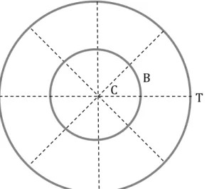
It is assumed that frequency is proportional to supply and that waiting time and changing time are inversely proportional to frequency. We assume the simplified model of the city and its bus line network depicted in Fig. 1.
Fig. 1. Stylized model of city line network.
The largest circle represents the edge of the city, which coincides with the two terminuses of each line (T), and the smallest circle (B) marks the boundary between the inner and outer zones. The straight lines represent the bus routes. Although Fig. 1 gives the impression that changes are only possible in the city center, it is assumed that changing between routes is possible at multiple unspecified points (as in reality, routes are not straight lines). The assumption is that the line network is fixed, and that increases and decreases in supply are made proportional to the original distribution of supply within each time period and zone. It is assumed that net boarding and alighting occur at a constant positive rate (bus stops are not represented in the model) for buses going toward the city center and at a constant negative rate for buses moving outwards. This implies the model of occupancy per bus line depicted in Fig. 2.
C = Center
B = Inner/outer zone boundary T = Terminus
10
Fig. 2. Stylized model of occupancy variation for each bus line in the baseline scenario.
d = Distance
𝑜̅ = Mean occupancy
𝑜̅𝑂 = Mean occupancy in outer zone
QI = Inner passenger flow (person-km/one-way bus)
QO = Outer passenger flow (person-km/one-way bus)
This representation of occupancy represents a simplification, as there are substantial differences in occupancy between bus lines in the same period and the same zone in Uppsala. For our purposes, it is assumed that this representation is sufficient, as the aim here is to examine whether there is potential to adjust frequency. Fig. 3 depicts the real variation in occupancy along Line 1 in Uppsala, which can be compared with the model version shown in Fig. 2.
Fig. 3. Variation in occupancy along Line 1 (in persons/vehicle).
When the number of passengers changes from the baseline, the slope in Fig. 2 changes and the slopes between T and B are allowed to differ from those between B and C. If, in addition, the supply also differs between the inner and outer zones, there will be a kink in the occupancy at B. However, we do not account for the increased number of transfers that this would imply, which is not very realistic. The idea is to provide a hint as to whether there is potential for spatial differentiation of supply. If so, possible means of doing so in practice include
0 5 10 15 20 25 30 PE R S./V EH ICL E
SEQUENCE OF STOPS ALONG LINE 1
C d=0.5 B T Occupancy Distance (Time) 𝑄𝐼 2 𝑜̅ 2𝑜̅ 2𝑜̅𝑂 B T 𝑄𝑜 2
11
shortening or extending some lines, or introducing new, shorter lines. Such measures would require additional analysis on a more detailed route level. Next follows a formal presentation of the central equations. A list of parameters and variables can be found in Appendix B, and a more complete representation of the model can be found in Appendices C and D.
The generalized consumer cost per car trip in each OD pair, time period (TP), and iteration (i) is:
𝐺𝐶𝑂𝐷,𝑇𝑃,𝑖𝑐𝑎𝑟 = 𝐷𝐶∙𝑑𝑂𝐷+𝑝𝑂𝐷,𝑇𝑃𝑐𝑎𝑟 𝑜𝑐𝑎𝑟 + ∑ (𝑉𝑜𝑇𝑧,𝑇𝑃,𝑖 𝑖𝑣𝑡,𝑐𝑎𝑟∙ 𝑡 𝑂𝐷,𝑧,𝑇𝑃,𝑖 𝑖𝑣𝑡,𝑐𝑎𝑟 ) 𝑧 , (2) where 𝐷𝐶 is the distance cost per car (comprising cost of capital, fuel, and wear and tear) and 𝑝𝑂𝐷,𝑇𝑃𝑐𝑎𝑟 is the mean parking fee paid per car, OD pair, and time period.
The generalized consumer cost per PT trip in each zone, time period, and iteration is:
𝐺𝐶𝑂𝐷,𝑇𝑃,𝑖𝑃𝑇 = 𝑝𝑂𝐷,𝑇𝑃𝑃𝑇 + ∑ (𝑉𝑜𝑇𝑇𝑃𝑗,𝑃𝑇 ∙ 𝑡𝑂𝐷,𝑃𝑇,𝑇𝑃𝑗 ) + 𝑗=𝑤𝑎𝑖𝑡,𝑤𝑎𝑙𝑘,𝑐ℎ
+ ∑ (𝑉𝑜𝑇𝑧 𝑧,𝑇𝑃,𝑖𝑖𝑣𝑡,𝑃𝑇 ∙ 𝑡𝑂𝐷,𝑧,𝑃𝑇,𝑇𝑃,𝑖𝑖𝑣𝑡 ), (3) where 𝑝𝑂𝐷,𝑇𝑃𝑃𝑇 is the fare per OD pair and time period, j denotes trip components other than in-vehicle time, 𝑤𝑎𝑖𝑡 denotes the waiting time, 𝑤𝑎𝑙𝑘 the walking time to reach bus stops, and 𝑐ℎ the changing time between bus lines for each trip. The change in number of trips per mode, OD pair, and time period due to a policy reform is (in iteration i):
∆𝐷𝑂𝐷,𝑚,𝑇𝑃,𝑖𝑡𝑜𝑡 = ∆𝐷̃𝑂𝐷,𝑚,𝑇𝑃,𝑖+ ∑𝑚̂ ,𝑇𝑃̂(−∆𝐷̃𝑂𝐷,𝑚̂ ,𝑇𝑃̂ ,𝑖 ∙ 𝜃𝑚𝑂𝐷,𝑚,𝑇𝑃̂ ,𝑇𝑃̂ ) (4) where
∆𝐷̃𝑂𝐷,𝑚,𝑇𝑃,𝑖 = ∆𝐺𝐶𝑂𝐷,𝑇𝑃,𝑖𝑚 ∙ 𝜀𝑚,𝑇𝑃 (5) is the partial change in demand resulting from changes in the own generalized cost of each travel alternative (𝑚, 𝑇𝑃).
∆𝐺𝐶𝑂𝐷,𝑇𝑃,𝑖𝑚 = 𝐺𝐶𝑂𝐷,𝑇𝑃,𝑖𝑚 − 𝐺𝐶𝑂𝐷,𝑇𝑃,0𝑚 (6) 𝜀𝑚,𝑇𝑃 is the own generalized cost elasticity, derived from the own price elasticity.13
𝜃𝑚𝑂𝐷,𝑚,𝑇𝑃̂ ,𝑇𝑃̂ is the share of changes in trips in one alternative (𝑚, 𝑇𝑃) resulting from changes in the generalized cost of another alternative (𝑚̂ , 𝑇𝑃̂ ). For the closest travel alternatives, this is proportional to travel demand in iteration 0, while for 13 𝜀 𝑚,𝑇𝑃= 𝜀𝑚,𝑇𝑃 𝑝𝑟𝑖𝑐𝑒 ∙∑𝑂𝐷(𝐺𝐶𝑂𝐷,𝑇𝑃,𝑖𝑚 ∙𝐷𝑂𝐷,𝑚,𝑇𝑃,0) ∑𝑂𝐷(𝑝𝑂𝐷,𝑇𝑃,𝑖𝑚 ∙𝐷𝑂𝐷,𝑚,𝑇𝑃,0)
12
other travel alternatives, this parameter is zero. That is, the distribution of changes of trips to the three closest alternatives is proportional14 to the number of trips in each of these three alternatives in the baseline scenario.
As a last step, the total number of trips for each travel alternative within each OD pair is updated as:
𝐷𝑂𝐷,𝑚,𝑇𝑃,𝑖+1 = 𝐷𝑂𝐷,𝑚,𝑇𝑃,𝑖+ ∆𝐷𝑂𝐷,𝑚,𝑇𝑃,𝑖𝑡𝑜𝑡 . (7) Eqs. (2–7) are run in a recursive loop (in which 𝑖 is increased by 1 for each iteration) until the system reaches the user equilibrium, which is the first iteration when there is no substantial difference between any variable versus in the previous iteration.
The change in consumer surplus (due to a policy change) compared with baseline is defined by the rule of one-half, for each mode,15 time period, and OD pair (in iteration i), as:
∆𝐶𝑆𝑖 = − ∑ [∆𝐺𝐶𝑂𝐷,𝑇𝑃,𝑖𝑚 ∙𝐷𝑂𝐷,𝑚,𝑇𝑃,𝑖+𝐷𝑂𝐷,𝑚,𝑇𝑃,0
2 ]
𝑚,𝑂𝐷,𝑇𝑃 . (8) The total cost of providing supply in each zone and time period is:
𝑐𝑧,𝑇𝑃,𝑖 = (𝑐𝑑 ∙ 𝑑𝑧𝑙 + (𝑐𝑡 + 𝑘𝑇𝑃,𝑖∙ 𝑐𝑘 ) ∙ (1 + 𝛿𝑧,𝑇𝑃,𝑖) ∙ 𝑡𝑙) ∙
∙ 𝜃𝑧∙ 𝑆𝑧,𝑇𝑃∙ 𝑇𝑇𝑃, (9) where 𝑐𝑑 is the cost per distance for buses (i.e., fuel and wear and tear), 𝑐𝑡 the running cost per hour for buses (i.e., driver wages), 𝑐𝑘 the capital cost per hour for buses, 𝛿𝑧,𝑇𝑃,𝑖 delay due to congestion, 𝑡𝑙 the mean duration of each one-way trip, 𝜃𝑧 the share of the line that is in zone z, 𝑆𝑧,𝑇𝑃 the bus supply in departures per hour, and 𝑇𝑇𝑃 the length of the time period; 𝑘𝑇𝑃,𝑖 is a dummy-type variable16 indicating whether capital cost should be borne by the time period in question (typically 1 for peak and typically 0 for OP).
14 The proportional assumption could be categorized as a naive assumption, due to lack of data.
There is some literature on these cross-elasticities (see Appendix F), but it is our subjective judgment that this literature is too sparse and too little tailored to our specific problem to clearly be better than the naive assumption. Also, the naive assumption has some empirical backing. Flügel et al. (2018) find that cross-modal diversion factors, defined as the proportion of people who leave mode A and switch to mode B, are in general higher for transport modes B with a relatively high market share, consistent with our assumption. It may be reasonable when comparing modes during the same time period, but may be problematic when comparing mode choice with timing choice. The model can easily be updated in this regard as new data on the subject become available. In Appendix H a sensitivity analysis on the cross elasticities is performed, testing the extreme alternative model assumption that travelers can switch between car and PT modes (in the same time period). That is, there is no switching of time period and no switch to walk/cycle. The results imply that total welfare gains from optimization are robust to this alternative model specification.
15 However, there is no change in the generalized costs of walk/cycle, so in practice this calculation is
performed for car and bus transport only.
16 It is not formally a dummy, since in the unexpected event of exactly equal supply in peak and OP
13
The total welfare effect of a given policy change is:
∆𝑊𝑖 = (1 + 𝜇) ∙ ∆𝐶𝑆𝑖 + (1 + 𝜏) ∙ (∆𝑃𝑆𝑖 + ∆𝑃𝑅𝑖) + ∆𝐶𝑇𝑖 + ∆𝐸𝑖, (10) where 1 + 𝜇 is the WEB factor, 1 + 𝜏 is the MCPF factor, ∆𝑃𝑆𝑖 denotes changes in producer surplus, ∆𝑃𝑅𝑖 the total net benefit of changes in parking revenues, ∆𝐶𝑇𝑖 congestion benefits for trucks, and ∆𝐸𝑖 the net social cost of other external effects, all compared with the baseline. It is assumed that all parking lots are publicly owned (simplification) and that parking is marginal cost based;17 that is, the total net benefit of changes in parking revenues is ∆𝑃𝑅𝑖 = 0.
The welfare optima given different restrictions are defined as: max
𝑆,𝑓 (∆𝑊𝑖∗|𝜉, Ѱ), (11) where 𝑆 and 𝑝 are two-dimensional matrices, 𝜉, Ѱ are a set of restrictions, and 𝑖 ∗ denotes the user equilibrium.18 𝑆 has the dimensions time period and zone, while 𝑓 has the dimensions time period and OD pair.
𝜉 ∈ {𝑝𝐼−𝑂,𝑇𝑃∗
𝑃𝑇 ≥ 𝑝
𝐼−𝐼,𝑇𝑃𝑃𝑇 ∗ 𝑝𝐼−𝑂,𝑇𝑃𝑃𝑇 ∗ ≥ 𝑝𝑂−𝑂,𝑇𝑃𝑃𝑇 ∗
for each time period, 𝑇𝑃∗.
Thus, within each time period it should not be cheaper to travel in both zones compared to just one.
Ѱ ∈ ∅ defines the welfare optimum.
Ѱ ∈ {𝑆 = 𝑆0 defines the optimum given fixed supply. Ѱ ∈ {𝑝 = 𝑝0 defines the optimum given fixed fares.
Ѱ ∈ {∆𝐺𝐶𝑂𝐷,𝑇𝑃,𝑖∗𝑚 ≤ 0 defines the optimum given the restriction of Pareto improvements from the baseline for all 𝑂𝐷, 𝑚, 𝑇𝑃, (“Pareto scenario”).
The robustness and uniqueness of optima in BUPOV are discussed in Appendix E, which shows that there are no indications that any optimum is not robust and unique.
3 DATA
Uppsala lies 70 kilometers north of Stockholm (Sweden’s capital) and has one of Sweden’s oldest universities. In 2010, it had 155,000 inhabitants and its urban
17 In the sensitivity analysis, the alternative assumption that the marginal revenue is only half of the
marginal cost has been tested; that is, that ∆𝑃𝑅 = − ∑ 𝑝𝑂𝐷,𝑇𝑃𝑐𝑎𝑟 ∙ (
∆𝐷𝑂𝐷,𝑐𝑎𝑟,𝑇𝑃,𝑖 𝑜𝑐𝑎𝑟 )
𝑂𝐷,𝑇𝑃 . The results
indicate that the welfare gains from optimization are robust in this dimension.
18 Note that eq. (11) implies that the policy maker is a Stackelberg leader, setting policy in
anticipation of the future total response (in the last iteration only). That is, policy is set once only and not in every iteration i.
14
area covered 51 square kilometers; this urban area was served by a network of city buses with 22 lines covering the city.19 Table 2 summarizes descriptive data on Uppsala’s PT service.
Table 2
The urban bus services in Uppsala in 2010; SEK 1 ≈ EUR 0.1.
Total number of lines 22
Total net route length 430 km
Trips (boarding passengers) 15.7 million
Total cost SEK 336 million
Fare revenue SEK 176 million
Source: Public Transit Department UL (RPTA).
According to a 2010 travel survey, the mode share (per trip) of PT was 11 percent of trips within Uppsala (Uppsala Municipality, 2016), quite high compared with several smaller cities (Pyddoke and Swärdh, 2017), but low compared with Sweden’s larger cities (Norheim et al., 2017).
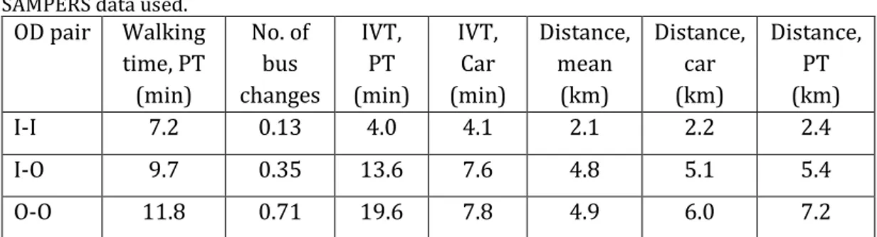
The BUPOV model is calibrated using travel data from the national travel surveys and from the Swedish national passenger demand model, combined with boarding data from the RPTA. In addition, a more accurate representation of parking fees is applied based on current local regulations.
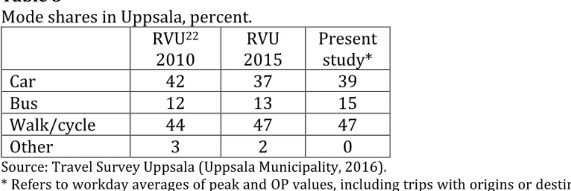
One difference from the travel survey is that this study concerns workdays only. Another is that in addition to trips within the city, we also include trips with an origin or destination outside of Uppsala (see Appendix H: Calibration). In this study, the distribution of trips across modes, OD pairs, and time periods is taken from the Swedish national travel demand model, SAMPERS.20 This model is regularly updated for the purpose of national infrastructure planning. We have used data from 2010 as a baseline.21 Because the absolute numbers in the SAMPERS data do not coincide with those from the municipality’s travel survey for 2015 (Uppsala Municipality, 2016) and boarding data from 2014 (UL, 2015), the SAMPERS demand predictions have been scaled to fit the boarding data. For the number of trips, see the baseline column in Table I1 in Appendix I. Table G1 in Appendix G reports other SAMPERS data that were used. Table 3 reports the mode shares for Uppsala.
19 A large network reform reducing the number of routes to 14 was enacted on 14 August 2017. 20 The use of SAMPERS data, the data aggregation, and the representation of congestion and
crowding in PT were inspired by the HUT model used by Pyddoke et al. (2017).
15 Table 3
Mode shares in Uppsala, percent. RVU22
2010 2015 RVU Present study*
Car 42 37 39
Bus 12 13 15
Walk/cycle 44 47 47
Other 3 2 0
Source: Travel Survey Uppsala (Uppsala Municipality, 2016).
* Refers to workday averages of peak and OP values, including trips with origins or destinations outside Uppsala.
The distribution of producer costs between staff, capital, and wear and tear is taken from Eliasson (2015). These costs are then scaled up (by about 1.2) to coincide with the actual total costs of PT in Uppsala in 2010 (from the official accounting by Public Transit Department UL, RPTA; see Table 4).
Table 4 Costs per bus.
SEK/year SEK/h SEK/km Eliasson (2016) 426,177 285 7.7 Present study 531,363 355 9.5
BUPOV uses (own) generalized cost elasticities, calibrated to match empirical own price elasticities; see Table 5.23
Table 5
Elasticities of demand with respect to (own) price and generalized cost (GC) in present study.
Mode Price elasticity from
Time
period elasticity Price Price/GC in baseline Resulting GC elasticity Car Börjesson et
al. (2017) Peak OP –0.54 –0.85 76% 75% –0.71 –1.14 PT Balcombe
(2004) Peak OP –0.26 –0.48 25% 24% –1.06 –2.00
Street congestion data are from Tomtom (2017). Costs of crowding and congestion, and the marginal cost of public funds are taken from the Swedish national guidelines on the welfare economics of infrastructure investments, ASEK 6 (Swedish Transport Administration, 2016). The marginal external effects of traffic safety, emissions, and noise from cars and buses (including
22 RVU = Resvaneundersökning = Travel habit survey.
16
internalization) are calculated for Uppsala based on a combination of ASEK 6, Nilsson and Johansson (2014), Swedish Transport Administration (2015), and ASEK 3 (SIKA, 2005).24 According to these calculations, car trips in Uppsala have internalization rates (for all calculable externalities except congestion) of slightly more than 100 percent, while emissions from buses are only internalized by about 50 percent (see Table 6). This means that there will be a small welfare gain from an increased number of car trips, not counting the congestion externalities, since the extra tax collected is worth more than the costs of all other externalities including the emission caused, and vice versa for the buses.
Table 6
Internalization rate of emissions. Car Bus
Inner 104% 50% Outer 119% 55%
Additional data are reported in Appendix G.
4 RESULTS
In this section, four policy scenarios are analyzed (see eq. 11 in Section 2). Marginal results are available in Appendix I. In the first scenario, Fares only, fares for each zone and time period are chosen to optimize welfare. In the second,
Supply only, frequencies are chosen for each time period and OD pair to optimize
welfare. In the third, Welfare optimum, fares and frequencies are chosen simultaneously to optimize welfare (without restrictions). Finally, in the Pareto
scenario, a further restriction is added: no consumer group (mode, period, or
zone) is allowed to have its generalized cost per trip increased. Table 7 shows the resulting optimal levels of the policy variables.
24 In Samkost (Nilsson and Johansson, 2014), total externality per vehicle-km was SEK 0.22 for cars
and SEK 1.64 for heavy vehicles (e.g., buses) on average in Sweden; however, the authors used a somewhat lower CO2 emission value than the official one (ASEK 6). Because this figure is both
difficult to estimate and controversial, we have chosen the official figure and have adjusted the Samkost values in this respect. We have also adjusted for local conditions in Uppsala compared with the national averages for noise (data from Samkost), NOX, and particulate matter emissions
(emission factors from the Swedish Transport Administration, 2015; Uppsala-specific valuations from ASEK 3). We have also accounted for the fact that roughly 40% of the buses run on biogas. These adjustments increased the total externality per vehicle-km to SEK 0.38 for cars in the outer zone, SEK 0.43 for cars in the inner zone, SEK 1.86 for buses in the outer zone, and SEK 2.05 for buses in the inner zone in Uppsala. The total tax (from Samkost) is SEK 0.45 for cars and SEK 1.02 for buses.
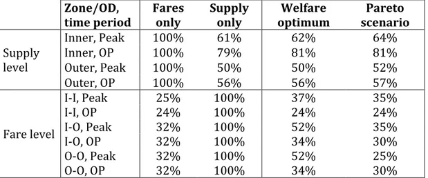
17 Table 7
Optimal policy parameter values25 with different restrictions (as percent of baseline).
Zone/OD, time period Fares only Supply only optimum Welfare scenario Pareto Supply level Inner, Peak 100% 61% 62% 64% Inner, OP 100% 79% 81% 81% Outer, Peak 100% 50% 50% 52% Outer, OP 100% 56% 56% 57% Fare level I-I, Peak 25% 100% 37% 35% I-I, OP 24% 100% 24% 24% I-O, Peak 32% 100% 52% 35% I-O, OP 32% 100% 34% 30% O-O, Peak 32% 100% 52% 25% O-O, OP 32% 100% 34% 30%
The estimates presented in Table 7 indicate that the optimal policy involves reductions in both fares and supply For the fares and supply in the outer zone, the reductions are drastic. The optimal reductions in supply range from 19 percent (OP hours in the inner city in the Welfare optimum and Pareto scenarios) to 50 percent (peak in the outer zone in the Supply only scenario and Welfare optimum) and are generally larger in the outer zone than in the inner zone. The table also shows that optimal supply differs less between scenarios than do optimal fares. Optimal fares depend more on supply than vice versa, that is, the welfare function for each set of restrictions appears to be flat with respect to fare level.
Table 8 shows the effects in terms of aggregate demand for each mode. Table 8
Changes in number of trips in the examined optima versus baseline (in percent). Mode Base-line
trips
Policy scenario (optima) Fares
only Supply only optimum Welfare optimum Pareto
Car 133,881 -4% +3% -1% -1%
PT 50,920 +23% -15% +6% +8%
WB* 161,372 -4% +2% -1% -2%
* WB = Walk/cycle
The fares only and supply only scenarios lead to considerable changes in PT demand, while in the welfare and Pareto optima the aggregate effects are smaller. However, these aggregate demand changes hide larger changes for the various OD pairs and time periods.26 The relative effects on car trips and WB are rather small, simply because car and WB trips exceed PT trips in total numbers.
25 Best candidate found for global optimum for each set of restrictions.
26 In the welfare optimal scenario, PT demand increases substantially for inter and I-I trips in OP
18
Table 9 shows the effects of the policy scenarios (Table 7) and the respective changes in travel alternatives (summarized in Table 8) on congestion (delay) and crowding (occupancy).
Table 9
Delays (compared to free-flow conditions) and occupancy in buses in baseline and in the examined optima, respectively.
Zone Time period Mode Baseline
Policy scenario (optima) Fares
only Supply only optimum Welfare scenario Pareto Delay
Inner Peak Car+PT 96% 91% 93% 90% 89%
OP Car+PT 42% 39% 42% 39% 39% Occupancy (pers./vehicle) Inner Peak PT 62% 69% 93% 99% 100% OP PT 48% 61% 52% 67% 67% Outer Peak PT 27% 30% 50% 53% 53% OP PT 21% 27% 30% 40% 40%
Table 9 shows that congestion is modestly affected, while there are large effects on bus occupancy rates in the three scenarios in which supply is reduced. The occupancy increases the most in peak hours: from around 60 percent to around 100 percent in the inner zone and from around 30 percent to around 50 percent in the outer zone. Table 10 shows the effects on financial outcomes for the RPTA. Table 10
Financial outcomes for RPTA in SEK per workday and changes in subsidy level and capacity use due to different policy scenarios; the figures are expressed as changes versus baseline.
Financial outcome Baseline Fares only Supply only Welfare optimum Pareto scenario Fare revenue 572,515 –355,672 –86,870 –338,902 –382,881 Producer costs 1,232,885 –10,851 –514,806 –515,309 –501,032 Producer surplus –660,370 –344,821 +427,936 +176,408 +118,150 Capacity use in OP 67% 0% +12% +12% +10%
Optimizing welfare with lower fares imposes large costs on the RPTA in terms of lost revenue, which is counteracted by somewhat decreased costs due to shorter rotation times of vehicles due to reduced congestion. There is, however, an
frequency dominates the effect of lower fares, so demand decreases. In the Pareto scenario, PT demand increases for all I-I and inter trips pairs in both time periods, but the number of O-O trips is constant compared to baseline.
19
interesting potential to optimize supply. The results indicate that doing so may reduce costs by about 40 percent, suggesting substantial current excess supply. The capacity use in OP is substantially improved in the three scenarios in which supply is optimized. Next, Table 11 presents the implications in terms of total welfare.
Table 11
Welfare social costs (negative sign) and benefits (positive sign) in SEK per workday of different policy scenarios; the figures are expressed as changes versus baseline.
Welfare effect Fares only Supply only optimum Welfare optimum Pareto Consumer surplus +465,202 -247,753 +100,770 +166,696 From which congestion benefits +39,062 +8,346 +40,424 +44,922 Producer surplus –344,821 +427,936 +176,408 +118,150 MCPF + WEB –47,622 +98,651 +65,015 +55,449 Other external benefits* +363 +7,143 +7,303 +7,104
Net social benefits
(SEK) +73,123 +285,976 +349,496 +347,399
* Net benefits of external effects and taxation of external effects, including congestion benefits for trucks.
Three observations stand out. First, substantial improvements in social welfare can be gained by reducing supply in the Supply only scenario. Second, in terms of net welfare, optimization of the Fares only scenario does not achieve much compared to the Supply only scenario. Third, in the Pareto scenario, social welfare can be improved without reducing generalized costs for any identified group (travelers by any mode, for any OD pair, in any time period) in the model. This comes at a cost of a SEK 2,000/workday loss in social welfare compared with the welfare-optimal scenario, which is small compared with the producer cost of SEK 1,200,000/workday in the baseline scenario.
A sensitivity analysis was also performed with respect to ten key parameters or assumptions (see Appendix J). For most of the parameters tested, the idea has been to challenge the main finding that frequency of service should be reduced. For example, the consequence of a lower MCPF was tested (using 1.12 instead of 1.3), although from an empirical point of view a larger MCPF (of maybe 1.5) seems more likely. However, since using a WEB factor is not standard procedure, the model was tested by removing it. This change shows that reducing supply improves welfare even more than the baseline. In three instances the model was
20
tested to its limits (Table J3).27 The results indicate that model uncertainty (model limitations) is not more important than parameter uncertainty.
The welfare gain of baseline optimization appears to be robust throughout the sensitivity analyses, perhaps with a few exceptions. In the most sensitive case, (where we assume that the values of waiting time are 50 percent higher than in the base model), there is still a considerable welfare gain due to optimization, even if optimizing according to erroneous parameter estimates.
The directions of changes in optimal supply and price levels are as expected. The supply recommendations seem robust and supply reductions are smaller in the inner zone than in the outer zone (smallest reduction for inner zone in OP) in all tests. Optimal fare levels are non-robust, but peak fares are higher than OP fares in all cases (they are equal only when all fares are 0). The results for the MCPF = WEB = 1.2 and parking cost scenarios stand out, in that they prescribe free PT. However, even for these scenarios, the model prescribes a reduction of supply, although not as large as in the base model.
5 DISCUSSION
The main aim of this study is to analyze welfare-optimal fares and frequencies differentiated in time and space in Uppsala, a small Swedish city, and to compare different scenarios with alternative goal functions. The most important finding is that optimization of supply indicates a current large oversupply of bus service in Uppsala, mostly in the outer parts of the city. This implies that the RPTA can make substantial savings while still improving welfare. If the supply planning routines in other small cities are similar to Uppsala’s, large welfare improvement may be possible there also. According to the Swedish Association of Local Authorities and Regions (SKL, 2014, Diagram 5), Uppsala Region’s mean occupancy of 8.5 passengers/vehicle is in the lower half of the distribution among regions in Sweden (the mean is 11 passengers/vehicle). On the other hand, the result of reducing supply in off-peak periods is in line with Börjesson et al. (2017), who conducted a similar analysis of a corridor in Stockholm, Sweden’s largest city with the largest PT share. Stockholm Region has the second highest mean occupancy level in Sweden (according to Diagram 5 in SKL, 2014). Proost and Dender (2008) and Savage (2010) found that PT frequencies were too high in London, Brussels and Chicago. However, Basso and Silva (2014) and Tirachini et al. (2014) estimated substantial increases in PT frequencies would be optimal in London, Santiago, Chile and Sydney. These results indicate that findings are situation specific and may be hard to generalize. Hower, the diverging resluts for London between studies indictate that different modeling approaches (different policy aspects included or not) may be imortant in explaing the differenes.
27 First, it was tested by removing street congestion from the model, to see how important street
congestion is to the results. Second, the assumption that passengers are evenly distributed in each direction of the line was tested by examining the opposite extreme: that all passengers travel in the same direction. Finally, it was tested to impose extreme assumptions about cross-elasticities, to examine whether the simple cross-demand model in BUPOV seems reasonable.
21
The results suggest that RPTAs should be careful when dimensioning their supply. The simplicity of the BUPOV model makes it possible to perform analogous analyses without extensive costs. The sensitivity analyses suggest that in Uppsala the welfare losses that result from optimizing with a model which includes some errors28 are small compared to the welfare gains of using optimization as a tool in practice. If this is also true for other cities, there is a large potential for optimizing PT supply in midsized cites worldwide.
The total welfare is rather insensitive to fare changes, while these changes have large distributional effects, both among consumers and between the region (financing the RPTA) and the consumers as a group. The results indicate that the optimal supply level is only marginally affected by the different model assumptions and has large effects on total net welfare, while welfare-optimal levels of fares are both sensitive to changes in model assumptions and less important (from an aggregate welfare point of view).
The results are also in line with those of Börjesson et al. (2017), namely, that an optimal policy involves peak pricing, that it is optimal to subsidize PT to some extent, and that optimization of frequency is more important than optimization of fares. However, the results differ in that the results of Börjesson et al. (2017) for Stockholm suggest that increased fares during peak hours would increase welfare, whereas the results of the present analysis of Uppsala suggest that reduced fares in the inner zone during peak hours would increase welfare.29 This difference between the studies’ results may be due to less initial crowding on buses combined with the fact that street congestion is not priced in Uppsala. That is, low PT fares may partly work as a second-best substitute for congestion charges. The sensitivity analysis with respect to congestion suggests that the congestion in Uppsala reduces the optimal prices by between 10 and 40 percent, which should be of similar order as the second-best effect in this respect.
The sensitivity analyses indicate that optimizing PT fares in an urban setting is sensitive to the basic assumptions about the MCPF and about the social costs and benefits of parking. It is also important to have good data on the costs and benefits of parking, and there is currently a lack of good estimates of demand elasticities and costs. An interesting expansion of the present study would be to examine the implications of the optimization of parking fees on optimal PT fares.
In the present study, two welfare optima with respect to supply and fares respectively have been analyzed, one of which was an unrestricted welfare optimum, while the other was given the restriction that the aggregate generalized cost should not increase for any OD pair, time period, and mode combination. Both optima involve a reduction in supply and fares. Of the two, the Pareto scenario may seem more attractive as most of the large total gains in the welfare optimum can be achieved without any consumer group being worse off in terms
28 The sensitivity analysis also suggests that demand model uncertainty is not more important than
parameter uncertainty.
29 Basso and Silva (2014) also found it optimal to reduce fares for the larger cities of London and
22
of generalized travel cost than in the baseline scenario. Also, in the Pareto scenario, the total number of PT trips increases substantially (and there are also some additional environmental benefits). We can see that from an environmental perspective, it is more effective to decrease fares than to increase supply. This is because the fare reduction attracts travelers to the PT mode and hence reduces the emissions from cars, without increasing the emissions from buses. Here there is obviously a trade-off between crowding on buses and the environmental benefits. In the present study, this trade-off was balanced with the welfare weights implied by the shadow prices in the national guidelines.
There is one caveat to the normative conclusion that supply should be reduced in Uppsala, namely, that we do not have detailed data on occupancy variation. We therefore cannot exclude high variance in occupancy, which could justify some degree of oversupply compared to average occupancy, in order to provide capacity when demand is high. However, the sensitivity analysis suggests that taking some degree of variation in demand into account would not eliminate the potential for supply reduction to improve welfare.
Finally, it is important to keep in mind that BUPOV uses a representative line approach. The model suggests that frequency should be reduced on average, but since the number of travelers varies across lines, it is possible that for the most utilized lines it would be optimal to keep the high frequencies or even increase them.
ACKNOWLEDGMENTS
This study was financed by K2 – The Swedish Knowledge Center for Public Transport; the Centre for Transport Studies, Stockholm; and Vinnova, Sweden’s innovation agency. We thank Urbanet Analys AB for generously supplying SAMPERS OD-matrix data aggregated to zones, and Stefan Adolfsson and colleagues at the Public Transit Department UL for comments. We also wish to thank Maria Börjesson and Karin Brundell-Freij for their excellent reviewing and comments, and Stef Proost for inspiring discussions of how to model congestion and public transport in cities.
23
REFERENCES
Anderstig, C., Berglund, S., & Börjesson, J. (2018). Regionalekonomiska effekter av planförslagen 2018–2029: Beräkningar med Samlok-modellen, Version: 0.1, Trafikverket, Borlänge.
Balcombe, R. (editor), Mackett, R., Paulley, N., Preston, J., Shires, J., H. Titheridge, & Wardman, M. (2004). The demand for public transport: A practical guide. TRL Report 593.
Basso, L.J., Guevara, C.A., Gschwender, A. & Fuster, M. (2011). Congestion pricing, transit subsidies and dedicated bus lanes: Efficient and practical solutions to congestion. Transport Policy, 18(5), 676–684.
Basso, L.J., & Silva, H.E. (2014). Efficiency and substitutability of transit subsidies and other urban transport policies. American Economic Journal: Economic
Policy, 6(4): 1–33. http://dx.doi.org/10.1257/pol.6.4.1
Beckman, M., McGuire, C. B., & Winsten, C. B. (1956). Studies in the Economics of
Transportation. New Haven, Conn.: Yale University Press.
Börjesson, M., Fung, C.M., & Proost, S. (2017). Optimal prices and frequencies for buses in Stockholm. Economics of Transportation, 9, 20–36, ISSN 2212-0122. https://doi.org/10.1016/j.ecotra.2016.12.001
Eliasson, J. (2015). Förbättrade metoder för samhällsekonomisk analys av
kollektivtrafikinvesteringar. CTS Working Paper 2016:6.
Eliasson, J., & Fosgerau, M. (2017). Cost‐benefit analysis of transport improvements
in the presence of spillovers, matching and an income tax. CTS Working
Paper 2017:3.
Flügel, S., Fearnley, N. & Toner, J. (2018). What factors affect cross-modal substitution?: Evidences from the Oslo Area. Int. J. Transp. Dev. Integr.,
2(1), 11–29, ISSN: 2058-8313 (online),
http://www.witpress.com/journals, DOI: 10.2495/TDI-V2-N1-11-29 Halvorsen, A., Koutsopoulos, H. N., Lau, S., Au, T., & Zhao, J. (2016). Reducing
subway crowding: Analysis of an off-peak discount experiment in Hong Kong. Transportation Research Record: Journal of the Transportation
Research Board, No. 2544, Transportation Research Board, Washington,
24
Jennervall, P. (2016). Så mycket kostar bilförsäkringen där du bor. Expressen, 2016-12-21, https://www.expressen.se/motor/sa-mycket-kostar-bilforsakringen-dar-du-bor/
Jussila Hammes, J., Pyddoke, R., & Swärdh, J. E. (2016). The influence of public
transport supply on private car use in 17 midsized Swedish cities from 1997 to 2011. CTS Working Paper 2016:25.
Kilani, M., Proost, S., & van der Loo, S. (2014). Road pricing and public transport pricing reform in Paris: Complements or substitutes? Economics of
Transportation, 3:175–187.
Kleven, H., & Kreiner, C. (2006). The marginal cost of public funds: hours of work versus labor force participation. J. Public Econ. 90(10–11),1955–1973. Mohring, H. (1972). Optimization and scale economics in urban bus
transportation. American Economic Review, 62 (4), 591–604.
Nilsson, J.-E., (2011). Kollektivtrafik utan styrning?, report to subcommittee to Swedish ministry of finance.
Nilsson, J.-E., & Johansson, A. (2014). SAMKOST—Redovisning av
regeringsuppdrag kring trafikens samhällsekonomiska kostnader. VTI
rapport 836.
Norheim, B., Pyddoke, R., Betanzo, M., Haug, T.W. (2017). Komparativa analyser Stockholm, Göteborg, Malmö och Uppsala, Urbanet Analyse Notat 2016/90.
OECD (2019). Urban population by city size (indicator). doi: 10.1787/b4332f92-en (Accessed on 26 March 2019).
Parry, I. W. H., & Small, K.A., 2009. Should urban transit subsidies be reduced? American Economic Review, 99(3): 700–724. DOI: 10.1257/aer.99.3.700 Proost, S., & van Dender, K. (2008). Optimal urban transportation pricing in the
presence of congestion, economies of density and costly public funds.
Transportation Research Part A: Policy and Practice, 1200–1230.
Pyddoke, R. & Swärdh, J.-E. (2017). The influence of demand incentives in public
transport contracts on demand and costs in medium sized Swedish cities. K2
working paper 2017:10.
Pyddoke, R., Norheim, B. & Fossheim Betanzo, M. (2017). A model for strategic
planning of sustainable urban transport in Scandinavia: a case study of Uppsala. CTS sworking paper 2017:7.
25
Savage, I. 2010 The dynamics of fare and frequency choice in urban transit Transportation Research Part A, V 44, pp. 815–829.
SIKA. (2005). KALKYLVÄRDEN OCH KALKYLMETODER (ASEK)—En sammanfattning av Verksgruppens rekommendationer 2005, SIKA PM 2005:16.
SKL. (2014). Öppna jämförelser – Kollektivtrafik 2014, Sveriges Kommuner och Landsting, ISBN 978-91-7585.
SKL. (2017) Kollektivtrafikens kostnadsutveckling: en överblick, Sveriges Kommuner och Landsting, ISBN 978-91-7585-529-5.
Swedish Transport Administration. (2015). Handbok för vägtrafikens
luftföroreningar, Bilaga 6.1. http:
//www.trafikverket.se/TrvSeFiler/Fillistningar/handbok_for_vagtrafike ns_luftfororeningar/kapitel_6-bilagor_emissionsfaktorer.pdf
Swedish Transport Administration. (2016a). Analysmetod och samhällsekonomiska kalkylvärden för transportsektorn: ASEK 6.0.
Swedish Transport Administration (2016b). Prognos för persontrafiken 2040— Trafikverkets basprognoser 2016:059, ISBN 978-91-7467-942-7.
Tirachini, A, Hensher, D.A. & Rose, J.M. (2014). Multimodal pricing and optimal design of urban public transport: The interplay between traffic congestion and bus crowding. Transportation Research Part B, 61, 33–54.
Trafikanalys. (2016). Swedish national and international road goods transport
2015, official statistics.
Tomtom. (2017). www.tomtom.com/en_gb/trafficindex/city/UPP, Accessed January 30, 2017.
UL. (2015). Statistisk årsbok 2014—Kollektivtrafiken i Uppsala län, Landstinget i Uppsala län – Kollektivtrafikförvaltningen UL.
Uppsala Municipality. (2016). Resvaneundersökning hösten 2015 – En
kartläggning av kommuninvånarnas resmönster hösten 2015.
Vickrey, W.S. (1963). Price and resource allocation in transportation and public utilities: pricing in urban and suburban transportation. American
26
Vigren, A., & Ljungberg, A. (2018). Public Transport Authorities’ use of cost-benefit analysis in practice. Research in Transportation Economics, 69, 560–567, ISSN 0739-8859, https://doi.org/10.1016/j.retrec.2018.06.001 Wardman, M.J., & Ibáñez, N. (2012). The congestion multiplier: Variations in motorists’ valuations of travel time with traffic conditions. Transportation
27
APPENDIX A: A QUADRATIC UTILITY FUNCTON
Consider the following utility function of a representative consumer: additively separable, quadratic in the quantity of each travel option, 𝑞𝑖, and linear in other generalized consumption, 𝑐 (including leisure), as in Börjesson et al. (2017):
𝑢 = 𝑐 + ∑ [𝑎𝑖𝑞𝑖 − 0.5𝑏𝑖𝑞𝑖2]
𝑖 (A1)
𝑐 = 𝑦 + 𝑝𝐿𝐿 − ∑ 𝑝𝑖 𝑖𝑞𝑖 𝑞 = ∑ 𝑞𝑖 𝑖
where 𝑦 is income, 𝑝𝐿 is the price of leisure, 𝐿 is leisure, 𝑝𝑖 is the generalized cost of option 𝑖, and 𝑞 is total travel demand; 𝑎𝑖, 𝑏𝑖 𝑦, 𝑝𝐿, 𝐿, and 𝑞 are constant, 𝑝𝑖 is a non-choosable variable, and 𝑞𝑖 is an optimization variable for the representative individual.
When 𝑢 is maximized subject to 𝑞𝑖, the following holds: 𝜕𝑢
𝜕𝑞𝑗= −𝑝𝑗− ∑ [𝑎𝑖− 𝑏𝑖𝑞𝑖
]
𝑖≠𝑗 = 0 (A2)
Differentiating with respect to 𝑝𝑖 gives (after simplification): 𝜕𝑞𝑗
𝜕𝑝𝑗 = −1 − ∑ [𝑏𝑖 𝑖] (A3)
B3 implies: i. 𝜕𝑞𝑗
𝜕𝑝𝑗 is constant, i.e., a linear demand function.
ii. 𝜕𝑞𝑗
𝜕𝑝𝑗 =
𝜕𝑞𝑖
𝜕𝑝𝑖 for all 𝑖, 𝑗.
Note: i. is conistent with demand modeling and consumer surplus calculation (rule of one-half) in BUPOV; however, ii. may be too restrictive in practice.
28
APPENDIX B: NOTATION
𝐴𝑧 Area of zone (Inner, outer) CS Consumer surplus
CT Congestion costs for trucks 𝐷 No. of trips, demand
𝑑 Distance (OD, travel distance, route) 𝛿 Delay (percentage)
𝑐 Cost of supply, i.e., per km, per hour, per capacity (capital cost), in total
𝑆𝐶 Seating capacity of each bus
𝐷𝐶 Distance cost of car (inner, outer, fixed)
𝐸 Total net external effect, excluding congestion (PT, car; inner, outer) 𝑒 Net external effect per vehicle-km, excluding congestion (PT, car;
inner, outer)
𝜀 Elasticity
𝑓 Frequency
𝐹𝐶 Fixed cost per trip (i.e., devaluation for car, fixed cost of changing vehicles, and walking time for PT)
𝐺𝐶 Generalized consumer cost/trip 1 + 𝜇 Wider economic benefits factor (WEB) 𝑜 Occupancy (mean, point; car, PT) 𝑝 Fare (PT), parking fees (car) 𝑃𝑆 Producer surplus
PR Parking revenue
𝑄 Flows (Person, vehicle per hour; eq. per area and hour) 𝑟 Revenue from fares
𝑆 Supply (departures per hour) 𝑇𝑇𝑃 Length of period (peak, OP)
𝑡 Travel time, i.e.,, in-vehicle time (IVT), changing time, and waiting at home
1 + 𝜏 Marginal cost of public funds factor (MCPF)
𝑉𝑜𝑇 Value of time (IVT, changing time, waiting at home, trucks, and PT supply)
W Total welfare
𝛾 Level of subsidy (result)
Ѱ Set of restrictions for welfare optima Super- and subscripts
Modes (m): car, public transport (PT), and walk/(bi-)cycle (WB) Zones (z): Inner = I, Outer = O
OD pairs (OD): I-I, I-O, and O-O
Locations (L): Center = C, Boundary inner = BI, Boundary outer = BO, and Terminus = T
Time period (TP): peak (P), off-peak (OP) Model iteration (MI): i