Estimating Erosion in Oil and Gas Pipe Line Due to Sand Presence

Full text

(1)Master's Degree Thesis ISRN: BTH-AMT-EX--2011/D-16--SE. Estimating Erosion in Oil and Gas Pipe Line Due to Sand Presence. Akar Abdulla. Department of Mechanical Engineering Blekinge Institute of Technology Karlskrona, Sweden 2011 Supervisor:. Ansel Berghuvud, BTH Gustavo A. Zarruk, IFE, Norway.

(2)

(3) Estimating Erosion in Oil and Gas Pipe Line Due to Sand Presence Akar Abdulla Department of Mechanical Engineering Blekinge Institute of Technology Karlskrona, Sweden 2011 Thesis submitted for completion of Master of Science in Mechanical Engineering with emphasis on Structural Mechanics at the Department of Mechanical Engineering, Blekinge Institute of Technology, Karlskrona, Sweden. Abstract: Transporting solid particles in oil and gas flow cause erosion damage to the pipeline and fittings. The aim of this thesis is to study the effect of impact velocity on the erosion damage in 90 degree long elbow by using two different erosion models namely, Oka model and E/CRC model. Those correlation applied at air-borne sand eroding, methane-borne sand eroding, mixed gas-borne sand eroding, and multiphase (gas- oil) borne sand eroding Inconel 625. The commercial computational fluid dynamics (CFD) code STAR-CCM+ is used to obtain the average and maximum erosion rate by using the above mentioned models and compared them with the previous results. Keywords: CFD, Erosion, Solid particle impact, Multiphase flow , Turbulence. 1.

(4) Acknowledgements This work was performed as part of the FACE centre (Multiphase Flow Assurance Innovation Centre), research cooperation between IFE, NTNU, and SINTEF. The centre is funded by The Research Council of Norway, and by the following industrial partners: Statoil Hydro ASA, GE Oil & Gas, Scand power Petroleum Technology AS, FMC, CD-Adapco, and Shell Technology Norway AS. I would also like specially acknowledge CD-Adapco for providing a license of their software, STAR-CCM+, and Dr. Martin Kempf and the entire CDAdapco technical support team for their help during this work. This work was carried out under supervision of Dr Ansel Berghuvud at the Department of Mechanical Engineering, Blekinge Institute of Technology, Karlskrona, Sweden, and Dr Gustavo A. Zarruk at the Institute for Energy Technology (IFE), Kjeller, Norway. First, I would like to express my sincere gratitude to Dr Ansel Berghuvud for his guidance and support during the work and providing the computer to carry out the thesis. I wish to thanks Dr Gustavo A. Zarruk and the Institute for Energy Technology (IFE) for supporting this work. Finally, I would like to express very special thanks to my parents who have supported, encouraged, and inspired me throughout whole my life. And I am grateful to thanks all my friends. Karlskrona, December, 2011 Akar Abdulla. 2.

(5) Contents 1 Notation. 5. 2 Introducitons. 9 . 2.1 Aim and scope. 10. 3 Literature Review on Erosion Models. 11 . 4 Mathematical Modelling Theory. 17 . 4.1 Multiphase Flow. 17. 4.2 Continuous Phase Flow Modelling. 18 . 4.3 Dispersed Phase Flow Modelling. 18 . 4.4 Conservation Equatuions. 19 . 4.4.1 Conservation of Mass. 19 . 4.4.2 Conservation of Momentum. 19 . 4.4.3 Conservation of Energy. 22 . 4.5 Euler-Lagrange approach. 23. 4.6 Euler-Euler approach. 24. 4.7 Volume of Fluid (VOF) Multi-phase Model. 25 . 4.8 Lagrangain Multiphase Modelling. 25 . 4.9 Turbulence Modelling. 27 . 4.9.1 Reynolds-Averaged Naveir-Stoke (RANS). 27 . 4.9.2 K-Epsilon (K ε) Turbulence. 28 . 4.9.3 Realizable Two-Layer K-Epsilon Model. 29 . 4.9.4 Two Layer All y+ Wall Treatment. 32 . 4.10 Summary of Equations. 33 . 5 Erosion Modelling. 36 . 5.1 Erosion. 36. 5.2 OKA Erosion Model. 36 . 5.3 E/CRC Erosion Model. 38 3.

(6) 5.4 Coefficient of Restitution (COR). 39 . 6 Computational Fluid Dynamic Simulations. 41 . 7 Results. 50. 8 Discussion, Conclusion and Recommendations. 93 . 8.1 Discussion. 93. 8.2 Conclusion. 95 . 8.3 Recommendations. 96 . 9 References. 98. Appendix A. 100. Average Erosion rate in an inlet and outlet pipe. 4. 100.

(7) 1. Notation C. Constant Drag coefficient Lift coefficient Constant Constant Model coefficient. c. Speed of sound. D. Constant. d. Diameter ′. ⁄. Reference diameter ,. E. Particle diameter Energy Erosion damage at normal angle Erosion damage at arbitrary angle. ⁄ ⁄. Drag force Lift force TD. Turbulent dispersion force. VM. Virtual mass force Particle shape coefficient Turbulence kinetic energy product due to the mean buoyancy. ⁄. Turbulence kinetic energy product due to the mean ⁄. velocity Gradients Gravitational vector g. Acceleration due to gravity 5. ⁄.

(8) The ratio of erosion damage at arbitrary angle to normal angle ⁄. H. Enthalpy. Hv. Vickor’s hardness [Gpa] Unit matrix ⁄ . °C. Diffusion heat flux ,. ,. Exponent constants Effective conductivity. m. ⁄ . °C. Mass Mass of flow Mass of particle. n. Exponent power ,. p. ,. Exponent constants ⁄. Pressure. ⁄. Tangential cutting pressure. ,. Normal cutting pressure. ⁄. Time averaged pressure Exponent constants. ⁄. Reynolds number Reynolds number for dispersed flow r. Radius of spherical particle Strain rate tensor 1⁄ Means module strain rate tensor 1⁄. S ,. Constant Response time of particle Time averaged velocity Velocity gradient 1⁄. 6. ⁄.

(9) ⁄. Continuous phase velocity. ⁄. Dispersed phase velocity. ⁄. Particle impact velocity. Relative velocity between continuous and dispersed phase ⁄ ′. ⁄. Reference velocity. Rotation rate tensor 1⁄ W. Constant. x. Constant. y. Constant. z. Constant. Greek letters Volume fraction Thermal expansion coefficient ∆. Volume loss Turbulent dissipation rate. ⁄. Particle impact angle Dynamic viscosity of the continuous phase ⁄ .. Turbulent viscosity. Continuous phase density Flow density Gas density. ⁄. ⁄ ⁄. Liquid density Particle density. ⁄ ⁄ ⁄. Reynolds stresses. Turbulent Prandtl number for kinetic 7. ⁄ ..

(10) Turbulent Prandtl number for energy Stress tensor. ⁄. ⁄. Constant Temperature gradient vector °C Abbreviations CFD. Computational Fluid Dynamics. COR. Coefficient of restitution. DES. Detached Eddy Simulation. DNS. Direct Numerical Simulations. LES. Large Eddy Simulation. RANS. Reynolds-Averaged Navier-Stokes. RSM. Reynolds stress model. TKE. Turbulence kinetic energy. TDE. Turbulence energy dissipation. VOF. Volume of Fluid. 8.

(11) 2. Introduction This work was performed as part of the FACE centre (Multiphase Flow Assurance Innovation Centre), research cooperation between IFE, NTNU, and SINTEF and in co-operation with Blekinge Institute of Technology in Sweden. In the oil and gas industry, the extracted oil and gas from the well is inevitable polluted with solid particles such as sand, solid particle and sand in particular is a source of several flow assurance problems. One of them is erosion damage to pipeline, fittings (e.g., elbows and, chocks chocks), and several other control equipment. If erosion is not properly monitored, predicted and controlled, entire production processes can be hampered and even shut down for extended periods of time. Understanding of wearing in pipe material and control equipment material caused by sand impinge is necessary either for protecting pipeline and equipments against potential hazard and/or for designing pipeline and equipments. Estimating sand erosion is a very complicated phenomenon in a multiphase phase flow and there are a variety of factors which have an effect on the erosion damage (e.g., impact velocity, impact angle, and size of particle, shape of particle, properties of particle, and properties of the target material). In order to obtain erosion predictions caused by sand particles, many investigations have been carried out to develop empirical and numerical the erosion models. This thesis was performed as part of the FACE centre, research cooperation between IFE, NTNU, and SINTEF. In this thesis, a computation fluid dynamics (CFD) based erosion model was applied to estimate the average and maximum erosion rate in a 90 degree elbow. The simulations modelled by using STAR-CCM+ to estimate erosion in multiphase flow. Four different cases are studied more precisely air-sand, methane-sand, and mixed gas-sand two-phase flow , while for the fourth case oil-gas-sand three-phase flow are used to predict maximum and average erosion rate by using two different models namely the Oka model and E/CRC model. In the first case the maximum and average erosion rate are obtained on the whole 90 degree long elbow and ER probe which is installed at four degree above and under 45 degree at the outer of the 90 degree elbow. The 9.

(12) dimension of the ER probe is (0.0142 * 0.0364 meter). Then the results compared with the previous experimental and CFD based predicted erosion. Meanwhile, for the remaining case the maximum and average erosion rate are obtained only in a 90 degree elbow.. 2.1 Aim and Scope Gaining more knowledge about estimating erosion rate in multiphase flow is one of the main purposes of this thesis. The scope of the present work is to focus on how particle impact velocity has big influence the maximum and average erosion rate in a long 90 degree elbow when sand particles flow in a different continuous flow. And also to study the effect of using different kinds of continuous phases (Air, Methane, Mixed gas, and OilGas) with different densities on the maximum and average erosion rate and the location of erosion rate and the location of erosion rate.. 10.

(13) 3. Literature Review on Erosion Models Basically, erosion is caused by impact of solid particles (sand) which is suspended in flow (liquid, gas or multiphase flow) on a solid wall or boundary. In other words, it can be described as gradual removal of material by repeated deformation and cutting action [1]. Figure 3-1 shows the relationship between particle impact angle and erosion ratio for brittle and ductile materials.. Figure 3-1 the relationship between Erosion rate and impact angle for brittle and ductile materials. Finnie for the first time proposed the cutting mechanism “wear which occurs when solid particles entrained in a fluid stream strike a surface” [2].. 11.

(14) sin 2. 6 6. 6. 3.1. 6. is the volume of material removed by single particle, is the Where particle mass, is the particle velocity, is the constant plastic flow stress, is the particle impact angle, is the ratio of the force component ( vertical force to horizontal force), and is the ratio between depth of contact and cut which is equal to 2. Then after that, Bitter proposed another mechanism based on the wearing and deformation on the surface caused by particles [3], [4]. According to Bitter’s mechanism, the cutting process happens when the particle impact the surface of material with a relatively small impact angle, that cause the particles remove a small amount of surface material by scratching on it. In contrast, the deformation process happens when particles impact the surface of material with a relatively big impact angle. That cause micro crack on the surface material and surface fragmentation. Equation 3.3 shows the total volume erosion rate which is a summation of volume erosion rate by deformation and cutting mechanism respectively. 3.2 1 2 2. ′. 3.3 ′. 3.4. Where, is the total volume erosion rate, and are the volume of material removed by deformation and cutting mechanism respectively, M is the particle mass, V is the particle velocity, is the particle impact angle, is the particle impact angle at the time when horizontal component of velocity reach zero after leaving particle from the body, is the threshold velocity, and are particle and target module of 12.

(15) elasticity, is the threshold velocity, and are wear factors needs to be found experimentally, and from equation 3.4 are constants and can be found by using below equations (equations 3.5 and 3.6). ′. 0.288. 3.5 1. 1. 0.82. 3.6. Then, Bitter model was simplified by Neilson and Gilchrist [5]. The simplified model for ductile erosion model by them can be seen in the equation 3.7 as; cos 2 cos 2. 2. 3.7 2. Where W is the total removed volume of the targeted material. Finnie’s model for erosion later was modified by Hashish [6]. In Hashish’s model, the effect of the shape of particle was considered. Additionally, the velocity exponent was modified and set to 2.5. Equation 3.8 shows Hashish’s model for erosion; .. 7. sin 2 3. 3.8. √sin. ⁄. 3.9. Since then, a lot of researchs have been done to improve the erosion equation and tried to obtain the equation which has the majority of the factors has an effect on erosion rate. Meng and Ludema [7] described 28 various erosion wear models and equations in their article. 13.

(16) Equation 3.10 shows another model which is used by Hutchings, in this model the critical strain is used as a function of material removal while the velocity exponent is set to 3[8]. .. 0.033. 3.10. ⁄. Ω. Where is the romval material, is the constant plastic flow stress, is the hardness of target, and Ω is the critical strain [7]. The Nelson and Gilchrist model was developed by Wallace et al in that model the cutting and deformation wear coefficient were introduced and used in to the model. The model has two formulas which depend on the impact angle either greater or smaller than 45° . Habib and Badr [9] used the Wallace et al model and compared with experimental result. Their results showed that the velocity has a big impact on erosion rate. Brenton S. McLaury [10], investigates the computational and experimental data of the elbow and tees. It was demonstrated that continuous phase has a significant effect on erosion rate. C. Huang [11], developed model which includes both deformation and cutting mechanism, the models (equation 3.11) includes the effect of abrasive particles, target material and particle size. The model shows a good agreement with both Finnie and Bitter experimental data. Δ. ⁄ ⁄. Dm. ⁄. sin ⁄ ⁄. ⁄. V d. ⁄. cos θ. ε PP. sin θ. ⁄. 3.11. ⁄. Where ∆ is the volume loss, is the particle mass, is the particle density, is the particle velocity, is the particle impact angle, is the elongation of target material, and are the tangential and normal cutting pressures during cutting process, respectively, C and D are constants, the exponent b can be obtained experimentally, and the exponent n is the shape factor. In this equation, the first term of the right-hand side 14.

(17) represent deformation wear while the second term represents the cutting wear. This works show that the relation between erosion and impact velocity on the cutting removal while the particle size has a weak influence on cutting removal. The particle impact angle in the straight pipeline flow or even slightly curved pipeline flow is very small and the particle moves nearly parallel to the surface of pipeline because the flow direction does not change a lot. So in this case the particles approach the pipe wall due to turbulence fluctuation and gravitational force. However, in the fittings like elbow, headers, or tees there is a direct particle impact angle-relatively big impact angle- on the wall of the elbow, headers or tees. 3.12 Equation 2.12 represents one of the equations of erosion of particle which is based on the impact angle and impact velocity. Where, ER is erosion rate, is particle impact velocity and is particle impact angle. This equation shows that the erosion rate has power-law relation with particle velocity, and in this equations the value of n- velocity exponent- for metallic material is typically lie down between 2 and 3 [11]. 3.13 Equation 3.13 is given by McLaury and Shirazi [13], in this equation the factor -particle shape coefficient-introduced to the equation. The value is equal to 1 for sharp (angular), 0.53 for semi-rounded, or 0.2 for fully rounded sand particle. And the particle impact angle defined as:. 3.14. sin. Where a, b, w, x, y, z, and are empirical constants which depends on the targeted materials. McLaury and Shirazi [13] used this model to compare the computational and experimental result. It was noticed that the particle rebound model may have an effect on particle trajectory. 3.15 Equations 3.15 is another general form of empirical correlation for 15.

(18) estimation erosion where, K, , , and are constants and depends on the particle and targeted materials properties, While V, d, and C represent velocity, particle diameter, and solid concentration. Girish [14] used equation 3.15 for studying the erosion rate for seven different ductile materials. Their investigation shows that the erosion rate depends on the particle velocity and particle size. It was also noticed that the ratio between erodent material hardness to target material hardness has an effect on the erosion rate in ductile materials at normal impact condition. In another word, erosion rate is a function of ratio between erodent material hardness to target material hardness. 3.16 An equation 3.16 was used by Ahmed Elkholy, where k, m, n, and p are constants for pipe material and flow and Rajact Guta [12] experimentally found the value of those constants and finally two equations were obtained for brass and mild steel. 0.178. .. 0.223. . .. 3.17. . .. .. 3.18. Where V is the particle velocity, d is the particle diameter and is the concentration by weight. In equation 3.17 and 3.18, it can be seen the velocity exponent between 2 and 3 and it has a big effect on erosion. Oka et al. erosion [1], [15] and the E/CRC (Erosion Corrosion Research Centre) by Zhang [16] separately developed erosion model and those models will be discussed in the next chapter.. 16.

(19) 4. Mathematical Modelling Theory. 4.1 Multiphase Flow Multiphase flow is defined as any system of flow consisting of more than one phase for example a mixture of gases, liquids, and/ or particles, drops, or bubbles. In multiphase flow, liquids and gases are dealt with as separated flow and on the other hand particles, drops, or bubbles are dealt with as dispersed phase [17]. Multiphase flow can be classified into four groups which are: 1. Liquid-liquid or liquid gas flows; example of this category is bubbly flow, slug flow, droplet flow. 2. Liquid-solid flows, example of this category is slurry flow- when particle transporting in liquid. 3. Gas-solid flows, example of this category is particle laden flow which particles are dispersed flow with continuous flow (gas flow). 4. Three phases flows; this category could be the combination between the three above categories. For example it could be liquid-gas-solid or liquid-liquid-solid. In oil and gas production, commonly multiphase flow occurs in a different stage of the production, starting from extracting oil and gas from wells and transporting through pipelines. There are several approaches for modelling multiphase flow, the most accurate and available in CFD codes are, Eulerian model, Lagrangian model, and volume of fluid (VOF) model. In this work, two different category of multiphase based on the multiphase classification are studied in terms of number of the phases. In the first case, two phase gas- solid is investigated; in this case the governing equation for continuous fluid phase (gas) is expressed in Eulerian form and the dispersed phase (solid particles) is modelled by using a Lagrangian method. In the second case, three phases gas-liquid-solid is investigated; in this case for modelling the continuous phases (gas and liquid) volume of flow (VOF) model is used. However, Lagrangian method is used for dispersed phase (sand particles) in the same manner as it is used in the first case. 17.

(20) 4.2 Continuous Phase Flow Modelling All the computational method depends on the mathematical formulas which are describe the flow. The general mathematical formula of the continuous phase is, conservation equation including mass conversation, and momentum and those equations can be described by Navier-Stoke equations. However, calculating turbulence has to take in consideration since it has big influence on the solution and it has to be dealt with by modelling the turbulence flow which is called turbulence modelling.. 4.3 Dispersed Phase Flow Modelling Dispersed multiphase flows occur in a different kind of industrial process, petroleum field is one of them. Dispersed phase consist of finite number of particles, drops or bubbles distributed in a connect volume of the continuous phase. Commonly, there are two models to deal with dispersed phase, trajectory models and two fluid models [17]. In the trajectory model, the Lagrangian approach can be used to predict the trajectory of particles by integrating the force balance (drag force, lift force and moment force) on the particle. However, in the two fluid models, the Eulerian approach can be used for modelling and in this approach, the dispersed phase is dealt with as a secondary continuous phase and there is an interacting with the other continuous phase and the equations can be solved for both continuous and dispersed phase. There is another issue needs to be addressed which is called coupling. Coupling needs to be done between continuous and dispersed phase, there are four kinds of coupling which are Ono-way coupling, Two-way coupling, Three-way coupling, and Four-way coupling. When the concentration of the dispersed phase is very small compare to continuous phase, then the effect of dispersed phase can be ignored this is called Oneway coupling. However, if there is an interaction between the continuous and dispersed phase and the dispersed flow can effect on the continuous flow, this is Two-way coupling. In this thesis two way coupling is used. And there is Three-way coupling in which has an additional interaction when the particle disturbance of the fluid in the dispersed phase affects the 18.

(21) motion of the particles. And finally, the Four-way coupling in which has an additional interaction when the collision between particles in dispersed phase affects motion of individual particles.. 4.4 Conservation Equations 4.4.1. Conservation of mass. The general equation of conservation of mass can be described by equation of mass balance for the fluid element. It can be written as: .. 4.1. 0. The first term and the second term of the equation 4.1 represent the rate of change of density in time- the rate of increase of mass- (mass per unit of volume) and the net rate of flow of mass out of fluid element. Where, is the volume fraction, is the number of phase (liquid, gas, and solid), and is the partial derivative of quantity with respect to all direction. The summation of must be equal to 1. 1. 4.4.2. 4.2. Conservation of momentum. The general form of the conservation of momentum (Newton’s second low) describes that the rate of change of momentum of a fluid particle equals to the sum of the forces acting ton that particle [18]. It can be expressed as: . p. .. .. 4.3. .. 4.4 19.

(22) For two phases (gas and liquid) . p .. 4.5. . p. 4.6. .. Where, is the volume fraction and is the number of phases (liquid, gas, and solid). The summation of must be equal to 1, is the pressure and its assumed to be equal in all phases, is molecular stress, is turbulent stress, is inter-phase momentum exchange (per unit of volume). Mass conservation and momentum conservation equations together are known as Navier-Stoke equations. The inter–phase momentum transform includes drag force, virtual mass force, lift force and turbulent dispersion force. Equation 4.7 shows the summation of those forces and the formula of each one of them can be expressed as follow; VM. TD. 4.7. Drag force: Is the force that generate by interaction between solid particle and surrounding fluid. Drag force has two sources; skin friction and form drag. Skin friction is related to shear stresses of the solid particle (skin of solid particle) when interacts with fluid, and dependent on the viscous friction between particle and fluid. Form drag or (pressure drag) which arises due to normal stress and it 20.

(23) depends on the shape of the solid particle. Equation (4.8) shows the drag force equation by Gosman. 3 CD | | ρα d 4. 4.8 4.9. Where, is a drag force, is the relative velocity between dispersed and and are dispersed and continuous phase velocities continuous Phase, respectively, c and d subscripts represent continuous and dispersed phase respectively, d is the particle diameter which is represent the interaction length between the continuous and dispersed flow, and CD is the standard drag coefficient for spherical particles and its calculated by Schiller and Naumann as: CD. 24. 1. 0.15. .. 0. 0.44. 1000. 4.10. 1000 d | |. 4.11. Where, is the dynamic viscosity of the continuous phase. Reynolds number of dispersed flow.. is the. Virtual mass force: Virtual mass force or sometimes called added mass force is the additional force required to accelerate particle and part of the fluid surrounded by it. This force has a significant effect when the density of the dispersed phase is less than the density of continuous phase. The equation of virtual mass flow is: 4.12. VM. 21.

(24) and. Where. are material derivative for the dispersed phase and is a virtual mass coefficient and its. continuous phase respectively. And equal to 0.5 [20]. Lift force:. Lift force is the force which is perpendicular on the velocity direction of the flow. 4.13 4.14 Where,. is the lift coefficient and equal to 0.25.. Turbulence dispersion force: Turbulence dispersion force is arise due to interaction of the solid particles with the liquid eddies. The combination of turbulence eddies and interphase drag are cause turbulence dispersion force which take place between two regions of high and low volume fraction. For instance, in dispersed phase turbulence cause particle to be moved from the high concentration region to low concentration region. Equation 4.15 shows the turbulence dispersion force equation. TD. 3 CD v | | ρα 4 d σ. 4.15. α. Where, v is the continuous phase turbulent kinematic viscosity, and σ is the turbulent Prandtl number, Prandtl number is a dimensionless number and it’s the ratio between the momentum diffusivity (kinematic viscosity) and thermal diffusivity. 4.4.3. Conservation of Energy. The general equation of conservation of Energy or the first law of the thermodynamics in which declares that the rate of change of energy of a 22.

(25) fluid particle is equals to the rate of heat addition to the fluid particle the rate of work done on particle [18] and it can be written as: . T. .. 4.16 h. .. There are four terms on the right hand side of equation 4.16. The first term represents the heat transfer due to conduction or diffusion. While the second term represents the species diffusion heat transfer. The third term represents heat loss due to viscous dissipation. And the last term represent the general source that might include radiation or other sources. 4.17 2 mh. 4.18. T. 4.19. C dt. h T. Where, E is the energy, h is the enthalpy, p is the pressure, v is the magnitude velocity, is the effective conductivity, is the diffusion heat flux, is the stress tensor, and is the velocity gradient.. 4.5 Euler-Lagrange approach In this approach, the fluid phase is dealt with as a continuous phase by solving the Time-Averaged Navier-Stokes equations. On the other hand, the dispersed phase is solved by tracing large number of particles, droplets, or 23.

(26) bubbles trajectories through the domain of the calculated flow. The dispersed phase has an effect on continuous phase and this effect be represented by the force which is applied at the dispersed phase. Mass, momentum, and energy can be exchanged in the dispersed phase with continuous phase. As it was mentioned, the particle trajectories are dealt with individually in the flow domain and the second dispersed phase occupies a low volume fraction despite of the difference in the mass loading in case of the mass of particle is greater than the mass of fluid. In this approach, to obtain a realistic coupling –two way coupling-between two phases (continuous flow and particles) it’s necessary to track a large number of particles which computationally make to use this approach very expensive especially if the two way coupling is considered between continuous flow and particles. Modelling the particle flow interaction, collision, and wall interaction are main advantage of using this approach. However, that makes the computational cost high.. 4.6 Euler-Euler approach Euler-Euler approach and also called two-fluid mode is one of the approach to simulate continuous and dispersed phase numerically. In this approach every phases are dealt with as a continuous phase and conservation equations apply for each phase to derive a set of equations. The conservation equations for two-fluid are derived from the conservation equation for mass, momentum, and energy which govern the behaviour of each continuous phase. After applying an averaging to the whole twophase system, the conservation equations for the two-fluid are obtained. The volume fraction of the phases are introduced which are considered as a continuous functions of the space and time. The summation of these volume fractions is equal to one. There are different Euler-Euler multiphase models for modelling multiphase flow such a volume of fluid (VOF), multiphase segregated flow, the mixture model, and the Eulerian model.. 24.

(27) 4.7 VOF Multi-phase model Volume of Fluid (VOF) is a simple and most common approach for modelling several immiscible fluids. In this model one set of momentum equations is solving for all phases and the volume fraction of each of the fluids in any computational cell is tracked through the domain and also all phases has the same velocity, pressure and temperature. The volume fraction in each cell is equal to zero when there is not fluid (empty cell) in that cell. However, this value is equal to one for the cell full of fluid (occupied cell). When there is an interface between fluids in a cell the value is between 0 and 1.. 4.8 Lagrangian Multiphase modelling In multiphase simulation, usually the fluid phase is treated as a continuous phase and governed by Eulerian frame. And this carries numerous dispersed phase which is called parcel and each one of them is modelled in Lagrangian frame. Each parcel represents a number of identical particles having the same properties such as a size. The trajectory of each percale can be predicted and the governing equation can be solved by using the Lagrangian multiphase modelling which is also known as a Lagrangian model. The particle conservation equation of momentum is known as particle equation of motion and also this equation is also known as BBO equation which was used by Basset, Booussinesq, and Oseen [19]. 4.20 4.21 4.22 4.23 Where and are surface and body force on the particle respectively. While , , , , , are drag force, pressure force, virtual mass force, gravity force, lift force, and turbulent dispersion force 25.

(28) respectively. is the dispersed phase velocity (particle velocity), is the mass of dispersed phase (particlemass), and the left side of the equation 4.20 is summation of the force action on the particle. Drag, lift, virtual mass and turbulent dispersion forces were shown previously, the pressure and gravity force can be written as; 4.24 4.25 is the continuous phase velocity and vector.. is the gravitational acceleration. The Lagrangian equation governing the motion particle can be written as: 4.26 3 CD | | ρα 4 d 4.27 3 CD v | | ρα 4 d σ. α. Where, is the total acceleration of the continuous phase, and derivative with respect to time. 4 3. is the 4.28. 4 3. 4.29. Where, r is the radius of the particle, and the relation between can be written as: 26. and.

(29) 4.30 On the right side of equation 4.27, six terms can be identified, the first term represent the drag force which is the most dominant force on the particle motion. The second term represents the pressure gradient force due to the acceleration of the surrounded continuous phase. The third term represents the added mass force (virtual mass), which is an additional force due to inertia force because the continuous phase surrounding the particle is accelerated as well. The fourth term represents lift force. The fifth term represents turbulent dispersion force and the last term represents the gravity force.. 4.9 Turbulence modelling Generally, turbulence can be defined as a time dependent chaotic of flow which can be seen in almost all flows. There are several approaches to model turbulence in CFD, the most reliable and common approaches are, Reynolds-Averaged Navier-Stokes (RANS), Large Eddy Simulation (LES), Detached Eddy Simulation (DES), and Direct Numerical Simulations (DNS). In this thesis the Reynolds-Averaged Navier-Stoke (RANS) is used for modelling turbulences. The aim of this model is to obtain Reynolds stress model which can be done either by using Eddy Viscosity model (liner and nonlinear), or Reynolds stress model (RSM). The idea behind of Eddy Viscosity model is using turbulence viscosity to model Reynolds stress. The Reynolds stress can be modelled by using kepsilon model, k-omega model, Reynolds Stress Transport, Smagorinsky Subgrid Scale Turbulence or Spalart-Allmaras. Here in this thesis, the Kepsilon model is used for modelling Reynolds stress. 4.9.1. Reynolds-Averaged Navier-Stoke (RANS). Reynolds-Averaged Navier-Stoke (RANS) equations are time averaged equations for the fluid motion. (RANS) can be used as a basis of modelling many Two-equation models including K-Epsilon and K-Omega model. 27.

(30) Reynolds decomposition is the idea behind RANS equations, where timeaveraged part can be separate from fluctuating parts of quantities. In other word, it means that the turbulence flow can be analysed and dealt with two component, mean component and fluctuating component. This can be seen in the equations below for velocity and pressure: ′. 4.31. ′. Where and. and are time averaged velocity and pressure respectively, while are velocity and pressure fluctuating component.. After that these transform can be expressed as a set of unknown which is called Reynolds Stresses or sometimes called Reynolds stress tensor. This is a function of the velocity fluctuations required for turbulence modelling such as a k-Epsilon or K-Omega. . p. .. 4.32. .. ′. ′. ′. ′. 2 3 2 3. 4.33. . .. 2 3. 4.34. Where is the Reynolds stress, is the turbulent viscosity and k is the turbulent kinetic energy, . is the velocity divergence, and is the unit tensor. 4.9.2. K-Epsilon (K- ) Turbulence. The K -Epsilon (K- ) turbulence model is one kind of the Two-equation model for predicting the behaviour of the turbulent flow. And it is one of the most popular models. Where K is the kinetic energy and is the dissipation rate of the turbulent energy, and the model transport equations 28.

(31) are solved for those to quantities. K- Model is one of the most general used in the CFD codes and it has been used in a several form in many industrial applications. In this model, conservation equations for both turbulence kinetic energy and dissipation rate are solved besides Navier-Stokes equation of the flow. Since it was found by A.N. Kolmogorov, it has been a lot of attempts to improve the model and make it applicable for the variety range of problems. Nowadays there are several K- models available for instance, Standard K-Epsilon, Standard Two layer-K-Epsilon, Standard LowReynolds number, Realizable K-Epsilon, and Realizable Two-Layer KEpsilon. 4.9.3. Realizable Two-Layer K-Epsilon model. The Realizable Two-Layer K-Epsilon model is a combination of Realizable K-Epsilon model and Two Layer approach. In the realizable k-Epsilon model, the model consists of new transport equation for the turbulence can be seen that is expressed dissipation rate . The coefficient of model as a function of mean strain, mean flow, rotation rates, and turbulence properties. However, this coefficient is assumed to be a constant and equal to 0.09 in K-Epsilon standard model. And K-Epsilon model can be applied in the viscous sub-layer by using Two-layer approach. In realizable K-Epsilon model, the transport equation for K is the same as standard KEpsilon. However, there is a different in transport equation for . The Turbulence kinetic energy (TKE) is given by:.. .. 4.35. S , And the Turbulence Energy Dissipation (TED) can be expressed as:-. 29.

(32) . . 4.36 √. ,. 4.37. , ,. 4.38. Where is the turbulent viscosity and is the model coefficient, is the is the turbulent Prandtl turbulent Prandtl number for kinetic –k-, and number for energy- -. On the other hand, , , and determined by setting the values of coefficients and are coefficients and set to 1.2 and 1 respectively, and using the following equations:√. 4.39. ,. 1 2. 4.40. ,. 4.41. √6. ,. 1 cos 3. √6. 4.42. ,. 4.43. , | |. √2. max 0.43,. √2 5. 4.44. ,. 4.45. ,. 30.

(33) 4.46. , 0 0. 1 0. 4.47. Where is the strain rate tensor, is the module of means strain rate tensor, is the rotation rate tensor, , , and are constants and equal to1.9, 1.2, 1.0, and 4 respectively. ′. 4.48. ′. is the product of turbulence kinetic energy due to the mean Where, velocity gradients and it can be rewritten as; 4.49. , 2 3 2 3. 2 3. . .. :. 4.50. , 2 3. :. ,. 4.51. Or it can be written as 2 3. .. 2 3. 4.52. .. While, is represents the product of turbulence kinetic energy due to buoyancy and it can be found as: 4.53. . Where: 1. 4.54. Where is the thermal expansion coefficient, and is the temperature gradient vector. 31. is the gravitational vector,.

(34) Finally, dilatation dissipation follow [20];. is modelled by using Sarkar model, as 4.55. Where, is constant and equal to 2, and c is the sound speed. be zero for incompressible flow. 4.9.4. is set to. Two Layer All y+ Wall Treatment. In turbulence flow, the presence of walls has a significant effect on flows turbulence because of the fluid have zero velocity relative to the solid boundary (no-slip condition), and has large gradients in the solution variables in this viscosity-affected region.. Figure 4-1 near wall layer subdivision. Figure 4-1 shows the subdivision near wall layer. It can be seen that the boundary layer is divided into inner region and outer region. And the inner region layer divided into three sub-layer as: 1. Viscous sub-layer (or laminar layer. 5). 2. Buffer layer or blending region ( the range between 5 3. Fully turbulent or log-law region (the range between30 60). 32. 30).

(35) In the viscous sub-layer, it’s assumed to , while the fully turbulent or log-law region is described by the logarithmic-liner variation of the nondimensionless velocity. wall treatment is a set of near wall modelling assumption Two layers all for K-Epsilon turbinate model. Where is the dimensionless wall wall parameter and used to describe how the mesh is coarse or fine, all treatment works as a high wall treatment for coarse meshes which is suitable when the near-wall cell in the logarithmic region of the boundary layer. And the low for fine meshes which only suitable for low Reynolds number. Even it could be used for the range 5 30 (buffer layer or blending region).. 4.10 Summary of Equations Final equation of conservation of mass .. 4.26. 0. Final equation of continuous phase momentum is: . p .. 4.57. 33.

(36) Inter-phase force term is: 3 CD | | ρα d 4. 3 CD v | | ρα 4 d σ. 4.58 α. Final dispersed phase momentum equation is:. 3 CD | | ρα 4 d. 3 CD v | | ρα 4 d σ. 4.59. α. 34.

(37) Turbulence kinetic energy (TKE) can be written as: . . 4.60 √. And, turbulence energy dissipation (TED) can be expressed as: . .. √ 4.61. 35.

(38) 5 Erosion Modelling 5.1 Erosion The erosion ratio is defined as the loss of inner wall pipe mass caused by erosion to the mass of particle impacting the wall. Most of the erosion prediction equations are empirical and they are based on experimental data for solid particles in continuous flow (gas or liquid). It is well known that the particle impact velocity and particle impact angle are the principal variables affecting the erosion mechanism. In this thesis project, the Oka and E/CRC models are chosen to estimate erosion rate in a 90 degree elbow because after obtaining erosion rate by using STAR-CCM+, the results will be compared with the experimental and CFD predicted results in the previous work [16]. The previous word done by E/CRC, after conducting experimental, the results compared with the CFD results by using the model which developed by them (E/CRC) and with the Oka model. And also the Oka model is built in method for estimating erosion in the software. Meanwhile, the E/CRC model implemented in to the software to obtain the CFD result by using both models.. 5.2 Oka Erosion Model. Figure 5-1 Repeated plastic deformation and cutting wear action with impact angle (Oka [1]). 36.

(39) 5.1. , sin. 1. ′. 1. sin. ,. 5.2 5.3. ′. Where:. 2.3. ,. 5.4. ,. 5.5. .. 5.6. The idea behind this model is that the impact angle adopted which is the ratio of erosion damage at arbitrary angle to the erosion damage at normal angle . Where K, k1, k2, k3, s1, s2, q1, q2, n1, and n2 are constants and exponent values for particles material and targeted material. [1, 15, 21] The equation of function -equation 5.2- is a combination of two terms. The first term is repeated plastic deformation (brittle characteristics) and the value of this term increase by increasing the particle impact angle. On the other hand, the second term is cutting wear action which has the biggest value when the particle impact is equal to zero and this term more effective in a small angles. Both repeated plastic deformation and cutting wear action can be seen in figure 5-1. In this model, three different kinds of particle were tested with different particle size diameter, density and Hv (Vicker’s Hardness). At the same time different kinds of targeted materials with different density, and Hv were used. In this thesis Silica four (Sio2) is used for particle material, which has density of 2650 ⁄ . The targeted material is Inconel 625 with Vickor’s hardness 3.43 Gpa (BH-Brinell Hardness is equal to 331) and density is equal to 8200 ⁄ . All the above constants and exponents can be seen in table 4-1.. 37.

(40) Table 5-1 constants and exponent for Oka model equations. Particle. Silica four-sio2 0.71 0.14 2.4 -0.94 0.8437222954 0.7534158785. K. 65 -0.12 2.410288411 0.19 104. ⁄. 326. 5.3 E/CRC Erosion Model This model is developed by E/CRC (Erosion Corrosion Research Centre) [16] and the computational result compared with the Oka model and with the experimental data which was carried out by the E/CRC. The experimental data carried out for both direct impact test (ER probe at 12.7 mm distance away from nozzle jet) and 90 elbow erosion test when the ER probe installed in the middle of outer the 90 degree elbow. This model shows a good agreement with both experimental data and the Oka model. The equations of this model are as follow: 5.7. .. 38.

(41) 5.4. 10.11 1.42. 10.93. 6.33. 5.8. Where C is the constant and equal to 2.17 10 , BH is the Brinell hardness, Vp is the particle impact velocity, and Fs is the particle shape coefficient and its equal to 1 for sharp angular, 0.53 for semi-rounded, and 0.2 for fully rounded, is the particle impact angle. The Brinellhardness in this thesis for Inconel 625 is equal to 331 (Hv=3.43 Gpa) [22] and nvelocity exponent- is equal to 2.41.. 5.4 Coefficient of Restitution (COR) Coefficient of restitution is the ratio of the particle velocity component after impact to the particle velocity component before impact. It is used to predict the rebound angle of the particle after hitting the wall. Coefficient of restitution needs to be addressed to predict the particle trajectory accurately. The reflecting velocity usually smaller than the incoming velocity until it reached to zero that means the particle is not rebound from the wall. The process of decreasing velocity occurs due to transferring energy between the particles and wall. Coefficient of restitution depends on several factors such a type of target material, and the impact angle [22]. There are some relationships for coefficient of restitution. Grant and Tabakoff based on some experimental data presented perpendicular and parallel restitutions coefficient [13]. Forder et al. [23] developed a relationship for normal and tangential restitution coefficient for both normal (perpendicular) and tangential (parallel) to the velocity component. Equations below show the Forder relationship for coefficient of restrictions. 1. 0.78. 0.988. 0.84 0.022. 0.78 0.19 0.0027. 0.21. 0.024. 39. 0.028. 5.9. 5.10.

(42) One the other relationship for coefficient of restitution is stochastic rebound model by Grant and Tabakoff. 0.998. 1.66. 2.11. 0.67. 0.993. 1.76. 1.56. 0.49. 5.11 5.12. In this thesis, the coefficient of restitution used was the one developed by Forder et al – equation 5-9 and 5-10-were used [22].. 40.

(43) 6. Computational Simulations. Fluid. Dynamic. Computational fluid dynamics (CFD) for four cases in the 90 degree elbow were simulated by using STAR-CCM+. The 90 degree elbow has the diameter of 0.0508 m with a curvature ⁄ is equal to 1.5. In this thesis, four cases were investigated to estimate the average erosion rate in 90 degree elbow. The first case is simulated when the air was used as the continuous phase. The second case Methane was used as a continuous phase, the third case mixture of gases (91% of Methane (CH4), 5.6% of Propane (C3H8), 1.6% of Nitrogen (N2), 1.3% of Butane (C4H10), 0.3% of Carbon Dioxide (CO2), and 0.2% of Helium (He)) was used as the continuous phase. While, for the fourth case, gas (Methane) - oil (Dodecane- C12H26) were used as a continuous phase. In all cases sand particle was used as dispersed phase. The sand erosion modelling in CFD is consists of four primary steps; grid generation, flow solution, particle track calculation and erosion rate calculation. The STAR-CCM+ contains all the features that are importance for erosion problems.. Figure 6-1Gemoetry of elbow.. 41.

(44) Figure 6-2 Schematic of 90 degree elbow.. Figure 6-3 symmetry of 90 degree elbow. Figure 6-1 shows the geometry 90 degree elbow which was created by using 3D-CAD modeller in the STAR-CCM+. The advantage can be taken of the symmetry of the geometry 90 degree elbow to reduce computing. The symmetry of the 90 degree elbow geometry can be seen in figure 6-3. Then, the CAD model is ready for the next step which is mesh generation. Generally, meshing is consists of two parts; the first part is Surface meshing and the second part is Volume meshing. Generation of surface mesh should be considered very carefully because it has a direct effect on the quality of 42.

(45) resulting volume mesh. Because of this reason, more care is taken during preparation of surface mesh; the better quality will be the resulting of volume mesh. After obtaining the volume mesh, Mesh diagnostics can be run to check the quality of the created mesh. It is very important to choose the most suitable mesh cell size because having a big cell size, the accurate result will not be able to obtain. On the other hand, very small cell size need more iterations to solve the solver equation since each equation run in each mesh cell to gain one single output at the end, eventually the CPU time and memory size decrease by increasing the cell number. The volume mesh for 90 degree elbow was created by choosing polyhedral mesher, prism layer mesher, surface remesher and extruder mesh. The latter was used to create 0.2 m length pipe on both sides of the elbow. Finally, the grid system is suited to model flow domains in all mentioned cases. The surface remesher was picked to improve the overall quality of surface mesh and to optimize the surface mesh for generating volume mesh. Furthermore, the polyhedral mesher was chosen to fill the volume inside the surface mesh and that is the area which solver equations are work in. Polyhedral mesh is preferred rather than tetrahedral mesh because of building polyhedral mesh is easier and more efficient than tetrahedral mesh and it has five times fewer cells than tetrahedral mesh [20]. Usually each cell of polyhedral mesh has an average of 14 cell faces. Finally, the prism layer was used to obtain an accurate result next to wall boundaries because it is very important to simulate the turbulence accurately next to the wall boundaries. Figures 6-4 and 6-5 show the surface and volume meshes for 90 degree elbow respectively. While figure 6-6 shows the cells inside the volume mesh. And figure 6-7 shows the prism layer near the wall.. 43.

(46) Figure 6-4 surface mesh for elbow.. Figure 6-5 volume mesh for elbow.. 44.

(47) Figure 6-6 cells inside volume mesh.. Figure 6-7 prism layers at elbow. Table 6-1 shows the number of cells, faces, vertices for 90 degree elbow. This mesh model is suitable and sufficient for the purpose of analysis and estimating average erosion rate in 90 degree elbow.. 45.

(48) Table 6-1 cells, faces, vertices number for 90 degree Elbow. Mesh configurations. No. Of cells. 90 Degree Elbow with 80 515 pipes on both sides.. No. Of Faces. No. Of Vertices. 341 716. 215 253. After generating the mesh model, the next step is to set up the physics models. This has to be done by creating physics continua which represents different materials in the simulation. Then the physics models need to be selected for each physics continuum, and finally assigns the physics continua to the correct region in the CFD model. The next step is to setting up an appropriate conditions and values for the boundaries in the model. Table 6-2 shows the physics model for predicting erosion in air-sand, Methane-sand, and Mixed gas-sand. While, table 6-2 shows the physics model for predicting erosion in methane-oil-sand. Table 6-2 physics models for first three cases. Three dimensional. Implicit Unsteady. Methane, Mixed gas, Air. Segregated flow. Constant density. Lagrangian multiphase. Gravity. Turbulent. Reynolds-Averaged Navier-stokes. K-Epsilon Turbulence. Realizable Two-Layer K-Epsilon. Two-Layer all. wall treatment. Table 6-3 Physics models for fourth case. Three dimensional. Implicit Unsteady. Multiphase mixture (Gas-oil). Eulerian multiphase. Volume of fluid(VOF). Multiphase equation of state. Segregated flow. Lagrangian multiphase. Gravity. Segregated Multi-phase Temperature. Turbulent. Reynolds-Averaged Navier-stokes 46.

(49) K-Epsilon Turbulence Two-Layer treatement. all. Realizable Two-Layer K-Epsilon wall Surface tension. In the first three cases, three-dimensional model were selected for computing mesh metrics. Implicit unsteady time model was selected to control the iteration and unsteady time stepping because implicit unsteady solver is control the update for each physical time during calculation. Gas, more precisely air was selected as continuous fluid phase in the first case. The density and dynamic viscosity of the air pondered at standard condition ⁄ and 1.85508 10 Pa-s respectively. In the second as 1.18415 ⁄ and case, the density and dynamic viscosity of methane are 1.205 1.82 10 Pa-s respectively. The density and dynamic viscosity for Methane, Propane, Nitrogen, Butane, Carbon Dioxide and Helium for the third case (mixed gas) can be seen in table 6-4. Segregated flow model was selected to solve the equations of flow. And constant density model was chosen to model the equation of motion since the density throughout the continuum considered to be invariant. Lagrangian multiphase was selected to deal with dispersed phase (particles). Table 6-4 density and dynamic viscosity of gases Gases. ⁄. Density (. Dynamic viscosity (Pa-s). Methane (CH4). 0.65687. 1.11906 10. Propane (C3H8). 1.83311. 8.26665 10. Nitrogen (N2). 1.14527. 1.78837 10. Butane (C4H10). 2.45159. 7.5078 10. Carbon Dioxide (CO2). 1.80817. 1.49396 10. Helium (He). 0.16352. 1.9891 10. Mixed gas. 0.75635208. 1.111471 10. 47.

(50) K-epsilon turbulence model besides Reynolds-averaged Navier-Stokes equations (RANS) were selected to model turbulence model. In order to deal with wall boundary condition, Realizable Two-Layer K-Epsilon were selected which its combine the Realizable K-Epsilon with the Two-Layer approach. In the case number four, three-dimensional model, implicit unsteady time model, Lagrangian multiphase, K-Epsilon Turbulence, Realizable TwoLayer K-Epsilon, and Two-Layer all wall treatment were selected. Volume of fluid (VOF) was selected to simulate multiphase flow. Multiphase mixture was selected because there are two continuous fluid phase namely, one gas and other liquid. The former, is Methane gas (CH4) and 1.11906 it has density and dynamic viscosity 0.65687 ⁄ 10 Pa-s respectively. The latter, is the dodecane (C12H26) with density and dynamic viscosity 745.756 ⁄ and 0.00137563 Pa-s respectively. The density and dynamic viscosity of the oil-gas mixture are 37.9118265 ⁄ and 7.941257 10 Pa-s respectively. Finally surface tension was chosen because there are two immiscible continuous phase fluid (gas and liquid) which has a strong cohesion forces between their molecules. During running the simulation, Particle trajectory is obtained by integrating the force balance (drag force, gravity force, virtual mass force, lift force, turbulence dispersion force, and pressure gradient force) on the particle to determine particle impact velocity on the wall of the pipe and elbow. In order to obtain a sufficient statistical distribution and result of erosion, a large number of particles need to be tracked. In the simulations, in all cases the spherical particles were released at the inlet domain of the extruded pipe (0.2 cm long) on one side of 90 degree elbow at the 0.05 centimetres at the beginning of the inlet pipe. The properties of the particle can be found in table 6-5. During the calculating process of particle trajectory, the information about the interaction between particle impact and wall of the pipe and elbow such as a particle impact velocity, and particle impact angle are stored in the software. Finally, the erosion rate is obtained by applying the information and properties of material to the erosion equation (in those simulations, both the Oka and E/CRC models are used). This procedure of predicting erosion is applied at 90 degree elbow under different conditions for each one of the mentioned cases. As it was mentioned previously, in the first case air was used as continuous phase and the particles were injected at the inlet domain. Meanwhile, the velocity was set to 12m⁄s, 19m⁄s, and 28 m⁄s in three different simulations. Same 48.

(51) conditions were applied when Methane, mixed gas and multiphase flow (gas-oil) were used as a continuous flow. Table 6-5 particle properties and some other properties for setting up the model. Time. Unsteady. Temperature. 20°. Continuous phase. Air, Methane, Mixed gas, and multiphase flow (CH4 (Methane) C12H26 (Dodecane)).. Dispersed phase. Sand particle. Fluid velocity. 12,19, and 28. Sand particle diameter. 150. Sand particle material. Semi-rounded shaped Silica flour. Sand particle density. 2650. Pipe material. Inconel 625. Pipe Vickers hardness of 3.43 Gpa. 350. Pipe Brinell hardness. 331. Turbulence model. ⁄. ⁄. model. Wall treatment. Two-Layer All y+. Particle rebound model. Forder model. Coupling between phases. Two way coupling. 49.

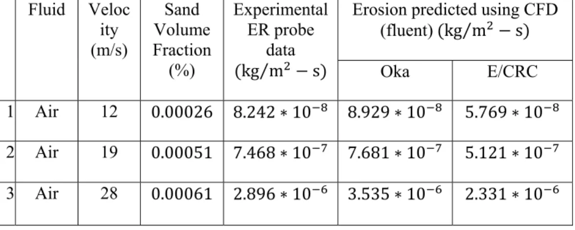
(52) 7. Results In this chapter, the average and maximum erosion rate are presented. As it was mentioned in the previous chapter, four cases (air- sand, Methane-sand, mixed gas-sand and gas- oil- sand) were investigated to obtain the average and maximum erosion rate. In all cases, the erosion estimated by using the OKA correlation and E/CRC correlation in a separate simulations with three different velocities (12m⁄s, 19m⁄s, and 28 m⁄s). Table 7-1 shows the previous experimental results on one hand and predicted erosion by using CFD model, Oka et al. and E/CRC by using FLUENT 6 [17] on the other hand. Those results were collected by using ER probe when the ER probe was placed in the middle of the outer bend of 90 degree elbow at 45 degree. But some conditions in those results (experimental and CFD based erosion) are not mentioned such a dimension of the ER probe except that the ER probe is installed in the middle of the 45 degree bend on the outer bend , and the situation of the inlet domain to know about how the particle were injected. And also the way of coupling between continuous and dispersed phases. Because of these reasons, it would be difficult to make an accurate comparison between the results in this thesis with the result in table 7-1 previous result [17]. Table 7-1 experimental and CFD predicted erosion by using Oka et al. and E/CRC models (previous work). Fluid. Veloci ty (m/s). Sand Volume Fraction (%). Experimental ER probe data (m/kg). Erosion predicted using CFD (fluent) (m/kg) Oka. E/CRC. 1. Air. 12. 0.00026. 1.2 10. 1.3 10. 8.4 10. 2. Air. 19. 0.00051 . 3.5 10 . 3.6 10 . 2.4 10 . 3. Air. 28. 0.00061 . 7.7 10 . 9.4 10 . 6.2 10 . 50.

(53) As it is shown in table 7-1, the erosion rate unit is in m⁄kg . However, the erosion rate in the STAR-CCM+ is obtained in kg⁄m s . In order to make the comparison between results in table 7-1 and the results which is obtained by the software, the result of the table 7-1 are converted from m⁄kg to kg⁄m s . The previous results can be rewritten in s as it is sown in table 7-2 shows those results. kg⁄m Table 7-2 experimental and CFD predicted erosion by using the Oka et al. and E/CRC models after converting units of erosion rate (previous work). Fluid. Veloc ity (m/s). Sand Volume Fraction (%). Experimental ER probe data kg⁄m s. Erosion predicted using CFD (fluent) kg⁄m s. 8.242 10. 8.929 10. Oka. E/CRC. 1. Air. 12. 0.00026. 2. Air. 19. 0.00051 7.468 10 7.681 10 . 5.121 10 . 3. Air. 28. 0.00061 2.896 10 3.535 10 . 2.331 10 . 5.769 10. In this thesis, in all cases the average erosion rate for the whole elbow was obtained. While, the average erosion rate was found only on the ER probe in the previous work (experimental and CFD based erosion prediction). As it was mentioned, the dimension of the ER probe is not given in the previous work. In order to make a comparison, the dimension of the ER probe was guessed to obtain the average erosion rate on the ER probe. This case was investigated only when the sand particle flows in the air flow. The dimension of the ER probe is (0.0142 * 0.0364 meter) and it is located at 4 degree above and under 45 degree line in the middle of the 90 degree. It means that in air-sand case the erosion rate was found for the whole elbow and the ER probe which the dimensions was guessed and it might be different with the ER probe used in the previous work. Figure 7-1 shows the ER probe which is installed at outer of the 90 degree elbow in this thesis.. 51.

(54) Fiigure 7-1 90 degree d elbow with w ER probe shown in the m middle of outeer bennd at 45 degreee. In this t thesis, all results obtainned under som me conditionss which some of them m mentioned and a the other conditions c willl be addressedd in this chaptter. As it was mentiooned in the prrevious chapteer, 80 515 cells were usedd to messh the 90 degrree elbow. Meeanwhile, the particles were injected in the inlett domain at 0.05 0 centimetrres at the beg ginning of thee 0.2 centimettres extrruded pipe by using part injeector. Part injeector representts a collectionn of injection point (19992 points) at the inlet dom main and the paarticle velocityy is r equaal to the veloocity of the flluid. In all caases, the averrage erosion rate obtaained for the whole w 90 degree elbow. In addition, the average erosiion rate for the ER probe was founnd only for aiir-sand case w with all velocitties (12 , 19 , and a 28 ). Bearing B in min nd, the dimenssion of ER proobe which was used in this thesis is assumed to be similar tto the ER proobe which was used originally in the previous work. And aalso the partiicle ween the prevvious works with w interrjected condittion might be different betw conddition in this thhesis. Thee 90 degree elbbow has 0.2 centimetres c pip pe on both siddes of the elboow. Thee interfaces bettween the inleet and out let of o the elbow w with the extrudded pipees in both inllet and outlet will help to transfer the iinlet and out let dom main from the beginning annd the end off the 90 degrree elbow to the begiinning and end of the extruuded pipe. Thee particles werre injected at the pressentations girdd which is creaated at the beg ginning of thee inlet pipe moore 52.

(55) precisely at 0.05 m at the beginning of the inlet domain in all cases. To be clearer, the results of the average erosion rate for the first case (airsand) for the ER probe and for whole elbow will be shown at first. After obtaining the result for ER probe, it will be compared with the previous result. Secondly, the average erosion rate results for the whole elbow in all other three cases will be shown. Finally, the tables of result for all cases with each velocity (12m⁄s, 19m⁄s, and 28 m⁄s) individually will be shown. Starting with the air-sand simulation to find the average erosion rate when the Oka model was used with the velocity of 12 m⁄s. Figure 7-2 shows the erosion rate distribution on ER probe and on the whole elbow. The average erosion rate at the ER probe and whole elbow are equal to 5.02475 10 , kg⁄m s respectively. Hoverer, the maximum and 6.92596 10 erosion rate is equal to 7.04349 10 kg⁄m s). On the other hand, the average erosion rate on the ER probe and on the whole elbow are equal to 2.64317 10 and 4.29565 10 kg⁄m s) respectively when E/CRC model was used. And the maximum erosion rate is equal to 4.03986 10 kg⁄m s). Figure 7-3 shows the erosion rate distribution by E/CRC model.. Figure 7-2 Erosion rate distribution in an elbow (Oka model, Air-Sand, ⁄ V=12 m/s, Maximum erosion rate= . .. 53.

(56) Figure 7-3 Erosion rate distribution in an elbow (E/CRC model, Air-Sand, ⁄ V=12 m/s), Maximum erosion rate= . . In the same manner, the average erosion rate on the ER probe and whole elbow were obtained by using both the Oka and E/CRC models when the velocity is set to 19 m⁄s. When the Oka model was used, the average erosion rate on the ER probe and whole elbow are equal to 1.18556 10 and 2.02115 10 kg⁄m s) respectively. Meanwhile, the maximum erosion rate is equal kg⁄m s). The erosion rate distribution in an elbow to 1.68864 10 can be seen in figure 7-4. On the other hand, the average erosion rate on the ER probe and whole elbow are equal to 2.43179 10 and 4.15307 kg⁄m s) respectively when E/CRC model was used. And the 10 maximum erosion rate is equal to 3.71072 10 kg⁄m s). Figure 7-5 shows the erosion rate distribution in an elbow.. 54.

(57) Figure 7-4 Erosion rate distribution in an elbow (Oka model, Air-Sand, ⁄ V=19 m/s, Maximum erosion rate = . .. Figure 7-5 Erosion rate distribution in an elbow (E/CRC model, Air-Sand, ⁄ V=19 m/s, Maximum erosion rate= . . Finally, the results were obtained when the velocity set to 28 m⁄s for both the Oka model and the E/CRC model. The average erosion rate on the ER probe and whole elbow are equal to 1.37818 10 and 2.34680 10 kg⁄m s) respectively with the Oka model. While the average erosion 55.

(58) rate on the ER probe and whole elbow are equal to 1.11805 10 and kg⁄m s) respectively when E/CRC model was used. 1.89333 10 Meanwhile, the maximum erosion rate is equal to 2.09792 10 with the Oka model and 1.69428 10 kg⁄m s) with E/CRC model. Figure 76 and 7-7 shows the erosion rate when the velocity is 28 m⁄s for both Oka model and E/CRC model respectively.. Figure 7-6 Erosion rate distribution in an elbow (Oka model, Air-Sand, ⁄ . V=28 m/s), Maximum erosion rate= .. 56.

(59) Figure 7-7 Erosion rate distribution in an elbow (E/CRC model, Air-Sand, ⁄ . V=28 m/s, Maximum erosion rate= . Table 7-3 shows the result for predicted average erosion rate by using STAR-CCM+ on the ER probe with both the Oka and the E/CRC model with different velocities namely 12 m⁄s, 19 m⁄s, and 28 m⁄s. Figure 7-8 and 7-9 are line and bar charts which shows the variation of average erosion rate with varying velocity on ER probe. Table 7-3 CFD predicted average erosion rate for air-sand by using the Oka et al. and the E/CRC models on ER probe. Fluid. Velocity (m/s). Sand Volume Faction (%). Average Erosion rate predicted by using CFD (STARs CCM+) kg⁄m Oka E/CRC. 1. Air. 12. 0.00026. 5.02475 10. 2.64317 10. 2. Air. 19. 0.00051 . 1.18556 10. 2.43179 10 . 3. Air. 28. 0.00061 . 1.37818 10. 1.11805 10 . 57.

(60) Figure 7-8 variation of average erosion rate with varying velocity for airsand on an ER probe.. Figure 7-9 variation of average erosion rate with varying velocity for airsand on an ER probe. Table 7-4 shows the result for predicted average erosion rate by using STAR-CCM+ on the whole elbow with both the Oka and the E/CRC model with different velocities namely 12 m⁄s, 19 m⁄s, and 28 m⁄s. Figure 7-10 58.

(61) and 7-11 shows the variation of average erosion rate with varying velocity on whole elbow. Table 7-4 CFD predicted average erosion rate for air-sand by using the Oka et al. and the E/CRC models on whole 90 degree elbow. Fluid. Veloc ity (m/s). Sand Volume Fraction (%). Average Erosion rate predicted by using CFD (STARCCM+) kg⁄m s Oka E/CRC. 1. Air. 12. 0.00026. 6.92596 10. 4.29565 10. 2. Air. 19. 0.00051 . 2.02115 10 . 4.15307 10 . 3. Air. 28. 0.00061 . 2.34680 10 . 1.89333 10 . Figure 7-10 variation of average erosion rate with varying velocity for airsand on whole elbow.. 59.

(62) Figure 7-11 variation of average erosion rate with varying velocity for air sand on whole elbow. Table 7-5 shows the result for predicted maximum erosion rate by using STAR-CCM+ on the whole elbow with both the Oka and the E/CRC model with different velocities namely 12 m⁄s, 19 m⁄s, and 28 m⁄s. These results can be seen in the figure 7-12 and 7-13 respectively. Table 7-5 CFD predicted maximum erosion rate for air-sand by using the Oka et al. and the E/CRC models on whole 90 degree elbow. Fluid. Veloc ity (m/s). Sand Volume Fraction (%). Maximum Erosion predicted by using CFD (STARCCM+) kg⁄m s Oka E/CRC. 1. Air. 12. 0.00026. 7.04349 10. 2. Air. 19. 0.00051 . 1.68864 10 3.71072 10 . 3. Air. 28. 0.00061 . 2.09792 10 1.69428 10 . 60. 4.03986 10.

(63) Figure 7-12 variation of maximum erosion rate with varying velocity for air-sand on whole elbow.. Figure 7-13 variation of maximum erosion rate with varying velocity for air-sand on whole elbow.. 61.

(64) Finally, figure 7-14 and 7-15 shows the comparison of previous result (Experimental, Oka, and E/CRC by using Fluent) with CFD predicted by using STAR-CCM+ on the ER probe and whole elbow.. Figure 7-14 comparison of previous result (Experimental, Oka, and E/CRC by using Fluent) with CFD predicted by using STAR-CCM+ on ER probe and whole elbow.. 62.

(65) Figure 7-15 comparison of previous result (Experimental, Oka, and E/CRC by using Fluent) with CFD predicted by using STAR-CCM+ on ER probe and whole elbow. Same procedure needs to be followed to show the average erosion rate with different velocities namely 12m⁄s, 19m⁄s, and 28 m⁄s for the three remaining cases (Methane, Mixed gas, and Oil-gas). But in those cases only the average and maximum erosion rate for the whole elbow will be discussed and showed since the data for those cases are not available to be compared with. In the second case, methane was used to model the continuous flow. While the average and maximum erosion was determined by implementing the same models (the Oka and E/CRC). Figure 7-16 and 7-17 shows the erosion rate distribution for the Oka and E/CRC models when the velocity was set to 12 m/s. The average erosion rate are equal to 7.09425 10 and 4.40264 10 kg⁄m s) by using Oka and E/CRC model respectively. While the maximum erosion rate by using the Oka and E/ERC models are equal to 7.89857 10 kg⁄m s) and 5.24465 10 kg⁄m s) respectively.. 63.

(66) Figure 7-16 Erosion rate distribution in an elbow (Oka model, Methane⁄ Sand, V=12 m/s, Maximum erosion rate=8.89857 .. Figure 7-17 Erosion rate distribution in an elbow (E/CRC model, Methane⁄ . Sand, V=12 m/s, Maximum erosion rate= . When velocity was set to 19 m/s, the average erosion rate are equal to 2.06742 10 and 4.25280 10 kg⁄m s) by using the Oka and E/CRC models respectively. Meanwhile, the maximum erosion rate are equal to 2.04856 10 kg⁄m s and 4.68135 10 kg⁄m s) by using the Oka and E/ERC models respectively. The erosion rate distribution 64.

(67) in an elbow for the Oka and E/CRC models can be seen in figure 7-18 and 7-19 respectively.. Figure 7-18 Erosion rate distribution in an elbow (Oka model, Methane⁄ Sand, V=19 m/s, Maximum erosion rate= . .. Figure 7-19 Erosion rate distribution in an elbow (E/CRC model, Methane⁄ Sand, V=19 m/s, Maximum erosion rate= . . 65.

(68) Finally, the erosion rate distribution on the elbow for the velocity 28 m/s can be seen in figure 7-20 and 7-21 for the Oka and E/CRC models respectively. In this case, the average erosion rate are equal to 2.39960 10 and 1.93419 10 kg⁄m s) by using the Oka and E/CRC models respectively. Meanwhile, the maximum erosion rate are equal to 2.37642 10 kg⁄m s) and 1.94470 10 kg⁄m s) by using the Oka and E/ERC models respectively.. Figure 7-20 Erosion rate distribution in an elbow (Oka model, Methane⁄ Sand, V=28 m/s, Maximum erosion rate= . .. 66.

(69) Figure 7-21 Erosion rate distribution in an elbow (E/CRC model, Methane⁄ Sand, V=28 m/s, Maximum erosion rate= . . Table 7-6 shows the average erosion rate in an elbow for all velocities and for both the Oka and E/CRC models when sand particles flow in methane. Then those results converted to a line and bar charts to show the variation of average erosion rate with varying velocity in this case. This can be seen in figure 7-22 and 7-23. Table 7-6 CFD predicted average erosion rate for methane-sand by using the Oka et al. and E/CRC models on whole 90 degree elbow. Fluid. Veloc ity (m/s). Sand Volume Fraction (%). Average Erosion rate predicted by using CFD (STARCCM+) kg⁄m s Oka E/CRC. 1. Methane. 12. 0.00026. 7.09425 10. 2. Methane. 19. 0.00051 . 2.06742 10 4.25280 10 . 3. Methane. 28. 0.00061 . 2.39960 10 1.93419 10 . 67. 4.40264 10.

(70) Figure 7-22 variation average erosion rate with varying velocity for methane-sand on whole elbow.. Figure 7-23 variation average erosion rate with varying velocity for methane-sand on whole elbow.. 68.

(71) Table 7-7 shows the maximum erosion rate in an elbow for all velocities and for both the Oka and E/CRC models when sand particles flow in methane. Then those results converted to a line and bar charts to show the variation of average erosion rate with varying velocity in this case. This can be seen in figure 7-24 and 7-25. Table 7-7 CFD predicted maximum erosion rate for methane-sand by using the Oka et al. and E/CRC models on whole 90 degree elbow. Fluid. Veloc ity (m/s). Sand Volume Fraction (%). Maximum Erosion rate predicted by using CFD (STARCCM+) kg⁄m s Oka E/CRC. 1. Methane. 12. 0.00026. 7.89857 10. 5.24465 10. 2. Methane. 19. 0.00051 . 2.04856 10 . 4.68135 10 . 3. Methane. 28. 0.00061 . 2.37642 10 . 1.94470 10 . Figure 7-24 variation of maximum erosion rate with varying velocity for 69.

(72) methane-sand on whole elbow.. Figure 7-25 variation of maximum erosion rate with varying velocity for methane-sand on whole elbow. In the third case, mixed gas (0.91 of Methane (CH4), 0.056 of Propane (C3H8), 0.016 of Nitrogen (N2), 0.013 of Butane (C4H10), 0.003 of Carbon Dioxide (CO2), and 0.002 of Hydrogen (H2)) was used to model the continuous flow. And the erosion was determined by implementing the same models (the Oka and E/CRC) as used for estimating erosion in the previous cases. At the beginning, the velocity was set to 12 m/s and by using each one of those erosion models (the Oka and E/CRC). The average erosion rate was obtained and equal to 7.05580 10 and 4.35136 10 kg⁄m s) by using the Oka and E/CRC models respectively. The maximum erosion rate by using the Oka model is equal to 7.70118 10 kg⁄m s). While it’s equal to 5.22432 10 kg⁄m s) by using E/CRC model. Figure 7-26 and 7-27 shows the erosion rate distribution in an elbow for the Oka and E/CRC models respectively.. 70.

(73) Figure 7-26 Erosion rate distribution in an elbow (Oka model, Mixed gas⁄ Sand, V=12 m/s, Maximum erosion rate= . .. Figure 7-27 Erosion rate distribution in an elbow (E/CRC model, Mixed gas-Sand, V=12 m/s, Maximum erosion rate= . ⁄ .. 71.

(74) The erosion rate distribution in an elbow for the Oka and E/CRC models when velocity is set to 19 m/s can be seen in figure 7-28 and 7-28 respectively. The average erosion rate are equal to 2.05891 10 and 4.24944 10 kg⁄m s) by using the Oka and E/CRC models respectively. Meanwhile, the maximum erosion rate are equal to 1.98286 10 kg⁄m s) and 4.40885 10 kg⁄m s) by using the Oka and E/ERC models respectively.. Figure 7-28 Erosion rate distribution in an elbow (Oka model, Mixed gas⁄ . Sand, V=19 m/s, Maximum erosion rate= .. Figure 7-29 Erosion rate distribution in an elbow (E/CRC model, Mixed gas-Sand, V=19 m/s, Maximum erosion ⁄ rate= . . 72.

(75) Finally, figure 7-30 and 7-31 shows the erosion rate distribution in an elbow at velocity equal to 28 m/s with both the Oka and E/CRC models respectively. In this case, the average erosion rate are equal to 2.38654 10 and 1.92290 10 kg⁄m s) by using the Oka and E/CRC models respectively. Meanwhile, the maximum erosion rate are equal to 2.37042 10 kg⁄m s) and 1.85034 10 kg⁄m s) by using the Oka and E/ERC models respectively.. Figure 7-30 Erosion rate distribution in an elbow (Oka model, Mixed gas⁄ . Sand, V=28 m/s, Maximum erosion rate= .. Figure 7-31 Erosion rate distribution in an elbow (E/CRC model, Mixed gas-Sand, V=28 m/s, Maximum erosion ⁄ rate= . . 73.

No results found