THERMAL STORAGE SOLUTIONS FOR
A BUILDING IN A 4
TH
GENERATION
DISTRICT HEATING SYSTEM
Development of a dynamic building model in Modelica
ANDERSSON PONTUS
ERIKSSON RICKARD
ABSTRACT
The world is constantly striving towards a more sustainable living, where every part of contribution is greatly appreciated. When it comes to heating of buildings, district heating is often the main source of heat. During specific times, peak demands are created by the tenants who are demanding a lot of heat at the same time. This demand peak puts a high load on the piping system as well as the need for certain peak boilers that run on non-environmental friendly peak fuel. One solution that is presented in this degree project that solves the time difference between production and demand is by utilizing thermal storage solutions. A dynamic district heated building model is developed with proper heat propagation in the pipelines, thermal inertia in the building and heat losses through the walls of the building. This is all done utilizing 4th generation district heating temperatures. Modelica is the tool that
was used to simulate different scenarios, where the preheating of indoor temperature is done to mitigate the possibility for demand peaks. Using an already existing model, implementation and adjustments are done to simulate thermal storage and investigate its effectiveness in a 4th generation district heating system. The results show that short-term
energy storage is a viable solution in concrete buildings due to high building mass. However, combining both 4th generation district heating with storage in thermal mass is shown not to
be suitable due to low temperatures of supply water, which is not able to increase the temperature of the building’s mass enough.
Keywords: Thermal storage, 4th generation district heating system, dynamic simulation,
PREFACE
This degree project in Master of Science in energy systems has been carried out at Mälardalens University. We would like to thank our supervisor Nathan Zimmerman (Mälardalen University) for supporting this degree project. During the project, he has provided us with ideas, data and interesting discussion, which lead the project forward. The project has aimed to create a model using Modelica, which simulates thermal mass storage and heat propagation in a building using 4th generation district heating system
temperatures. We hope that this can be useful to people interested in the future of district heating systems and further insight into the possibilities and solutions of thermal storage.
Pontus Andersson, Rickard Eriksson
Västerås, Sweden 2018-06-11
SAMMANFATTNING
Samhället idag strävar mot en mer hållbar framtid, för att uppnå detta utvecklas teknologier för att minska användningen av fossila bränslen och på grund av det minska utsläpp som påverkar klimatet. Ett sätt att minska användningen av fossila bränslen är att kombinera el- och värmeproduktion, med hjälp av så kallade kraftvärmeverk. Eftersom värmen används i fjärrvärmesystem så kan det hända att efterfrågan av värmeenergi under vissa tidsperioder är väldigt hög, detta kallas för värmetoppar. Kraftvärmeverken måste då kompensera för att uppnå den tillfälliga efterfrågan. Vilket leder till att en hög belastning på både system och produktionsenhet skapas. För att uppnå dessa värmetoppar på kort tid används ofta extra värmepannor som ofta drivs med olja.
Syftet med examensarbetet är undersöka hur värmelagring i ett 4:e generationens fjärrvärmesystem kan påverka en byggnads värmebehov. Detta görs genom att utveckla en byggnadsmodell som har verkliga förluster och tröghet i värmflöden.
En dynamisk modell har utvecklats i Modelica där en byggnads värmeflöden har beräknats. Fjärrvärmesystemet har dynamiska egenskaper vilket gör att värmeförluster och tidsfördröjning har beräknats hur det ser ut i verkligheten. Simuleringen är gjord med 4:e generationens fjällvärmetemperaturer. När det kommer till validering så har mätdata från Mälarenergis nät har använts för att validera fjärrvärmerören. Medan validering av byggnaden har gjorts med data samlad från litteratur. Valideringarna visar att resultat från rörmodellen motsvarar uppmäta värden och byggnadens förluster motsvarar liknande storlek på hus.
Resultaten visar att värmelagring i byggnader kan användas för att förskjuta generation av värme vid kraftvärmeverk. Däremot visas det att kombinationen av värmelagring och 4:e generationens fjärrvärmesystem inte är en lämplig lösning då temperaturer på levererat vatten inte är tillräckligt hög. En för låg temperatur på vattnet ger en temperaturhöjning hos byggnaden som in är tillräckligt snabb. Vilket leder till att byggnadens värmeförluster är högre än tillförd värme. Då slutsatsen dragits att temperaturen på levererat vatten är orsaken till en för låg tillförd värme, kan därför användningen av värmelagring därför vara mer passande där ett 3:e generationens fjärrvärmenät används.
Nyckelord: Värmelagring, 4:e generationens fjärrvärmesystem, dynamisk simulering,
TABLE OF CONTENT
1 INTRODUCTION ... 1
1.1 Background ... 1
1.1.1 Peak-creating demands ... 2
1.1.2 Thermal energy storage ... 2
1.1.3 Different generations of district heating systems ... 3
1.1.4 Description of the base model ... 3
1.2 Purpose ... 4
1.3 Research questions ... 5
1.4 Delimitation ... 5
2 LITERATURE STUDY ... 6
2.1 Peak Shaving ... 6
2.2 Peak fuels and their impact ... 6
2.3 Thermal storage technologies ... 8
2.3.1 Thermal storage in building mass ... 9
2.4 Advantages with 4th generation district heating system ... 10
2.5 Thermal dynamics ... 10
2.6 Indoor comfort level ... 11
3 METHOD ... 12
3.1 Analysis of the base model ... 12
3.2 Literature review ... 12
3.3 Choice of storage solution ... 13
3.4 Model development ... 13
3.5 Validation of model ... 13
3.6 Simulation and evaluation ... 13
4 MODELICA LIBRARY DEVELOPMENT ... 14
4.1 Plant heat exchanger ... 14
4.2.1 Pressure ... 16
4.2.2 Temperature ... 17
4.3 Mixer and Splitter ... 18
4.4 Pump ... 19
4.5 Building component ... 19
4.5.1 Heat demand ... 20
4.5.2 Thermal transmittance in building ... 20
4.5.2.1. Wall ... 21
4.5.2.2. Ceiling and floor ... 22
4.5.3 Radiator ... 23
4.6 Validation of model components ... 24
4.6.1 Validation of the district heating pipelines ... 24
4.6.2 Validation of the building ... 24
5 RESULTS ... 26
5.1 Building temperature dynamics ... 26
5.2 Radiator emission and building losses ... 32
5.3 Supply temperature delay ... 33
6 DISCUSSION ... 34 6.1 Method evaluation ... 34 6.2 Validation ... 35 6.3 Model limitations ... 35 6.4 Results discussion ... 36 6.4.1 Building temperature ... 36 6.4.2 Pipe behavior ... 37
APPENDIX 1 – THERMAL STORAGE TECHNOLOGIES
APPENDIX – DIMENSIONS AND PROPERTIES OF COMPONENTS APPENDIX 3 – DISTRICT HEATING DEVELOPMENT
APPENDIX 4 - INPUT DATA
LIST OF FIGURES
Figure 1 - Background - Base model ... 4
Figure 2 - Literature study - CHP load duration curve ... 7
Figure 3 - Method - Method scheme ... 12
Figure 4 - Modelica library development - System figure ... 14
Figure 5 - Modelica library development - Heat exchanger ... 15
Figure 6 - Modelica library development - Pipe dimension definitions ... 15
Figure 7 - Modelica library development - Building dimensions ... 19
Figure 8 - Modelica library development - Wall cross section ... 21
Figure 9 - Modelica library development - Floor and ceiling cross section ... 22
Figure 10 - Modelica library development - Validation of district heating pipes ...24
Figure 11 - Results - Case 1 original walls ...26
Figure 12 - Results - Case 1 thicker walls ... 27
Figure 13 - Results - Case 2 original walls ... 28
Figure 14 - Results - Case 2 thicker walls ...29
Figure 15 - Results - Case 3 original walls ... 30
Figure 16 - Results - Case 3 thicker walls ... 31
Figure 17 - Results - Radiator heating and building losses ... 32
Figure 18 - Results - Pipe supply temperature ... 33
LIST OF TABLES
Table 1 - Literature study - Current fuel consumption for district heating ... 7Table 2 - Literature study - Storage technology summary ... 8
Table 3 - Modelica Library Development - General HE data ... 20
NOMENCLATURE
Symbol Description Unit
K Heat emission coefficient W∙K-1
C Heat capacity W∙K-1
U Thermal transmittance W∙(m2, K)-1
α Convective heat transfer coefficient W∙(m2, K)-1
h Mixed heat transfer coefficient W∙(m2, K)-1
Stefan-Boltzmann constant W∙(m1, K4)-1
Conductive heat transfer coefficient W∙(m1, K)-1
q Heat W
Dynamic viscosity Pa∙s-1
A Area m2 v Velocity m∙s-1 Surface roughness m d Diameter m L Length m Mass flow kg∙s-1 Density kg∙m-3 Cp Heat capacity J∙(kg, K)-1
Time constant Hours
P Pressure Bar, Pa
T Temperature °C, Kelvin
f Darcy friction factor -
Re Reynolds number -
Emissivity -
Nu Nusselt’s number -
r Pressure ratio -
Pr Prandtl’s number -
ABBREVIATIONS
Abbreviation Description
CHP Combined Heat and Power
LTDH Low-Temperature District Heating
BHES Borehole Energy Storage
TES Thermal Energy Storage
RB Residential Building
OB Office Building
DHN District Heating Network
1 INTRODUCTION
To be able to mitigate the world’s impact on the climate and environment, different energy saving and emission reduction solutions is necessary. Research on both existing and new technologies to minimize the use of fossil fuels is being done to mitigate the emissions of greenhouse gases. A way of reducing fuel consumption is to utilize the heat and electricity generated in a combined heat and power (CHP) plant. The plant heats steam with a boiler, the steam then expands in a turbine, which generates electricity. Then by passing the steam through a condenser, district heating water is heated, which then is supplied to the
customers.
District heating is a technology where a grid of pipes is used to transfer heated water between different buildings. The network often consists of several circuits, where heat exchangers (HE) is used for transfer of heat between primary and secondary line. The generation of the heat is often combined with the generation of electricity by the use of a CHP, as previously mentioned. In Sweden today approximately 50% of the heat demand is covered by district heating according to Euroheat.org (2017).
The current district heating system operates at supply and return temperatures of around 100°C/50°C stated in Lund et al. (2014). The next generation (4th generation) of district
heating will operate with temperatures around 50°C/20°C. This reduces the system losses and will increase the number of heat sources that can supply heat to the district heating network (DHN).
1.1 Background
By having many buildings connected to the same grid the heat demand occasionally experience peaks loads due to recipients using hot water at the same time, for example during mornings. This also causes a peak in the generation, and the maximum load of the CHP plant needs to be high enough to supply heat to cover the heat demand. Looking at the Västerås-region in Sweden, this is important as it is shown that approximately 98% of the city buildings are connected to the district heating network, which is supplied by Mälarenergi. (Mälarenergi.se, 2018b).
1.1.1 Peak-creating demands
The heat demand for a building is dependent on the customer’s usage of heat as well as outside temperature. The temperature level inside the building needs to be within the comfort level of the tenants. The seasonal heat demand is highest during the winter, end of November until the middle of March as seen in the article by Gadd & Werner (2013). This is due to low outdoor temperature, which increases the heat demand in residential and non-residential buildings. However, the heat demand peaks do not only exist in the seasonal perspective but can also be seen in a daily view. The peaks are at their highest at 6-8 in the morning when people are starting their day, which is shown in an article written by Gadd & Werner (2013). To be able to cover these peaks the dimension of the grid must be designed for the maximum demand so that enough heat can be distributed during the peak hours. The problem with these heat demand peaks is that the CHP plant needs to compensate for these sudden increases in demand, from low usage during the night to high usage in the morning, from a mild winter day to a cold winter day. To compensate for the high peaks during the winter season the company that supplies the heat is sometimes forced to use a backup boiler. The backup boiler often runs on expensive peak load fuels. Commonly used fuel is oil, which is used in oil burners to generate heat to the district heating system. These fuels are not only expensive but also not environmentally friendly and not a sustainable way of supplying heat in the long terms (Vattenfall.com, 2013).
The building structure is one of the many important aspects when it comes to heating of buildings. Karlsson (2012a) mentions that the time constant difference between a heavy (well insulated) and a light (poor insolated) building could be up to three times. That means that the heavy building heats up or cools down three times slower than the light building. The author explains that it is because a light building reacts much faster to outdoor temperature changes, which is going to impact heat demand spikes.
1.1.2 Thermal energy storage
A way to mitigate the demand peaks is to use a technology called thermal energy storage. It is a technology that is used to store energy in different kind of elements. By implementing thermal storage in the district heating system, the stability and heat-safety could be increased. This is done by storing hot district heating during hours with low demand and then used to supplement the district heating grid so that production peaks may be reduced according to Tveit, Savola, Gebremedhin, & Fogelholm (2009).
Previous research has been done both within the thermal storage and the low-temperature district heating field, but only a handful of articles have been done by combining them both. Verda & Colella (2011) investigates the energy savings with a thermal storage tank in the district heating system. The paper shows that energy saving can be obtained by producing heat at night and using it during the day.
An article by Lund et al. (2014) has researched the advantages of adapting to a 4th generation
district heating system with lower temperature. The study shows the flexibility and the energy saving that could be utilized by using renewable low-temperature heat sources.
In the research paper by Dominković, Gianniou, Münster, Heller, & Rode (2018), the authors study the possibility of storing heat in the building’s mass. This is investigated using a linear optimization model, where different types of preheating periods are investigated. The article also sets up the model to minimize the total cost of the system.
1.1.3 Different generations of district heating systems
When development reached the so-called 3rd generation of district heating, a lot of the
characteristics in the distribution network were changed. Generally, lower temperatures below 100˚C were used (Lauenburg, 2014). This allowed cheaper components in the system such as piping. Distribution pipes used in third generation district heating are plastic jacket pipes (Frederikson & Werner, 2013).
As of today, there is currently no specific definition of the 4th generation district heating. As
previous generations have been developed into using lower temperature water, which has enabled the system to use cheaper materials for piping (Lauenburg, 2014). Continued development in the same direction can be seen as useful, as it provides a way of utilizing new heat sources for the production of hot water. These sources, such as waste heat from industrial processes and renewable sources can, therefore, be utilized as heat for the DHN. By implementing renewable sources as a heat source, a significant decrease in fuel consumption can be achieved. It is said that operating temperatures in 4th generation district heating may
vary within the range 30-70˚C (Lund et al., 2014). Cheaper investment cost can, therefore, be reached as using lower temperatures allows cheaper materials to be used (Frederikson & Werner, 2013). Earlier generations of district heating systems can be found in APPENDIX 3. Installing thermal storage with low-temperature district heating system is a way of combining both technologies. The benefits of this system are that it brings flexibility to the thermal storage since temperature water can be generated from multiple low-temperature sources (Lund et al., 2014). Thermal storage brings heat security as well as peak shaving opportunities to reduce peak load demands and the low-temperature district heating lowers the pipe losses (Verda & Colella, 2011).
1.1.4 Description of the base model
The base model that this degree project will continue and develop was developed in OpenModelica in a degree project performed by Kamal (2017). The model is designed to simulate a simplified fictitious case of a city area in Västerås using 4th generation district
heating temperatures and is built to simulate the case in steady-state. The model simulates a case of 30 buildings and they can be divided into two groups, residential buildings (RB) and
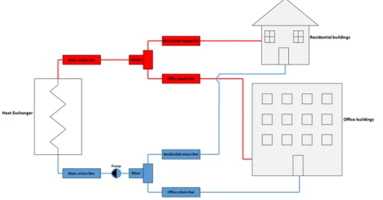
The case simulated is located in Kungsängen, Västerås Sweden and an illustration of the model is shown in Figure 1.
Figure 1 - Background - Base model
The model contains an HE, where supply heat from Mälarenergi’s CHP plant is used as heat source. Heat from the hot side of the HE is transferred to the cold side. The heated water on the cold side is then transported through supply piping out in the district heating grid. In the network, a splitter is used to divide the mass flow between the RB and the OB. The buildings use a simplified demand model, where measured demand for one house was supplied by Mälarenergi. The model uses the demand for one home and a factor of 15 to multiply it to simulate a case of 15 houses for each category. After heat exchange in the buildings has occurred, cold water returns to a mixer, where the flows from each building category are mixed into one stream. The water is then transported to the HE through return pipes. The pipe components in the model are used to take temperature losses during transportation into consideration.
1.2 Purpose
The purpose of this degree project is to investigate the effectiveness of thermal storage in a 4th
generation district heating system. An existing model of a fictitious case in Västerås, Sweden is used as a base. Improvements are made by implementing thermal storage to the building to evaluate its impact on the demand. Furthermore, the study also aims to adjust aspects in the base model to be able to simulate a dynamic case that replicates real-life heat propagation and heat losses. The buildings characteristics and thermal capacity are developed to simulate accurate thermal inertia in walls, ceiling and floor.
1.3 Research questions
As heat production peaks have substantial stress on both the plant and distribution grid, potential improvement exists by reducing these peaks that occur during specific times. Implementation of a thermal storage solution is investigated to mitigate the building’s heat demand pattern. Therefore the research questions of the degree project are:
How can thermal energy storage affect a residential buildings heat demand?
What is the compatibility between a 4th generation district heating system and short-term
energy storage?
1.4 Delimitation
The degree project was a continuation of an existing model, where the location of the simulated case was limited to the area of Västerås. Weather data and measured district heating temperatures for the simulation are limited to data from the year 2016. No major changes in the grid layout of the model have been done from the base model.
The building dimensions are simplified by using same length of the walls, where walls, floor and ceiling are exposed to external heat fluctuations. The floor is adjacent to the soil and the other walls of the building are exposed to the outdoor air. The building does not take into account any ventilation, exchange of air, human activity or furniture. The walls are assumed to be covered by concrete, where no windows are taken into consideration.
2 LITERATURE STUDY
The literature study was performed using scientific articles with peer-reviewed priority, where several areas were related do district heating has been reviewed. To be able to structure the model and its behavior theories and data from previous work has been used, studied areas are peak shaving, thermal storage technologies, peak load fuels, 4th generation
district heating, thermal dynamics of buildings and pipes and thermal comfort levels of buildings. The literature study will bring methods and data on how to develop the thermal
storage model.
2.1 Peak Shaving
A so-called peak is created when customers have a significantly larger demand in comparison to the average load demand. This is applied to both thermal and electric needs. Production units must be designed to cover the highest demand-peaks so that enough energy can be supplied at all times (ABB.com, 2018). As the dimensions of the production plants and distribution grid are designed for the maximum demand, it means that the total capacity is not always utilized. This leads to reduced profitability for the responsible distributor as a high investment cost is required. An increased fee for customers is often done to cover the financial losses that occur due to this consequence (Kein Huat Chua, Yung Seng, & Morris, 2016).
Combined heat & power plants may not always be enough to cover the sudden peaks, a solution to this problem is to implement a backup steam boiler that is utilized during the peak hours. However, steam boilers that are used for this purpose may use fuels that are not beneficial for the environment (Vattenfall.com, 2013). To reduce the use of fossil fuels, peak shaving solutions needs to be investigated. Peak shaving methods not only reduce the usage of fossil fuel usage but may also lead to a reduced investment cost as dimensioning of heat sources and distribution grids can be installed for smaller maximum capacity (Frederikson & Werner, 2013).
2.2 Peak fuels and their impact
Supplying a district heating grid with enough heat to cover the load is often solved by using more than one heat generating unit. A common solution is to use three different heat production units for the generation of heat. A CHP plant, electric boiler and a fuel boiler are the main units that are used. The CHP unit is used to cover the base load throughout a year while the fuel boiler is only used during peak hours. The electric boiler acts as a backup for warm periods, where the demand is low, the CHP plant is non-operational and electricity prices are low (Frederikson & Werner, 2013). An example of a load duration curve is displayed in Figure 2, reprinted from (Flores, Lacarrière, Chiu, & Martin, 2017).
Figure 2 - Literature study - CHP load duration curve
Mälarenergi in Västerås use a similar solution, where the mixture used in different boilers is shown in Table 1. Renewable fuels are wood chips, secondary wood fuels and flue gas condensation. Peat is peat briquettes. Recycled fuels are household waste and industrial waste. Fossil is coal, Heating Oil 1 (E01) and Heating Oil 5 (E05) (Mälarenergi.se, 2016). Ever since 2014, the fossil fuel usage has been decreasing and the recycled fuels have been increasing. This is because Mälarenergi installed a new burner (Burner 6) that uses recycled fuels to generates electricity and heat, where the fuel consumption is displayed in Table 1 (Mälarenergi.se, 2018a).
Table 1 - Literature study - Current fuel consumption for district heating
Year 2012 2013 2014 2015 2016 2017
Renewables [%] 47,2 46,6 45,9 49,0 55,1 55,1
Peat [%] 27,1 5,6 3,0 4,0 3,2 3,2
Recycled fuels [%] 0,0 0,0 28,3 38,0 35,7 35,7
Fossil [%] 25,7 47,8 22,8 9,0 6,0 6,0
The fossil fuels Mälarenergi uses for their burners are “Heating Oil 1”, “Heating Oil 5” and coal, where heating oil 1 is used for smaller scale heating such as residential heating and heating oil 5 is used in larger heating plants. Both of the heating oil’s emit Nitrogen, Sulphur and trace metals when combusted and coal emits carbon dioxide (SPBI.se, 2010).
2.3 Thermal storage technologies
Thermal energy storage (TES) is a technology that is used to store energy in different forms. By utilizing various heat sources and combinations of technology, multiple ways of storing heat is made possible. According to Nuytten, Claessens, Paredis, Van Bael, & Six (2013) one of the main differences in their application is that the energy can either be stored in the short-term or long-term storage. Both of the technologies have the potential to mitigate the heat demand. Below in Table 2, a summary of pros and cons are listed by each storage technology. A more detailed summary of the technologies is presented in APPENDIX 1.
Table 2 - Literature study - Storage technology summary
Storage technologies: How it works: Pros: Cons:
Thermal mass storage Preheating of buildings is utilized to store energy in the mass of the building. The thermal inertia of the building mitigates the demand peaks. Cheap due to no investment cost Only short‐term storage Thermal storage tank Hot water is stored in a tank/container. Injecting hot water to mitigate demand peaks. Short and long‐term storage Can be installed underground Cheap storage medium Expensive due to tank investment Borehole thermal energy storage Hot water is circulated through pipes in the ground. Utilizes the geothermal energy to recover heat. Short and long‐term storage Can be installed underground Cheap storage medium Expensive investment cost Latent storage Stores energy in a phase changing material. By altering the phase of the material, energy can be charged/discharged. High storage capacity per volume High performance Expensive due to material cost Chemical storage Utilizes chemical bonds to store energy, chemicals that have a reversible process. By reversing the process heat can be charged/released. High storage capacity per volume Low losses Expensive due to chemical cost
2.3.1 Thermal storage in building mass
A way of utilizing the mass of the building as thermal storage is mentioned in the article by Kensby, Trüschel, & Dalenbäck (2015a). By using the thermal inertia in a building with good insolation, over and under heating a building makes a way of storing thermal energy. The space heating comfort zone is an important aspect since the tenants do not want too hot or too cold indoor temperature. The temperature difference outside the comfort zone is said to be approximately 1-2°C stated in the article by Romanchenko, Kensby, Odenberger, & Johnsson (2018). The thermal mass storage can only be used within a short timeframe since the mass of the building cannot store heat very long. Hence, the focus lies to reduce the short-term peak loads caused in mornings and evenings (Olsson Ingvarson & Werner, 2008). The thermal mass storage works by building up thermal inertia in the mass of the building. This is done by raising the indoor temperature 1-2°C above the set temperature. The heat is then stored in the building mass such as in the walls, floor and ceiling. The pre-heating is of the building is done when the demand is low, which mitigates the demand variations and acts as a heat buffer to cover demand peaks that occur in mornings (Romanchenko et al., 2018). A study performed by Kensby (2015) shows a pilot test that certain types of buildings are more feasible to use as thermal storage. The pilot test consists of two types of structures: light & heavy. The difference between the two types of structures is the thermal mass in the buildings. A building classified as a light building typically has a core of wood or steel. A building of the heavy type has a core of concrete. As the buildings have different cores, it results in various capacities in heat storage. The article shows that a heavy building can handle large variations of heat deliveries while still maintaining a comfortable indoor climate.
It is shown that by implementing about 500 substations of short-term TES in large RB is approximately equivalent to installing a hot water storage tank with a volume of 14,200 m3 in
Gothenburg. Using short-term TES like this is calculated to reduce the start/stop of heat generation units to minimize the use of oil and gas by 10-20% (Kensby, 2015).
In the article by Kossak & Stadler (2015) the authors develop a model for room temperature prediction using the building storage mass as a component. This is done by defining every heat flow inside the building and accurately calculate the energy losses. Then the mass of the building acts as an insulator and storage of heat.
2.4 Advantages with 4
thgeneration district heating system
The low-temperature district heating makes it possible to utilize alternative heat sources for district heating production. This makes it feasible to use renewable energy sources as heating source in the 4th generation district heating system (Nuytten et al., 2013). Different energy
sources could be according to the article by Fang, Xia, Zhu, Su, & Jiang (2013) solar heat from solar panels, geothermal heat from the ground and industrial waste heat. The usage of renewable energy sources decreases the usage of fossil fuels that could have been used to heat district heating water. The author’s show that the alternative heat sources also give flexibility to the system, since the source of heat can be accessed from multiple low-temperature sources.
The main difference between the 3rd generation district heating and the 4th generation district
heating system is the temperatures. The 3rd generation DHN has a supply temperature of
90-100°C and return temperature of 40-50°C, where the low temperatures of 40-50°C in the supply pipe and roughly 20°C in the return pipe in a 4th generation DHN (Lund et al., 2014).
Lund et al. (2014) state that the pipe dimensions can be reduced in the low-temperature district heating (LTDH). Smaller pipes make it possible to use twin pipes that results in a lower heat loss than current single 3rd generation pipes. The heat loss in the low-temperature
pipes is reduced because of the very low or non-existent heat exchange between the supply and return pipe.
The article Persson & Renström (2013) discusses and evaluates the advantages that can be utilized by using the LTDH for appliances in the households. The dishwasher and laundry machine are examples of appliances that can run on low-temperature district heating water. The study shows that the energy reduction by using this method can reduce the energy usage by the machines by roughly 50%.
2.5 Thermal dynamics
The thermal dynamics of the building is an important aspect since it controls the behavior of the building’s heat flows. The walls of the building protect the inner air temperature from major fluctuations (Ozel, 2014). Therefore the wall characteristics and dynamics will create a time difference in temperature change depending on the materials inside the wall. The article by Luo, Zhu, Lim, & Huang (2018) simulates a building strategy based on the first law of thermodynamics. By defining the total energy that is exchanged between the different thermal zones the temperature within the wall is calculated. The equations in the various thermal zones are dependent on time and temperature, which makes it dynamic, creating the temperature and time difference.
The insulation and material of the building’s envelop play a big role when it comes to the temperature changes. Reynders, Baetens, & Saelens (Glenn Reynders, Baetens, & Saelens, 2012) presents that the thickness of the walls, materials within the wall and heat transmission coefficient are important aspects to accurately model a building’s thermal properties. This is done to maintain a comfortable indoor temperature for the tenants.
The pipelines temperature dynamics in a district heating system is important since it will determine the delay of the supply and return temperature of the hot water. In the article by Van der Heijde et al. (2017), the experiment displays the different computation strategies when it comes to dynamic district heating pipelines. The heat loss calculations are done by a combination of the energy and continuity equation. Darcy-Weisbach friction coefficient is used in the formula to calculate the heat losses in pipes accurately.
Another way of calculating the heat losses in district heating pipelines is presented in the article Perpar, Rek, Bajric, & Zun (2012). The authors explore the possibility to determine the thermal conductivity coefficient as accurate as possible. This is because a change in the thermal conductivity coefficient by 0.8 W/m,K to 1.2 W/m,K could mean an increase in total heat losses by 9% on a 116km pipe.
2.6 Indoor comfort level
The thermal comfort level is the indoor temperature that is within the comfort level of the tenants. The study by Cui, Cao, Park, Ouyang, & Zhu (2013) shows that temperatures above 26°C is higher than neutral and temperatures below 22°C is slightly cold. They concluded that too high temperatures effects both motivation and performance of the tenants.
The comfort level in the article by Kim (2013) is displaying the comfort range to be from 20-24°C. Another article by Le Dréau & Heiselberg (2016) is using 22°C as their set-point temperature and have a temperature span of 2°C.
3 METHOD
The methodology of the degree project is divided into several parts, analysis of the current model, literature review, choice of storage solution, model development and validation & evaluation. The analysis of the current model has been done by simulating and analyzing the results. Reviewing code and equations has been performed to determine the reliability of the current model. The literature review has been carried out mainly by searching for scientific articles in different databases, where ScienceDirect, Google Scholar and DiVA have been used. The development of the model and the construction of new components is carried out in the simulation program OpenModelica. Validation of the components is done by comparing measured values to simulated values or compared to values from literature. Several cases are done during the simulation, where results from each case are reviewed and evaluated. An overview of the methodology of the degree project is illustrated in Figure 3.
Figure 3 - Method - Method scheme
3.1 Analysis of the base model
As the degree project was a development of an existing model simulating a DHN. The components need to be built in a similar structure to the previously developed model. Therefore, an analysis of the current library has been done so that same structure of components can be followed. Thus, further development of the library or specific components is more straightforward. If a specific structure is followed, certain guidelines for code-writing can be made for easier development in the future.
3.2 Literature review
A literature study was performed to analyze what has been done within the field of research and to find helpful methods that could be of use for the project. The literature study has been carried out by reading scientific articles, journals and books. In the literature study, different methods for thermal storage are reviewed to find a motivation for chosen storage technology. 4th generation district heating was also examined to analyze appliance of thermal storage. Articles with other peak shaving possibilities have been investigated are also being taken into consideration during this process. Scientific articles with peer-review have been prioritized because of their objectiveness, scientific level and trust factor.
Analysis of the current model Literature review Choice of storage solution Development of new components Validation of components Simulation and evaluation
3.3 Choice of storage solution
As the literature study states, several options for thermal storage are investigated. In the model that has been developed as a part of this degree project, only one technical solution for storage was chosen for simulation. As the majority of solutions would require an investment cost of some sort, i.e. new material in existing buildings, a large tank or container. One way of utilizing thermal storage without an investment cost, is by using the already existing building as thermal storage. Therefore, this is the investigated technology in this degree project. When using this technology, control of indoor temperature is of great importance to accomplish a comfortable indoor climate for the tenants.
3.4 Model development
Model development was performed by developing previously existing model into a dynamic one. The majority of components have been rebuilt as their original code simulated a steady-state. Pressure parameters were implemented into the simulation to take velocities of heated water into consideration. Information gathered in the literature review was used during the development such as material properties and equations. Application of thermal storage in building mass that utilizes the thermal inertia was implemented during the development. This was done by implementing heat losses through building mass and heat supplied from radiators placed inside the building.
3.5 Validation of model
Measured data and literature were used to verify the behavior of the model’s components. As measured data from a 3rd generation DHN was used, several model parameters are adjusted
before the validation. Key parameters that are modified are pipe parameters and properties such as heat coefficients dependent on the pipes material and its dimensions.
Building validation was performed by calculating the building’s time constant and consulting literature to determine whether the building’s thermal dynamics are valid.
3.6 Simulation and evaluation
4 MODELICA LIBRARY DEVELOPMENT
As an improvement and continued development of the existing model and library was needed, several changes have been carried out. The main changes consist of rebuilding components to be able to simulate dynamic cases, where time is taken into consideration during the simulation. The pressure was added as a working parameter throughout the model as it has an impact on the heated water in the grid.
The model intends to use the building’s mass as storage described in 2.3.1. Therefore, the building component of the library has been updated to take heat and temperature levels into consideration. The building model is developed by adding dynamic heat equations and multiple insulation materials in walls, ceiling and floor. As Dymola was the chosen tool of simulation, all components are connected by connectors. The connectors were used to send parameters between different components. The parameters handled by the connectors is
temperature, pressure and mass flow. An overview of components in the DHN is displayed
in Figure 4.
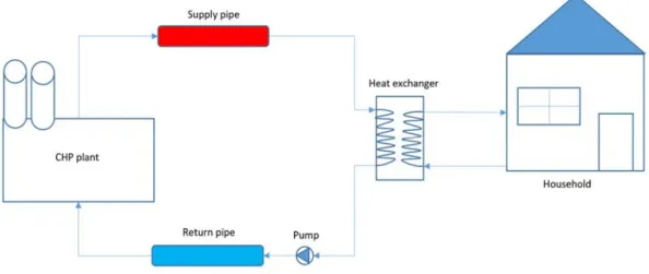
Figure 4 - Modelica library development - System figure
4.1 Plant heat exchanger
A HE located at the CHP plant is used to determine how much energy that is required to supply the building demands. As required heat generation is the interesting variable in the calculation, only the cold side of the HE is investigated. The HE is assumed to have no losses during the heat exchange which leads to the basic equation (4) to be used:
∙ ∙ (4)
Where qgen represents the total amount of energy that is required to be generated to supply
the current demand of the DHN, is the mass flow of the DHN, Tout is the temperature of the
water leaving the HE and Tin is the temperature of the water which is entering the HE from
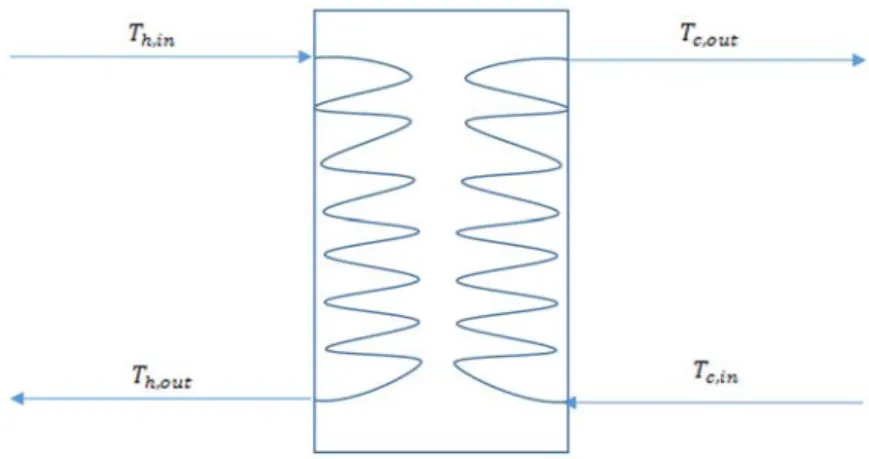
the return pipe. The layout of the inlet and outlet temperatures in the HE is shown in Figure 5.
Figure 5 - Modelica library development - Heat exchanger
The heat exchanger is used to control the charging of the building as well, this is done by increasing the load during loading periods by increasing the outlet temperature of the water. The charging occurs during night hours between 22.00-06.00 when usage of heat in a building is generally low.
4.2 District heating pipes
The distance between the CHP plant and the customer plays a significant role when it comes to heat delivery. This is because several losses in the pipeline are taken into consideration in the simulation of the model. By using dynamic components, the model takes into account how much time that is required for a particular parameter i.e. temperature, to be transported from point A to point B. Therefore, a dynamic model allows the CHP plant to predict and generate heat in time so that it can be supplied to the customer in time. Figure 6 illustrates the definitions of the pipe model.
4.2.1 Pressure
Transportation of heated water takes place during the simulation, where several losses have been taken into consideration. To determine pressure differences in pipes, Darcy-Weisbach method has been used as seen in equation (5) (P. Li et al., 2015).
∙ ∙ ∙
2 ∙ (5)
Where Ploss is the calculated pressure losses through the entire length of a pipe, is the
density of water inside the pipe, is the velocity of the water, f is the friction factor, L is the length and Di is the inside diameter of the pipe.
The velocity used in equation (5) can be expressed according to equation (6).
∙ (6)
Where Ax is the cross-sectional area of the flowing water. To calculate the cross-sectional area
equation (7) is used.
∙
4 (7)
To calculate the friction factor shown in equation (8), which is used to determine the loss of pressure over the pipe, the type of flow has to be taken into consideration. Many of the equations that are used in pressure calculations work for either laminar or turbulent flow. This is a problem as the model is intended to be functional over several seasons, where the difference in heat demand from customers may be highly variated. The mass flow of the district heating water may, therefore, be both high and low depending on what season it is. This mass flow indirectly determines whether the flow will be laminar or turbulent. Using Churchill equation from 1977 mentioned by Ghanbari, Farshad, & Rieke (2011). One method can be used to cover any flow as it is claimed that this method can be used for any Reynolds number.
8 ∙ 8 1 . (8)
Where A and B can be described as following equations (9) and (10). 2.457 ∙ ln 7 . 0.27 ∙ (9) 37530 (10)
ε is the constant of roughness dependent on the material of the pipe and the Reynolds number is calculated according to equation (11).
∙ ∙
(11)
4.2.2 Temperature
The base model has taken heat losses from transportation in pipes into consideration. However, the equations used are fitted for steady-state simulation and shown in equation (11) and (12).
∙
∙ (12)
∙ ∙ (13)
To make the model simulate a dynamic case the equation of temperature loss was replaced by a method that uses a node system to visualize the heat propagation throughout the pipe. The method first calculates the inlet and outlet temperatures of the pipe and water, where equation (14) calculates the pipe wall temperature and equation (15) calculates the water temperature. The node placement in the equations is represented by the variable i.
∙ 4 ∙ ∙ ∆ ∙ ∙ ∙ ∆ ∙ ∙ ∙ (14) ∙ ∙ ∙ ∆ ∙ ∙ ∙ 4 ∙ ∙ ∆ ∙ ∙ ∆ (15)
As in- and outlet temperatures are calculated the temperature distribution within the pipe was calculated according to equation (16).
∙ ∙ ∙ ∆ ∙ ∙ ∗ 4 ∙ ∙ ∆ ∙ ∙ 2 ∙ ∆ ∙ 2 ∙ 2 ∙ ∆ (16)
To determine the temperature of the pipe wall, thermal transmittance (U) between the pipe wall and insulation was calculated according to equation (17).
1 ∙ ln 2 ∙ ∙ ln 2 ∙ (17)
Where Nusselt’s number is calculated from equation (19).
8 ∙ 1000 ∙
1 12.7 ∙ 8 ∙ Pr 1
(19)
And Prandtl’s number from equation (20).
∙
(20)
4.3 Mixer and Splitter
The splitter in the model was adjusted as an error considering the mass flow was encountered in the base model. The base model uses two outlets for each set of buildings, both outlet mass flows were according to the code equal to the mass inlet flow as shown in equation (21).
, , , (21)
Using this method theoretically creates a doubled mass flow in the splitter.
As the buildings use an equation system with input heat demand to calculate the mass flow in each set of building, this was solved by sending a signal with the required mass flow from the RB, which allows the splitter to divide the mass flow properly according to equation (22) and
(23). , , (22) , , , (23)
To calculate the temperature of the mixed flows in the mixer the base model uses a mean value of the inlet temperatures as shown in equation (24). This method gives an approximate result. However, if the difference between the two inlet temperatures is large, it may cause incorrect results.
, , 2 ,
(24)
To reach a more accurate and robust result it was solved by implementing an energy balance of the mixer to calculate the outlet temperature of the water after mixing the two flows from the residential and OB, this is shown in equation (25), (26) and (27).
, , , (25)
, ∙ , , ∙ , , ∙ , (26)
4.4 Pump
As pressure losses have been implemented in the model, the pump component has been rebuilt to serve its purpose. The pump component in the base model was used to increase the temperature of water by equation (28).
0.1 (28)
As transportation through pipes decreases the pressure of the working water, a difference in pressure of incoming and outgoing water of the HE would have appeared. By using a pump, this problem can be avoided. As the outlet pressure of the HE is constant, a pressure ratio in the pump can be calculated according to equation (29).
(29)
By implementing this method, the HE’s inlet water will have the same pressure as outgoing.
4.5 Building component
The building component is where most of the focus of the project has been. Because in the building component, the thermal mass, heat losses and thermal inertia of the structure are determined. The building is divided into three major parts, where the building’s heat
demand, heat losses through walls, ceiling & floor and added heat by using a radiator is all
4.5.1 Heat demand
The model is using measured data as demand profile, where hourly heat demand of residential and OB has been supplied by Mälarenergi (APPENDIX 4 ). The heat demand is then used to calculate the mass flow that is needed to fulfill a comfortable indoor temperature.
As a known demand is supplied by Mälarenergi energy balances has been used to determine several variables that are used by the system. This was carried out by using general HE data from Baldefors (2016) shown in Error! Reference source not found..
Table 3 - Modelica Library Development - General HE data
Return temperature for space heating 45˚C Supply temperature for space heating 60˚C
Mean value for ε 0.725
By using Gauss elimination an equation system of three heat balances are solved for the unknown variables.
∙ , , (30)
∙ ∙ , , (31)
∙ ∙ , , (32)
Where is the variable with the highest importance as all other components are dependent on it.
4.5.2 Thermal transmittance in building
To be able to determine the heat demand to reach a comfortable indoor climate the total losses of heat is needed. By using a similar system as described in 4.2.2, dynamic losses of the building’s indoor temperature can be calculated. The outdoor temperature is measured for the year 2016 and is displayed in APPENDIX 4 .
4.5.2.1. Wall
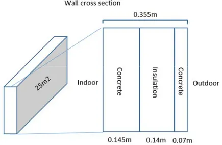
The wall component in the building model is developed according to the equations in this section. The wall measurements and composition is displayed in Figure 8, dimensions of the wall are taken for a typical residential building from blueprints by Paroc.se (2016).
Figure 8 - Modelica library development - Wall cross section
Four equations are used to calculate the temperature of the air inside the building. To determine the boundary condition of the wall equations (33) and (34) are used.
∙ ∙ ∙ ∆ ∆ ∙ ∙ ∙ ∙ ∙ 2 (33) ∙ ∙ ∙ ∆ ∆ ∙ ∙ ∙ ∙ ∙ 2 (34)
Where index w indicates the surface wall, is the density, is the specific heat, is the distance between each node, is the thermal conductivity, is the mixed heat transfer coefficient of the surface, is the emissitivity of material used in the wall and is Stefan-Boltzmann constant.
Considering the temperature profile inside the building’s wall a for-loop is used. The for-loop contains equation (35), which calculates each nodes temperature.
As all temperatures of the wall profile are known by previous equations, the indoor temperature can be calculated by equation (36).
∙ ∙ ∙ ∙ ∑
(36)
Where is the variable for the indoor temperature, is the heat transfer coefficient of air,
is the temperature of the inside boundary of the wall, is the specific heat of air, the
density of air, is the total inside volume of the building and ∑ is the summarized heat input from building mass and radiator.
4.5.2.2.
Ceiling and floor
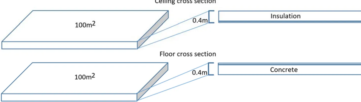
The ceiling and floor components in the building model are developed according to the measurements and equations in this section. The ceiling and floor measurements and compositions are displayed in Figure 9, where dimensions are taken from blueprints found at Paroc.se (2016). For the simulation, boundary material has been neglected and the ceilings and floors are treated as a lumped component during the calculations.
Figure 9 - Modelica library development - Floor and ceiling cross section
As mentioned the floor and ceiling are treated as a lumped components, which means that no node system is used during the simulation. Instead volume of the material used is used and uniform temperature is calculated. Looking at the floor calculations, the temperature of a uniform concrete floor is calculated according to equation Error! Reference source not
found..
, ∙ , ∙ ∙ , ∙ , ∙ , ∙ , ∙ , , (37)
Where index f, c is referring to floor or ceiling depending on what is being calculated, index s,
o refers to soil or outdoor, , is the specific heat of floor or ceiling material, , is the density of floor or ceiling material, is the mixed heat transfer coefficient, , is the surface area of the floor or ceiling, is room temperature and , is the temperature of the soil beneath the floor or outdoor temperature.
The temperature of the floor and is then used to calculate the heat transfer either to or from the floor and ceiling depending on the inside and floor temperature. It is done by equation (38).
, ∙ A, ∙ T, T (38)
Where is the mixed heat transfer coefficient, , is the area of the floor or ceiling, , is the temperature of the floor or ceiling and is the temperature of the room.
4.5.3 Radiator
To be able to simulate additional input of heat, a component of a radiator is developed to act as a heat source in the room. Both radiation and convection heat transfer is taken into consideration in the radiator component according to Reynders et al. (2012) and G. Reynders, Nuytten, & Saelens (2013).
The radiation ( ) and convection ( ) that is emitted to the room is calculated by equation
(39) and (40).
∙ ∙
(39)
1 ∙ ∙
(40)
Where is the heat emission fraction, is the heat emission coefficient, is the temperature of the radiator and is the room temperature.
Then by summarizing them both, the total transmittance from the radiator is calculated according to equation (41)
(41)
To determine the temperature of the radiator a heat balance between the water inside the radiator and radiator mass is used according to equation (42).
∙ m ∙ T , T , C ∙ ∂T ∂t (42)
Where is the specific heat of water, is the water mass flow, , is the water temperature of the radiator inlet, , is the water temperature of the radiator outlet and
4.6 Validation of model components
The validation of the components in the model is done by comparing simulated values to real-life data or literature.
4.6.1 Validation of the district heating pipelines
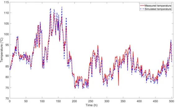
Validation of the pipelines was done by comparing measured data to simulated results. To validate the temperature distribution of the water being transported through the pipe, measured data from a 4km pipe was used. Exact properties of pipe material are unknown, but as Figure 10 displays the general characteristics of the temperature behavior shows to be valid. The data for district heating pipes are listed in APPENDIX .
Figure 10 - Modelica library development - Validation of district heating pipes
As exact properties of measured pipe data are unknown, smaller margins in the results are neglected. However, as both inlet and outlet temperature, as well as the mass flow, is known in measured data. A similar temperature curve throughout the pipe gives a good validation since the temperature lines are aligned.
4.6.2 Validation of the building
A way of validating the building’s thermal dynamics is by calculating the thermal time constant. By comparing the model’s time constant to similar buildings from literature, the thermal properties of the building is validated.
The time constant is based on the characteristics of the building. According to Antonopoulos & Koronaki (2000) it is defined as “the time needed for the indoor temperature which differs by ΔT from the outdoor temperature to change a specified amount under load”. This is seen as a thermal delay to see how long it takes for a building to react to temperature change. Different time constants for different building types are listed in Table 4.
Table 4 - Modelica library development - time constants
The time constant can according to Karlsson (2012) be used to calculate the time it takes for a building to decrease in temperature without any heating.
∙
,
(43)
Where is the temperature at time t, is the time constant, is the indoor temperature, is the outdoor temperature and , is the initial indoor temperature.
Then solving for , to be able to insert the time it takes for the model building to change in temperature. , (44)
The model is set to cool down without any added heat with an outdoor temperature of 0˚C, an initial indoor temperature of 24˚C and a target temperature of 1˚C. With these values, the modeled building has a time constant of ~310h.
Different time constant in buildings
Building type: (h) Source:
Tower block 218‐330 (Kensby, Trüschel, & Dalenbäck, 2015b) Two floor (100m2) 303 (Mejri, Peuportier, & Guavarch, 2013)
5 RESULTS
5.1 Building temperature dynamics
During investigations of the different temperatures of the building, three cases have been simulated. The cases are simulated to visualize the temperature dynamics of the building material in floor, ceilings and wall. In the cases, comparisons between different thicknesses of wall material are investigated. The thicknesses investigated are the original thickness shown in 4.5.2.1, and a case where all material thicknesses are doubled. The case differences are that case 1 simulates the building temperature when no extra heat is charged and outdoor temperature is 0˚C, case 2 simulates a case when no extra heat is charged and the outdoor temperature changes from 10˚C -25˚C after 30 hours of simulation and case 3 shows the simulation results where a charging period during night hours of 22.00-06.00 is introduced and the outdoor temperature is 0˚C.
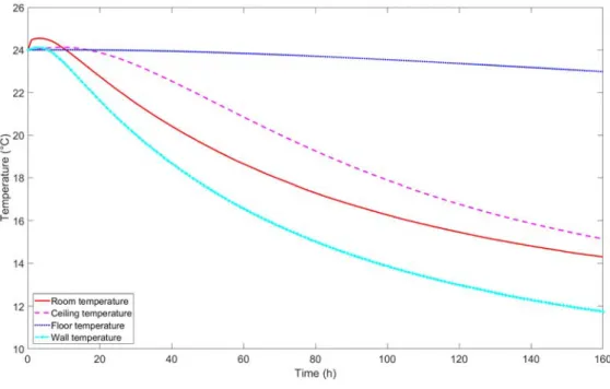
Case 1 visualizes the dynamic behavior of the building when no charging takes place and the outdoor temperature is 0˚C. Figure 11 shows the simulated results when original dimensions of wall material are used.
Figure 11 - Results - Case 1 original walls
Here it can be seen that the indoor room temperature is dependent on the wall boundary temperature, as the wall temperature is moving towards 0˚C faster compared to the room temperature.
In Figure 12, case 1 is simulated, but the thickness of wall material has been doubled. As seen in the figure, a slower decrease in temperature is reached.
Figure 12 - Results - Case 1 thicker walls
Here it is seen that the room temperature is higher than the other materials. This is because of the added temperature from the radiator. However, it shows that both wall and ceiling temperatures follow the room temperature when it exceeds their value.
During simulation of case 2, the outdoor temperature adjusting to seeing how temperatures of building materials adapt. The temperatures simulated are approximately 40 hours with an outdoor temperature at 0˚C, which at 30 hours is increased to 25˚C. In Figure 13 it can be seen that the material’s temperature adapts to the increased outdoor temperature.
Figure 13 - Results - Case 2 original walls
In Figure 13 it is seen that the indoor room temperature is constantly higher than the wall temperature, which indicates that the temperature of the room has smaller losses compared to when the outdoor temperature is increased. It can also be seen that the temperature of the ceiling is dependent on the indoor temperature with a delay. This shows that the material volume of the ceiling adapts to the change of indoor temperature. The temperature of the floor mass is marginally affected by the indoor temperature, due to a different material than the wall and ceiling.
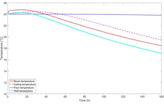
As Figure 14 visualizes the thickness of wall material has been increased, which shows that the indoor room temperature suffers from smaller losses. With thicker material, it is seen that the indoor temperature decreases by approximately 0.5˚C during 30 hours of 0˚C outdoor temperature.
Figure 14 - Results - Case 2 thicker walls
In Figure 14 it is also seen that a delay of increase in the different material temperatures is found. The outdoor temperature increases from 0˚C to 25˚C after 40 hours of simulation, but as seen in the figure, temperatures of the material volume begins to rise after 50-60 hours.
As Figure 15 shows, increased load from CHP plant is introduced during night hours. The hours where the load is increased are between 22.00-06.00 for each day.
Figure 15 - Results - Case 3 original walls
In Figure 15 it can be seen that during charging hours the room temperature increases. However, the wall temperature has a reduced decline during these hours. This is because the outdoor temperature has a significant impact on the wall temperature.
In Figure 16 the impact of thicker walls in the building material is shown. It shows that a slower decrease in indoor temperature is reached, it also indicates that the wall temperature is more affected by the indoor temperature due to thicker insulation and outer concrete layer. This gives the outdoor temperature a smaller impact on the inside wall layer.
Figure 16 - Results - Case 3 thicker walls
It is also shown that during second charging period the indoor temperature increases above the ceiling temperature, which leads to a marginally lower peak of indoor temperature because heat is in that case being transferred from the room air temperature to the ceiling material.
5.2 Radiator emission and building losses
Figure 17 shows how the outdoor temperature affects the building heat losses and the heat that is emitted from the radiator. It displays the impact on how the cold outdoor temperature increases the heat losses through the building, which is resulting in an increase in heat from the radiator.
5.3 Supply temperature delay
Figure 18 displays the pipe supply temperature time difference. The hot water is generated in the CHP plant (red line), then by distributing it into the DHN into the pipe (magenta line) and then at the end of the pipes at the consumer (blue line). It displays the time difference between the heat at the CHP plant and when the heat is delivered at the consumer 4km away. The temporary increase in temperature by the red line represents a done to increase the visibility of the dynamics. The delay for when the heat is entering the pipe and reaching the consumer is between 1h and 2h, depending on the temperature leaving the CHP plant. The time difference between supplied and delivered temperature are dependent on the mass flow of water. The mass flow used in simulations is 15 kg/s.
6 DISCUSSION
6.1 Method evaluation
The modeling and simulation method in this degree project was based on a continuation of a previous existing Modelica model. The model was developed in the program Dymola (Modelica). Model limitations in Modelica are partly based on the choice of complexity and level of detail that the modeler chooses. A lot of the coding and equations is therefore done by hand, even though there are a lot of pre-built components in the program already. Therefore the pro and also a con with the simulation tool is that there are very few limitations other than the ideas of the modeler. An alternative would have been to develop the model in a simulation tool with a 3D environment. For example, IDA ICE could be used since it handles indoor climate simulations. TRNSYS is another software that handles transient system simulations, which can be used for dynamic calculations.
The model could have been developed utilizing another type of thermal storage. For example, a thermal storage tank may yield better heat demand control and potential heat security, but the scalability of the technology would have been lower. The investment cost would also have been much higher since there would have been a substantial investment for a potential thermal storage tank. The solution with utilizing the thermal mass as storage is, therefore, environmentally- and economically friendly.
The choice of what type of thermal storage that the degree project was going to focus on, were done by researching and comparing different storage solutions. Analysis of the technologies is summarized in Table 2. Thermal storage tank is a good way of storing thermal energy in a district heating system. The containers act as a large buffer to inject hot district heating water when needed. The storage medium in the storage tank is the district heating water. The downside is the large investment cost the size of the containers is usually quite big. Another storage technology is the borehole TES. It has similar storage medium cost since it utilizes water. Its advantage is that it recovers geothermal heat, which is technically free energy. The downside to this solution is the investment cost; it cannot be applied to any larger portion of a city without it being too expensive. The latent and chemical storage have similar advantages. One being the high storage capacity per volume, which makes it a good option when it comes to space limitations. Another advantage is their high performance and low losses. The consequence of this being the high cost of PCM and chemicals. On a larger scale, the investment cost makes it too expensive. The technology we chose to develop further is the thermal mass storage. The main reason being the scalability of the technology and the non-existent investment cost. This is because it utilizes the already existing building mass as a storage medium and it can be applied and be up-scaled on large portions of a city area.
6.2 Validation
The validation of the district heating pipes is made by trying to replicate a part of the already existing DHN of Mälarenergi’s. By taking a section of their piping system and comparing the temperatures in a 4km pipe shown in section 4.6.1. This method gives us confirmation of the heat propagation and heat delivery time difference. The piping data and properties that are used is showing proper temperature and time resemblance. If the valleys and peaks had not been as aligning, the simulation would have represented inaccurate thermal delay. However, as visualized in Figure 10, it simulates good dynamics when it comes to the heat delivery time difference from producer to consumer. It can also be seen that the calculated temperature compared to the simulated temperature in the district heating pipes still shows a little inequality at some points, this might be due to wrong pipe properties in the model or a measurement deviation.
Validating the building dynamics is done by comparing the time constant. The time constant displays the building’s properties to react to temperature change. The calculated time constant is compared to other time constant in the literature, displayed in Table 4. The model’s time constant of 310h is similar to the time constant of a two-floor building with 100m2 of floor area, which has 303h. A tower block time constants ranging from 218-330h is
also within range of the building model’s time constant. This verifies that the model heat dynamics and thermal inertia is working correctly.
6.3 Model limitations
As the model is limited by not taking losses by ventilation or leakages into account the simulated heat losses may not be as accurate as a real-life building. However, as the model's purpose is to give a visualization of the ability to store heat in thermal mass, these losses can be neglected and still show the impact of the amount of building mass.
One limitation that the model development faced were the limitations in the program Dymola. As the student-version was used during simulations, error messages occurred when using too many equations in a model. Therefore, were we forced to decrease the number of nodes in heat equations in walls and pipes. This may not have a significant impact on the overall results, but by increasing the number of nodes within the simulations, it will show a higher accuracy of heat transfer.