I
School of Innovation, Design and Engineering
Reducing Inventory and
Optimizing the Lead time in
a Custom order, High model
mix Environment
Master thesis work
30 credits, Advanced level
Product and process developmentProduction and Logistics
Shilpashree Dayananda Salian
Report code: PPU503
Commissioned by: Atlas Copco Rock Drills AB Tutor (company): Nicole Schoch
Tutor (university): Antti Salonen Examiner: Antii Salonen
II
ABSTRACT
In this contemporary world, demand forecasting has become an effective tool for the success of any product organization. This is especially important when their components have long lead times and when the companies don’t build on order. The goal of this thesis is to reduce inventory by improving the forecast accuracy while maintaining customer lead time in a custom order, high mix model environment.
In this master thesis investigation, the research questions that were formulated are answered individually. To be able to answer the research questions, a thorough literature review was done to understand the various findings within this research area. In this thesis, only the high cost commodities were considered such as engines and frames as it costs an arm and a leg to have these high cost commodities in stock. Additionally, under estimating the forecast values of these components can be detrimental to business as the lead time of these high cost commodities are too long.
Firstly, the forecasting accuracy of previous years’ data is calculated and measured through forecast error measuring parameters such as cumulative forecast error, mean squared error, standard deviation of error, mean absolute deviation and mean absolute percentage error. In the empirical findings part of the thesis, the problems faced with the existing forecast method is briefed which highlights the root causes for overall forecast inaccuracy. Aforementioned forecasting problems inevitably increase the inventory level which is a serious threat to an organization due to working capital tie up.
Secondly, a hypothesis model was developed as an alternate forecasting model by considering the demand patterns from the past three years (historical) data. By analysing the demand pattern it was clear that the nature of the demand has been lumpy. A hypothesis model known as Croston’s model was developed and by applying the historical demand values, the forecast values were calculated. A key performance indicator known as mean absolute scaled error was calculated for both the existing and Croston’s forecast method for the purpose of comparison. The results proved that the Croston’s method gives better forecast accuracy when compared with the existing forecast method.
And finally, to improve the forecasting process as a whole, a benchmarking study has been successfully carried out. The benchmarking study is done with three internal companies within the Atlas Copco Group. The companies have been chosen by looking at the similarity in their product portfolio and business challenges faced
(Keywords: Forecasting, inventory management, forecasting methods, forecast accuracy lumpy demand)
III
ACKNOWLEDGEMENTS
I take this opportunity to thank all the wonderful people who have been part of my thesis sojourn.
Firstly, the friendly associates at Atlas Copco Rock Drills AB, my supervisor Nicole Schoch and mentor Kent Blom for providing the opportunity to carry out this study as well as tirelessly supporting with the inputs and constructive suggestions. Really, thank you!
I will miss fikas!
Secondly, my lecturers at Mälardalens University, especially to my guide Professor Antti Salonen for spending his valuable time answering my queries and guiding me in the right path. Thank you for anticipating the research and industrial requirements and empowering students accordingly. I should mention that the synergy between the university and the industries during my course work is really admirable.
Last but not least thanks to my dearest family for supporting in my endeavours.
Shilpashree Eskilstuna, 2016
IV
Contents
1. INTRODUCTION ... 1
1.1. BACKGROUND ... 1
1.2. PROBLEM FORMULATION ... 2
1.3. AIM AND RESEARCH QUESTIONS ... 3
1.4. PROJECT LIMITATION ... 3 1.5. PROJECT OUTLINE... 3 2. RESEARCH METHOD ... 5 2.1. METHODOLOGICAL CHOICES ... 5 2.2. CASE STUDY ... 5 2.3. CASE COMPANY ... 6 2.4. DATA COLLECTION ... 6
2.4.1.PRIMARY AND SECONDARY DATA ... 7
2.4.2.LITERATURE STUDY ... 7
2.4.3.BENCHMARKING ... 8
2.4.3.1. INTERNAL BENCHMARKING V/S EXTERNAL BENCHMARKING ... 9
2.4.4.INTERVIEWS ... 9 2.5. HYPOTHESIS TEST ... 10 2.6. QUALITY OF RESERACH ... 10 3. THEORETICAL FRAMEWORK... 12 3.1. FORECASTING ... 12 3.2. FORECASTING METHOD ... 14 3.2.1.QUALITATIVE METHOD ... 14 3.2.1.1. MARKET STUDY ... 14 3.2.1.2. SALESFORCE ESTIMATES ... 14 3.2.1.3.EXECUTIVE OPINION ... 15 3.2.1.3.THE DELPHI METHOD ... 15 3.2.2.QUANTITATIVE METHOD ... 15
3.2.2.1. STATISTICAL DEMAND ANALYSIS ... 15
3.2.2.2. TIME SERIES METHOD ... 15
3.2.2.2.1.SIMPLE MOVING AVERAGE ... 16
3.2.2.2.2.WEIGHTED MOVING AVERAGE METHOD ... 16
3.2.2.2.3.EXPONENTIAL SMOOTHENING METHOD ... 17
3.2.2.2.3.1.TREND BASED EXPONENTIAL SMOOTHENING METHOD ... 17
3.3. FORECAST ERRORS ... 17
3.4. FORECASTING METHOD FOR LUMPY DEMAND ... 19
3.5. CROSTON'S METHOD OF FORECASTING ... 19
3.6. IMPROVING FORECAST ACCURACY ... 20
3.7. STRATEGIC RESOURCE PLANNING (SRP)... 21
3.7.1.IMPORTANCE OF SALES FORECASTING FOR SRP ... 22
3.8. INVENTORY MANAGEMENT ... 22
3.8.1.ABCCLASSIFICATION ... 24
4. EMPIRICAL EVIDENCE... 25
4.1. THE COMPANY ATLAS COPCO ... 25
4.2. SRP FORECASTING AT ATLAS COPCO ... 27
4.3. EMPERICAL RESULT ... 28
5. HYPOTHESIS TESTING ... 31
5.1. INITIALIZATION OF A HYPOTHESIS ... 31
5.2. PURPOSE OF BUILDING A HYPOTHESIS ... 32
5.3. HOW THE HYPOTHESIS TOOL WORKS ... 32
5.4. RESULTS FROM HYPOTHESIS TEST ... 34
V
7. PROCESS BENCHMARKING ... 42
7.1. ATLAS COPCO COMPANY A... 42
7.2. ATLAS COPCO COMPANY B ... 42
7.3. ATLAS COPCO COMPANY C ... 43
8. CONCLUSIONS... 45
9. FUTURE WORK ... 46
10. REFERENCE ... 47
11. APPENDICES ... 52
List of Figures:
Figure 1- Fish bone diagram for forecast accuracy 2Figure 2- Benchmarking stages 8
Figure 3- Level demand pattern 13
Figure 4- Trend demand pattern 13
Figure 5- Seasonal demand pattern 13
Figure 6- Cyclic demand pattern 13
Figure 7- Random demand pattern 13
Figure 8- Simple moving average 16
Figure 9- Flow of information between three levels of SRP 22
Figure 10- ABC Classification 24
Figure 11- Classification of different business units under MR 25
Figure 12- SRP forecast at Atlas Copco 27
Figure 13- Engine 29
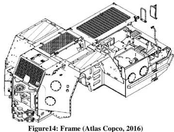
Figure 14- Frame 30
List of Tables:
Table 1- List of respondents for Benchmarking 9Table 2- Product range of URE 26
Table 3- Forecast error measure for engines 29
Table 4-Forecast error measure for frames 30
Table 5- Croston´s model 32
Table 6- Calculation table 33
VI ABBREVIATIONS
AC Atlas Copco
AFE Average forecast error
CC Customer centre
CFE Cumulative forecast error
ERP Enterprise resource planning
KPI Key performance indicator
MAD Mean absolute deviation
MAPE Mean absolute percentage error
MASE Mean absolute scaled error
Mdh Mälardalen University
MRE Mining and rock excavation division
MRP Material requirement planning
MRS Mining and rock excavation services
MSE Mean squared error
OR Operation research
RCS Rig control system
SED Surface exploration drilling
SDE Standard deviation of error
SRP Strategic resource planning
SS Safety stock
1 1. INTRODUCTION
This chapter includes background, problem formulation, aim, research questions, project limitation and an outline of the thesis work is presented.
1.1 Background
Supply chain management is a theory that has evolved since the past few decades to enhance trust and partnership among the supply chain partners for better service and improved efficiency. The term “supply chain management” has become a buzzword in operations management strategy since early the 1980’s. According to Levy & Weitz (2009), in the supply chain retailers play a prominent role as they build a close link between the suppliers and the customers to ensure that goods are received on time and in the right quantity.
“Supply Chain Management consists of developing a strategy to organize, control and motivate the resources involved in the flow of services and materials within the supply chain” (Krajewski et al., 2006, p.372).
Davis (1993) mentions that in the supply chain system, there are various time derivative functions which often fluctuate and this affects the supply chain environment. One of the time derivative functions is the forecast. Due to the globalization and increased competitiveness, it is hard to predict the optimal forecast. It is a challenge for the manufacturing industry to deal with the imbalance between the forecast and the demand. Inventory management is an integral part of the logistic system within the supply chain. Well-functioning inventory management plays an important role in measuring the organization’s ability to function with greater profit margin. Van Hoek et al (1998) mentioned that in the recent days, demand is one such variable which is tedious to forecast because of varying customer requirements. Due to the changing market condition and increased customer needs, the products need to be available with improved quality and sufficient quantity. The increased forecast inaccuracy has a greater impact on the inventory management. The inventory planning is dependent on the forecast made i.e. the estimation made to sell that many products. When the demand decreases, the stock level increases which results in decreased profit levels, losses can incur in the worst case.
The top level management in many organizations constantly faces problems in the strategic planning and decision making (Thomopoulos, 2015). The root cause for these problems is the uncertainty in the demand creating a challenge for the industries to improve their forecasting accuracy. Now with the improved technology, industries are allocating resources to measure their forecast accuracy and thereby trying to improve on that front. It can be noticed that there are various demand patterns which include smooth, intermittent, sporadic, lumpy etc. (Syntetos, et. al., 2005). Among these, the lumpy demand is the trickiest of all, and it has made the inventory planner´s life more difficult. Moreover it’s even more challenging for the organization to predict the forecast for those items which have lumpy demand for longer periods.
Hyndman (2009) defines forecasting as a process of “predicting the future event by relying on the availability of the past data”. According to Arnold et al., (2007), the forecasting is done for various purposes to meet the future demand. The important purpose is to be cost efficient and to have a sound production and resource plan. By estimating the forecast
2
beforehand, it is possible to have the stock availability so that the products/services can be delivered to the customers at the earliest. The advantage of forecasting is that, it can reduce the production cost and have high service level and customer satisfaction (ibid).
According to Wallström & Segerstedt (2010), it is a challenge to build a flexible forecasting method to deal with the changes in the market condition. The effect of increased forecast error from the strategic plans is a critical issue, this makes a negative impact on an organization’s business economy and it has been a topic of interest for researchers (Holt et al., 1955). In the recent days the research studies based on improving forecast accuracy have gained popularity as it improves the economic status of organizations (Ritzman & King, 1993).
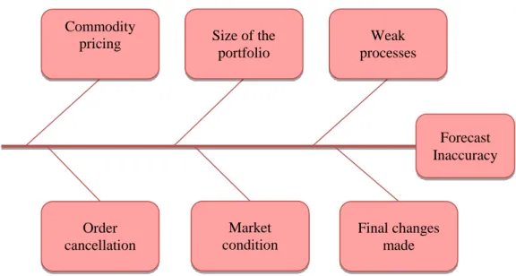
To get a clear understanding of the background of this problem and to highlight the root causes for the existing problem, a fish bone diagram is used. Below figure 1 shows the various root causes for the forecast inaccuracy.
Root cause Analysis
1.2 Problem formulation
The root cause analysis shown above serves as a framework to formulate the problem in a better way. The biggest hurdle for any organization/industry would be meeting their customer demand in terms of service level and lead time by maintaining low inventory level. Inventory management plays a major role as it balances inventory and material availability. The root cause for the chain of problems is by following an inaccurate forecast. In this thesis, one of the main objectives is to shorten the product lead time for high mix low volume customized machinery.
Most of the product manufacturing companies especially within the mining sector employ the strategy of purchasing items on marketing forecast but with many variation and changes
Forecast Inaccuracy Commodity
pricing Size of the portfolio Weak processes Market condition Order cancellation Final changes made
3
this results in high inventory levels. The task is to analyze how forecasting can be effected looking only at long lead time/high cost items and what forecasting model can be used, assuming no accurate marketing forecast is available. The overall goal is to reduce or maintain equipment lead time while reducing inventory.
1.3 Aim and Research questions
The aim of this thesis is to build a reliable forecasting model for companies with highly customized products with an intermittent/lumpy demand. In order to serve the aim of this thesis, the following research questions have to be answered.
Research question 1:What is the existing forecasting system at the case company and what are the problems faced with the existing forecasting system?
Research question 2: How accurate is the forecasting done by the case company in the past years?
Research question 3: Which existing forecasting models are there for handling lumpy demands?
Research question 4:What is the best alternate forecasting method that can be implemented to deal with the inventory issues?
1.4 Project limitations
This thesis work was performed in a span of 20 weeks from 2016-01-14 to 2016-05-31. Due to the limited time period, data collection for this project was limited and only few components were selected for forecast analysis. Further as a part of this thesis work the benchmarking was done and due to limited time the benchmarking done was only with 3 companies within the Atlas Copco Group. The external benchmarking was considered in the planning stage of this project, however all the companies who we contacted, with similar product portfolio were reluctant to share any information and therefore it is not a part of this thesis.
High level mathematical analysis is not a part of this thesis as the student’s mathematical knowledge is limited; having said that, the mathematical approach is used to derive many answers in this study but not to the advanced concept level.
1.5 Project Outline
This thesis report is split into six segments. At the outset, the methodology implemented to perform the study is explained. The next part sheds some light on the detailed literature review and the appropriate theory to understand the study. The data gathered in this study is used in the third part i.e. the empirical findings and later the result is presented. In order to get deep into the research question, hypothesis testing has been done and it is presented in the next section. To ensure the theory studied in this study is answerable to the research
Main problem: How to deal with inventory build-up problems by improving forecast accuracy when there is
4
questions, a clear analysis is done and it follows in the next section. To take this study into the next level a benchmarking study is done, it is presented in the next section. Last but not the least, the final part of the report is of course the conclusion, followed by suggestions on future works.
5 2. RESEARCH METHOD
In this chapter, the research methodology followed in this thesis work will be elucidated. It includes the methodological choice, the case study and the research strategy used for this thesis work. And finally the quality of the research in terms of validity and reliability is justified.
2.1 Methodological choice
“Research Methodology is a systematic way to solve research problem” (Kothari, C. R., 2004, p.8).
The goal of this master thesis in general is to build an alternate forecasting model for the companies that have highly customized products with intermittent/lumpy demand. In order to build a new forecasting model it’s essential to study the existing forecasting system. To study in depth about the existing system, in this case Strategic Resource Planning (SRP) driven forecasting system, all the required qualitative data had to obtained and studied. The historical quantitative data was also collected and analyzed for the purpose of empirical calculation. The quantitative data is also an integral part of this case study as the new suggested model depends on the previous historical data.
By reviewing the historical SRP forecasting method the forecast errors have been calculated, and later on Croston’s method has been used as a hypothesis tool. It is built in order to check if the forecast values yield better accuracy. Based on the literature studied, the hypothesis analysis was done to check the forecast accuracy. As a further step, the benchmarking process was also executed within the sister companies to review the potential performance improvement. Here in this thesis work, only process benchmarking is considered.
2.2 Case study
Ejvegård (2003) mentioned that reliability is often regarded as a precision measurement tool. He also stresses on the fact that the case study enables the researchers to focus on a particular problem and identify its connected roots and causes. In this thesis work, the case study is performed through benchmarking to study the forecasting process. The benchmarking process is explained in detail under the section 2.4.2. As a part of the research approach, the case study has been done in three internal benchmarking to deeply study the forecasting process and analyze the gathered information. Case study is used in various fields such as medicine, finance, manufacturing and many more. The purpose of performing a case study is to get a better understanding of a complex situation. According to Yin (2003), case study permits the researchers to maintain a reliable and holistic view of the day to day life affair. In short, it is a process of study in length and depth instead of breadth or width (Kothari, 2004).
The case study is mostly preferred for the qualitative research and it mainly focuses on the detailed investigation with a contextual setting approach. Case study is beneficial to deal with the qualitative research as it can be used to study in depth about the processes in the industries (Bryman & Bell., 2011). The qualitative case study enables the researchers to analyze the complex case by fragmenting it into segments within their area of specialization (Baxter & Jack, 2008). By performing the qualitative case study, the research topic gains
6
multiple visions to explore, which make it possible to disclose the multiple aspects to be studied and analyzed (Yin, 2003). The reason behind choosing the case study for this thesis work was to study the forecasting process of three internal companies within the Atlas Copco Group.
2.3 Case Company
The case company in this thesis work is Atlas Copco Rock Drills AB. Atlas Copco Rock Drills AB is a part of the Swedish industrial group Atlas Copco. Atlas Copco Group is a world leading provider of sustainable productivity. The parent company was founded in the year 1873. Atlas Copco Group companies have their headquarters in Stockholm, Sweden and the group is active in four main business areas, they are:
1. Compressor Technique
2. Mining and Rock Excavation Technique 3. Industrial Technique
4. Construction Technique
The Atlas Copco Group has close to 100 production sites in nearly 20 countries. It has ca 45 000 employees in 90 different countries and has its customers in nearly 180 countries. Sustainability and innovation are the core mantra of Atlas Copco. (Atlas Copco, History, 2016)
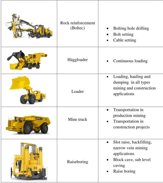
Atlas Copco Rock Drills AB comes under the umbrella of Mining and Rock Excavation Technique or Mining and rock excavation business area (MR) division. The company is based out of Örebro in the central part of the Sweden where it has its production facilities. At Örebro facility, they research, develop, manufacture and market rock drills, rock drilling rigs, trucks and loaders. Their products are used in both under and above the ground applications for mining, tunneling and construction purposes. They emphasize on customer service so there is a separate service division to be “first in mind- first in choice” (Atlas Copco Rock Drills AB, 2016).
Atlas Copco Rock Drills AB at Örebro can be further broken down into 4 divisions namely Rocktec, Underground Rock Excavation (URE), Surface and Exploration Drilling (SED) and Mining and Rock excavation Services (MRS). My thesis is carried out at URE division.
2.4 Data Collection
For an effective case study the data collected should be highly reliable else it can turn to be futile. Yin (2003) mentions that to perform a successful case study the researcher must possess excellent skills in the specialized area of research. The researcher should have the ability to extract the required data and find relevant sources to gather information. Gathering the data is a very crucial process in any research work. The data can be qualitative or quantitative in nature. The qualitative data is purely theoretical and it is mainly obtained by interviews, observation, books etc. The quantitative data is usually numerical and it is obtained from database sources such as company’s historical log book, e-files, transaction files etc. (Yin 2003, Trochim, 2006).
But to actually get started with the research process, it is important to study the literature in detail and identify the key areas in literature to perform the research. In this thesis work the case study is split into two segments. Firstly, the historical data have been collected from the
7
company’s Enterprise resource planning (ERP) system. Data from the year 2013 to 2015 was chosen for this analysis. Since the case company had loads of data, it is too tedious to slice the data for all the components. Hence only a few crucial high cost components were shortlisted for this study such as engines and frames. Thereby narrowing it down to few suppliers, the historical data was obtained, both the actual demand and the predicted forecast. Secondly, the case study in terms of the benchmarking process has also been performed. In this approach the information is gathered through interviews, emails, telephone meeting etc.
2.4.1 Primary and Secondary data
The data can be obtained both from primary and secondary sources. The data gathered by direct means or in person by observation or interviews is referred to as primary data. Data obtained from previous works i.e. mainly thesis reports, journals etc. is referred as secondary data (Kothari, 2004; Saunders et al., 2012). The availability of secondary data has been made easy in the past few years due to technological improvement or growth. Due to easy accessibility to research publication databases, it aids the researchers to obtain the secondary data sources (Bell, 1999).
It is essential to study the secondary data to get started and understand the theory behind the research topic even though the research work is mainly dependent on the primary data collected. But the secondary data can be used to analyze the result obtained from the research work which was obtained by using the primary data (Kothari, 2004). Usually in any research work both the primary and secondary data will be used by the researchers (Saunders et al., 2012). In this thesis work, the primary data is obtained through interviews, telephone and Webex meetings. It is explained in the section 2.4.4. The secondary data is obtained from the databases of Mälardalens University (Mdh) and the documents that were accessed from case company’s homepage.
2.4.2 Literature Study
Literature study is the review of existing knowledge on a particular topic from various sources such as journals, articles, books, university database, library etc. (Hart 1998). It includes information such as the root source from where the specific literature has been extracted and its background information. In the literature review, there always exists a flow in the information which is useful to get a clear view of the topic and to proceed further in the investigation process. According to Kothari (2004), the literature study serves a backbone to perform the empirical calculations and achieve the results. By performing literature study, it makes one to easily understand the research problem and also to improve the overall methodology in the research work. Saunders et al., (2012) also mentions that dissertation reports and scientific journals aid to get a clear understanding of the theory behind the relevant area of research.
The summon database of Mdh, google scholar, web of science, science direct, ABI/INFORM global, Scopus were some of the databases that were used to find the appropriate literature by using the key phrases such as forecasting, forecasting method, forecast accuracy, lumpy demand, inventory management etc.
This paper mainly focuses on building a forecasting model to improve the forecast accuracy when there is an intermittent demand. Hence many related articles on forecasting accuracy
8
have been studied deeply and explored. Also theory on benchmarking has been studied for further process investigation.
2.4.3 Benchmarking
“Benchmarking is the process of continuously evaluating and comparing one’s business process against comparable process in leading organizations to obtain information that will help the organization identify and implement improvements”(Andersen & Pettersen,1995, p. 4).
Camp (1989) emphasizes that benchmarking is one of the powerful tools to review the best practices adopted by the industries to improve the overall performance. He stressed on the fact that the organizations observe the key business processes and tries to match their performance with the benchmarking organization. For example, most of the automotive industries have benchmarked with Toyota industries and have adopted their lean methodologies. According to Longbottom (2000), the benchmarking process is mostly done to improve the quality of the process. The four main stages in the benchmarking process as per Deming’s (1986) quality cycle are: Planning, Analyzing, Implementation and Review (ibid).
The figure below shows the different stages in benchmarking process.
Figure 2: Benchmarking stages (Czuchry, et al., 1995, p.39) Benchmarking process can also be categorized into 3 types, they are:
External benchmarking
Internal benchmarking
Generic benchmarking
External benchmarking deals with evaluating the process with other organizations but within the same industry. Internal benchmarking is evaluating the process with a different department, division or business unit but within the same organization. Generic benchmarking deals with evaluating and analyzing the performance from a different organization and industry. But the core concept of all three types of benchmarking processes deals with understanding the process, observation, evaluation and analysis of the performance measures (Longbottom, 2000).
Think Act Evaluate Plan Look ahead
9
2.4.3.1 Internal benchmarking v/s External benchmarking:
“Spend your time looking in the mirror, not out the window”(Puckett III & Siegel, 1997, p.15).
Internal benchmarking can be used in large organizations where they have multiple business areas and different divisions which can be analyzed and compared with one another (Andersen & Pettersen, 1995). Internal benchmarking is used to compare the organizations working process internally. The company should be familiar with its own products, working principles, core values, etc. in order to compare with other organizations. It is the best practice to improve their process within the organization (ibid). The advantage of internal benchmarking is ease of access to data (Spendolini, 1992).
List of Respondents for Benchmarking:
Company Position of Respondents
Atlas Copco Rock Drills AB
Supply chain Manager, Regional business Support,
Production Planning & Purchasing manager Atlas Copco
Company A
Logistic and Planning Manager Atlas Copco Company B Process Manager, Forecast to invoice Atlas Copco Company C Order-ToDelivery Manager
Table 1: List of respondents for Benchmarking 2.4.4. Interviews
Gathering information from interviews is one of the key sources to perform any research work (Yin, 2003).To get started with the benchmarking process it is important to prepare a set of interview questionnaire in order to gather the required information. Even though there are multiple ways to collect the information while performing a benchmarking process, it is stated that interview is one of the best practices (Andersen & Pettersen, 1995). The interview method requires minimum two persons i.e. the interviewer and the interviewee. Kothari (2004) mentions that there are two types of interviews conducted in a research process they are personal interview and telephone interview. He also mentions that the motive of conducting the interviews is that it should sway the research design and purpose.
o Personal interview: A personal interview is a method implemented in the qualitative research to gather information from the concerned authority. It is a conversation between two or more individuals in person. In this method the interviewer prepares a
10
set of questions in advance and asks the interviewee and gathers all the needed information (Kothari, 2004). This method is mostly preferred for intensive research analysis. In this method, the process of gathering information is done in a more structured manner.
o Telephone interview: A telephone interview method is also used to gather information for the research purpose. It is not regarded as the most common aid to perform the interview, but it is most commonly used in industry surveys when the locations are too far from each other (Kothari, 2004).
In this thesis, the interview questions were built by having a perception that it is a qualitative research. The designed interview questions were mostly open-ended which made the interviewee expressive in their answers with free flow of thoughts.
The interview questionnaires were built by intensely studying and understanding the foregoing research areas within forecasting. Also by studying relevant articles in this area to see what previous researchers have achieved and taking it a step further by involving new ideas, concepts and approaches to yield better results. It is constructed to get a clear vision about the research problem and to make it more interesting and captivating throughout the interview session. The questionnaires are included in the appendix section A.
2.5 Hypothesis test
A hypothesis test is regarded as the primary tool in research. Its purpose is to examine and experiment the available data by applying some theoretical knowledge (Kothari, 2004). According to Meriam (1988) a hypothesis test is a kind of case study that is performed to analyze the results obtained from the literature and empirical findings. There are various purposes to use the hypothesis testing, but the main purpose is to verify the findings in the research study.
In this thesis, for the first step the literature study was performed and as empiricalevidence, forecast errors were measured by following the time series forecast calculation. As a next step, Croston’s method was introduced as hypothesis tool to check for improved forecast accuracy. The mean scaled error was measured and compared with the existing forecast and forecast obtained from Croston’s method. The hypothesis testing is done to prove the model, which was built by studying the relevant literature and by analyzing it. To perform the hypothesis test, the historical data was extracted from the company’s ERP system.
2.6 Quality of Research: Validity & Reliability
The quality of the research is measured by its reliability and validity. While performing a case study, validity and reliability relies on the researcher’s potential to make a project plan and execute it, problem solving approach and development of the conclusion. According to Merriam (1998), a qualitative research should be very precise so that the reader should be able to judge the drawn conclusions are logical or probable.
Data obtained in the research study must be tested logically in order to check if it is reliable and valid. The reliability is estimated by obtaining similar results when the experimental test repeats. Bell (1999) mentioned that test-retest method is the most common tool used to check the reliability of the research work. Validity is a tool which ensures that right thing is
11
measured that was planned in the project. It is also clear that if the data is not reliable then it cannot be valid. But the author also mentions that valid data is not always reliable (ibid). The researchers build their tool for their research study and every developed tool has its own implication and they are unique. Hence the results obtained from the research study vary accordingly. Reliability in this thesis study is connected with a consideration by performing a qualitative research. Validity in this thesis is achieved by analyzing the results from the hypothesis and also by comparing it with the existing method.
12 3. THEORETIC FRAMEWORK
In this chapter the relevant literature study is covered which will be later used in the empirical part of the thesis work.
3.1 Forecasting:
Forecasting is widely used by all industries to plan their resources. By estimating the future they are better able to fulfill the customer demands (Jonsson & Mattsson, 2013). The forecasting can be seen in areas such as finance, marketing, production and the whole supply chain management. The forecast serves as an input to the planning model (Armstrong, 1985).
In this theoretical background only a few topics of forecasting will be touched, keeping the focus on improving the forecasting accuracy and method to improve the forecast accuracy. The theoretical framework includes the forecasting theory, different forecasting methods, forecast errors, how to improve forecast accuracy and performance and inventory management.
Some of the industries build their products based on the customer order received in general construction and mining industries follow certain forecasting techniques to predict the future customer demands and build their products as the customers do not wish to wait long to receive their orders (Arnold , et al., 2007). Forecasting is very essential for the decision makers when there is any uncertainty coming in the future (Armstrong, 2001). It is usually misinterpreted as planning by many, wherein planning is mainly concerned with “what the world should look like”, whereas the forecasting is mainly concerned with “what the world will look like” (ibid).
The forecasting methods can be used for the planning process to foresee the possible changes in outcomes allowing the creation of plan B/alternative plan. When right information is gathered by the planners in more structured or precise way they can have better preparation for future demands. Hence forecasting can be seen as very powerful tool in the decision making process to deal with reduction of the uncertainties that can occur (Jones & Twiss, 1978). But while choosing the forecast method one must adapt the flexibility to change their method while any lumpiness occurs in the demand. Hence it is ideal to consider the lumpiness factor while choosing any forecasting method (Ghobbar & Friend, 2003).
According to (Olhager, 2000), forecasting is done considering the previous historical data and the demand pattern may vary over the time. Hence before choosing any forecasting method it is important to consider the demand pattern. Krajewski et al (2006), mentions that a continuous occurrence of demand for any product can be observed by considering the historical data and this method of forecasting is known as time series forecasting. Thus by analyzing the repeatability in the demand under the time series, there are five different demand patterns (ibid). They are:
i) Level iv) Seasonal ii) Trend v) Random iii) Cyclical
13
The above mentioned demand patterns are illustrated in the figure below:
D D t t D D t t D t
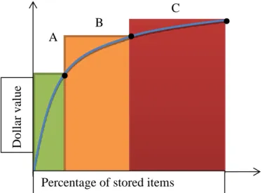
Among these, the random demand pattern shown in figure 7 is the hardest off all to forecast (Mattsson & Jonsson, 2013). It has been an interest area of research to investigate the reasons for randomness and how to overcome and measure to deal with it. Few authors have linked these demand patterns with the inventory management strategies as it deals with stocking the products when such demand patterns occurs. It has led to ABC classification of the parts in the inventory; it will be covered in the section 3.8.1 of this report.
Figure 7 Random demand pattern (ibid)
Figure 3 Level demand pattern (Krajewski et al., 2006 pp.524)
Figure 4 Trend Demand pattern (ibid)
Figure 5 Cyclic demand pattern (ibid)
Figure 6 Seasonal demand pattern (ibid)
14 3.2 Forecasting Methods:
In general forecasting approach can be categorized into qualitative and quantitative methods. The forecasting methods used in the industry today falls under the above mentioned categories. There is no such best or optimal forecast method, each method has its pros and cons. Selecting the right method depends on factors such as previous forecast history, relationship with the suppliers, product forecast etc. According to Green (2001), while focusing on product forecasts, it is advisable to adopt a combination of few forecast methods.
3.2.1 Qualitative method
The qualitative method stresses on forecasting the future rather than illustration about the past (Makridakis & Wheelwright 1989). This method is applicable when there is no sufficient quantitative data available and instead there will be ample amount of qualitative information available (Masegosa, et al., 2013). This method is known as judgmental forecast, which mostly depends upon past experience, intuition/perception and knowledge without building any explicit forecast models. It is the most adopted forecasting method in most of the product companies these days (Dyussekeneva, 2011).
If these subjective methods were not implemented then the quantitative method would give erratic forecasts (Krajewski et al., 2006). There are four main successful subjective forecast methods. They are: The Market study, salesforce estimates, executive opinion and the Delphi method (ibid).
3.2.1.1 Market Study
It is the most logical approach to gather information about the external customer needs in service or products by building and examining the hypothesis via data collection surveys (Krajewski et al., 2006). It comprises of constructing a list of interview questions, managing to grab all the possible information, choosing the right illustrative model, and mainly analyzing the gathered data either by subjective or statistical method in order to clarify the responses. Even though the market study gives the maximum useful information, it will still contain some barriers to get through (ibid).
3.2.1.2 Salesforce estimates
It is pretty clear that the foremost information about the future demand mainly comes from people who interact closely with the external customers (Krajewski et al., 2006). This forecast data is gathered from the customer centers, and they are reviewed by the sales company executives. It is regarded as a descended approach of the executive opinion method, wherein the information gathered by the sales executives or sales managers are taken into consideration for predicting the future demand (Kahn, 2003). By using these methods, there are many advantages as the salesforce is a group who are mostly highly knowledgeable about the future demand of the product/service that the customers will buy. Also, the forecast gathered by individual salesforce can be merged to find out the local, state or national sales (Krajewski et al., 2006). There are also certain drawbacks such as, for the salesforce it may be hard to interpret the difference between customer “wants” (wish list) and customer “needs” (buying list). (ibid)
15
3.2.1.3 Executive Opinion
It is a forecasting method where the judgements, views, opinions, work experience, scientific and practical knowledge of sales or production managers are merged together to attain a single precise forecast. It is a general practice when a new product or service is introduced to the market (Krajewski et al., 2006). At this instance, for the salesforce group it may be hard to make accurate forecast as it will not have any historical demand information. It is suggested that Executive Opinion is best suited for technological forecasting (ibid).
3.2.1.4 The Delphi method
It is one of the methods to obtain agreement from experts while not revealing their identity (Krajewski et al., 2006). This method is applicable when there is no availability of historical data to build any statistical models and if the managers have absolutely no background knowledge or experience to rely on the available forecast. In such cases, the concerned manager sends questions individually to everybody in the expertise group, where no personal identity is revealed of the organization or the person. The coordinator gathers the responses from every individual of the expertise group. The summary is made and further sent with more detailed queries for a second round of discussion. The process continues for few more rounds till final conclusions are made (ibid). This method is very similar to the executive opinion method as it considers the experts advice (Green, 2001).
This method is most efficient to improve long series forecast for product/service and also for forecast prediction of newly introduced products. This method is also best suited for technological forecasting (Krajewski et al., 2006).
3.2.2 Quantitative method
This method can also be regarded as an objective forecasting method. In this method, forecast is obtained mainly by data analysis (Ramström & Söderlund, 2001). The forecast from quantitative method can be implemented only when there is sufficient availability of the historical data (Krajewski et al., 2006). This historical data is known as a history file, which is stored in a certain commercial database. But when a new product is launched, then these history files may not be useful. In such instances, a subjective or judgmental forecast method may be beneficial to adjust the forecast that was gathered by quantitative methods. It is sub categorized into: statistical demand analysis model and time series method analysis.
3.2.2.1 Statistical demand analysis
This method takes into consideration the preceding and succeeding sales pertaining to the demand factors instead of considering time dependent factors. This method uses statistical approach to deal with the causing factors of sales fluctuation and other relative factors such as commodity price, revenue, advertising promotions etc. (Kotler, et al., 1999). Casual method such as linear regression method is most commonly used for statistical demand analysis. In this method it is possible to identify the influencing factors of forecasting and other relative external/internal factors (Krajewski, et al., 2006). In this method the relation between dependent and independent variable is expressed as a linear equation. It is represented as, 𝑌 = 𝑎 + 𝑏𝑋
Where, Y is dependent variable, X is independent variable, a is the y-intercept, b is slope of line (Krajewski et al., 2006 p. 529).
16
3.2.2.2 Time series method analysis
It is purely a statistical forecasting method which focuses on previous years historical data, irrespective of its correlation or bonding linked with the economic theory (Carnot et al., 2011).
This method uses the historical data concerned with only the dependent variables for the forecasting analysis (Krajewski, et al., 2006). By taking into consideration that there will be a possibility of a repeated pattern of the dependent variables the forecast values are estimated. The most common forecasting method that is adapted under time series is the naive forecast method. In this method the forecast approximated for the coming year is equivalent to the demand of the current year. For example while considering forecasting on a monthly basis, if the demand for January is 5 products then the forecasted demand for February is considered as 5 products. It is highly recommended for the demand which has seasonal trends. It is applicable when the trends are quite stable and degree of randomness is suitably low (ibid).
The statistical methods used for naive forecasting includes three methods they are: Simple moving average, weighted moving average, exponential smoothing.
3.2.2.2.1 Simple moving average
This method is used to calculate the average demand for a given time series in order to reduce the outcome of random variation in the demand. It is suitable when there are no seasonal or historical trends. If we consider n time period with demand Dt, the forecast for
next period Ft+1 is calculated as,
Ft+1=(Dt+Dt-1+ Dt-2+ Dt-3+...+ Dt-n+1)/n...(Krajewski, et al., 2006 pp.532) The figure below shows how the demand value varies over the time.
D
t
3.2.2.2.2 Weighted moving Average method
In this method the weight of the demand varies significantly over the estimated time period. But the sum of the total weight is equal to unity. This method can handle seasonal trends with varied demand weights over the estimated time period. It is possible to prioritize the latest over the prior demand (Krajewski et al., 2006).
But, in the simple moving average the weight of demand remains constant over the estimated time period. Suppose the sum of weight of first estimated time period is 0.6, sum of weight of the second estimated time period is 0.3 and the sum of weight of third estimated time period is 0.1. Then the average forecast for the next period Ft+1 is calculated as,
17
Ft+1=0.6Dt+0.3Dt-1+0.1Dt-2 ………. (Krajewski et al., 2006 pp.534)
3.2.2.2.3 Exponential smoothing method
This method is the advanced version of the weighted moving average method that is used to estimate average forecast for the next period by prioritizing the latest demand with increased weight over the prior demand. It is the most commonly used forecasting method when there is lumpiness in the demand (Gutierrez et al., 2008). In this method a smoothing constant (α) is also considered to calculate the forecast for the period Ft+1. The smoothing constant (α)
varies between 0 and 1 (Chopra & Meindl 2001). It is calculated as,
Ft+1= α Dt + (1- α)Ft……… (Krajewski et al., 2006 p.534)
Where Dt is the current demand, Ft is the forecast for the last period and α is the smoothing
constant.
3.2.2.2.3.1 Trend based exponential smoothing
In the time series method a trend is referred as standard variation in the average value over the estimated time (Krajewski et al., 2006).
This method is suitable when there is a trend following up with the demand forecast (Chopra & Meindl 2001). In order to compute the trend level is it essential to consider both the current and future estimate demand values. It involves exponential smoothing average of both trend and the series hence they are calculated individually and then the forecast value is calculated by adding the two parameters. It is calculated as,
At= α Dt + (1- α) (At-1+Tt-1)
Tt=β (At-At-1) + (1-β) Tt-1 ... (Krajewski et al., 2006 p.536)
Ft+1= At+ Tt
Where, At is the average exponential smoothed value for the time series for a period t, Tt is
the average exponential smoothed value of the trend for a period t, α is the smoothing constant for the average , β is the smoothing constant for the trend and Ft+1 is the estimated
forest for the time period t+1. 3.3 Forecasting errors
The purpose of using any forecasting method is to reduce forecast error and improve the accuracy. Measuring forecast error is one of the best practices. It is difference between actual demand and forecasted demand (Olhager, 2000). It is expressed as, Et = Dt− Ft
Where Dt is the actual demand and Ft is the forecasted demand value. According to
Mattsson & Jonsson (2013), if the difference between the actual and forecasted value is above zero or positive then it is said to have large error and if the difference value is below zero or negative then it is said to have very low error.
All the below formulas (i) to (vi) are referred from (Krajewski, et al., 2006, p. 541-542) Cumulative forecast error (CFE): It is the sum of all the error calculated over a
time period t. It is calculated as,
𝐶𝐹𝐸 = ∑ Et ………. (i)
It is used to measure the bias in the given forecast. It is more useful when we calculate the forecast error for a larger time period. It is observed that if the forecasted value
18
is smaller than the actual demand then the estimated forecasted error gets higher. As the error value remains positive then the CFE is apparently a larger value (Krajewski, et al., 2013). According to Harrison & Davies (1964), in order to estimate the bias between the fluctuating error the graph can be plotted to get a clear view of its randomness over the time period n.
Average forecast error (AFE): It is also known as the mean bias error (Krajewski, et al., 2013). It is ratio of the cumulative forecast error to the total time period n. It is calculated as,
𝐸̅=𝐶𝐹𝐸𝑛 ……… (ii)
Mean absolute deviation (MAD): It is ratio of the absolute average forecast error to the total time period n. It is used to estimate the dispersion of the measured forecast errors. (Krajewski, et al., 2006). It is calculated as,
𝑀𝐴𝐷 = ∑absEt
𝑛 ……….. (v)
It measures the magnitude of the errors. It is similar to the average forecast error but it does not take into consideration whether the error is positive or negative as it measures only the absolute error value (Mattsson & Jonsson., 2013). Because of the observed simplicity in calculation it is mostly used in the forecast accuracy calculations (Silver,et. al.,1998).
Mean square error (MSE): It is the most useful tool to measure the forecast accuracy (Silver,et. al.,1998). It is calculated as,
𝑀𝑆𝐸 = ∑ Et2/n ……….. (iii)
It is observed that as the forecast error value increases the MSE also significantly increases as it is squared. (Krajewski & Ritzman, 2005). MSE estimates the variance of the average forecast error.
Standard deviation of error (SDE): It is used to measure the variation from the average mean value (Lumsden, 2012).
𝜎 = √(Et−𝐸̅)2
𝑛−1 ……….. (iv)
Mean absolute percentage error (MAPE): It is used to estimate the correlation between the actual demand and forecasted demand. It is most commonly used for calculating the forecast accuracy (Krajewski & Ritzman, 2005). According to Chopra & Meindl (2001), MAPE is one of the best practices to estimate the forecast accuracy. He also proved that MAPE is an absolute average error and it is expressed in percentage. It is calculated as, 𝑀𝐴𝑃𝐸 = ∑(Et/Dt𝑛)(100) ………(vi)
Mean Absolute Scaled Error (MASE): It is estimated as a percentage of the measured error by considering its absolute value and calculating the standard deviation of the given sample (Hyndman & Koehler, 2006). It can be used to compare the forecast that was achieved by the naive forecast method. It does not rely on the calibration of the given data. The scaled error is measured as,
19 Scaled error, 𝑞 = 1 𝐸𝑡
𝑛−1∑𝑛𝑖=2|𝑌𝑖 − 𝑌𝑖−1|
………… (vii) (Hyndman & Koehler., 2006, p.685)
The Mean absolute scaled error is the mean of the scaled error, it is calculated as MASE=Mean(|𝑞|)……… (viii) (Hyndman & Koehler., 2006, p.685)
The authors proposed that MASE is a standard tool to measure the forecast accuracy while considering different series on varied scaled values. This calculation is valuable as it does not lead to any degeneracy and moreover it is the best tool used to compare different forecast methods (ibid).
3.4 Forecasting methods for lumpy demand:
Choosing the appropriate forecasting method is directly dependent on the nature of the demand (Syntetos et al., 2005). Willemain et al (2004) mentioned that to have an optimal inventory level it is important to forecast accurate demand values. But when there is a variation in the demand pattern it makes it hard to predict the accurate forecast. Moreover, predicting the forecast when there is an intermittent demand is a difficult job (ibid).
There are various forecasting methods that can be applied when there is an intermittent or lumpy demand. Most common forecasting methods are zero forecast method, exponential smoothing method, simple moving average, Bootstrapping, Croston´s method and few variations of Croston´s method (Teunter & Duncan, 2009). Among these Croston’s method (1972) is the first developed forecasting method to deal with intermittent demand. Croston (1972) was the very first researcher who recommended that the conventional methods such as, moving average and exponential smoothening are not feasible when it comes to slow-moving items. He proved that those methods can cause instability in the stocking decision. Zero forecast method was regarded as the weakest method of all as it does not consider positive integer values. The Bootstrap method was not a success as it generates a pseudo data without any variations even though there was no demand for extended period of time (Willemain et al., 2004).
Croston (1972) developed a new forecasting method for the products with intermittent or lumpy demand (ibid). Even though a few researchers have developed variations in the Croston’s method, it has not been successful. Teunter & Duncan (2009) mentioned that even after many variations that have been experimented by various researchers the original Croston’s method was appreciable.
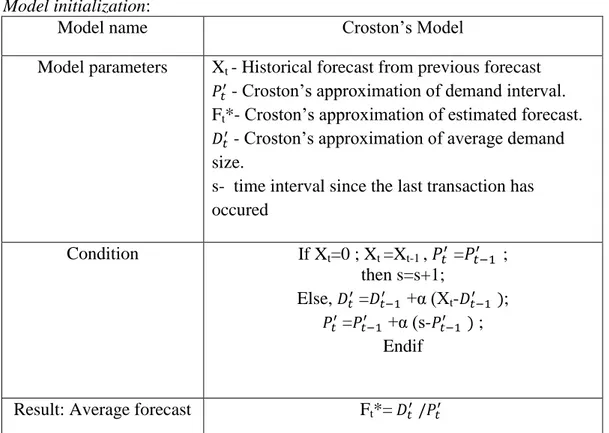
3.5 Croston’s method of forecasting
Inventory problem dealing with products of irregular or lumpy demand is a common issue. Those products with the lumpy demand mainly include high cost components such as engines, axles, frames, dumpers or heavy machinery equipment etc. Improving forecast accuracy for these products with lumpy demand is the most important challenge in the inventory management (Vasumathi & Saradha, 2013).
Croston (1972) built a forecasting model for the products that have intermittence in their demand. He decomposed this method into parts, i.e. to measure the time interval between the demand periods and to calculate the forecast value when there existed a demand. Later on various authors such as Willemain et al (2004), Wallström & Segerstedt (2010), Synetos & Boylan (2005) etc. have clarified this method and have examined by applying the real
20
industrial data and have achieved incredible results. Few authors have modified it to some extent based on their findings from the past researches and achieved appreciable results. Croston’s method of forecasting is one of the best practices applicable for the products with intermittent or sporadic demand. Croston’s method was built mainly to establish accurateness to calculate mean demand over a time period (Willemain et al 2004).
Willemain et al (1994) had conducted a comparison study of Croston’s forecasting method with the exponential smoothing method in two different ways. Firstly, using the Monte-Carlo comparison he tried to build the algorithms in order to deviate from the assumptions made in Croston’s method with respect to the probability distribution. And secondly, by using industrial data from three to four different companies he tried to measure the forecast accuracy and compared it.
It was seen that the exponential smoothing method was most commonly used for inventory control of high volume products, but at times it can end up in the fluctuation in the stock levels (Willemain et al 1994). Croston’s method consist of two steps, first to estimate the average demand size by exponential smoothing and second to estimate the average time interval between the demand. According to Croston’s method the structure of demand is segmented into two factors, they are the meantime between the demand and the magnitude of the demand. The assumptions made in Croston’s method are the demand pattern follows the Bernoulli distribution and the size of the demand was assumed to have a normal distribution. The equation for average demand size and average meantime between demands is expressed as, If Xt=0, 𝐷𝑡 ′ = 𝐷 𝑡−1 ′ 𝑃𝑡 ′ = 𝑃 𝑡−1 ′ s = s+1 Else, 𝐷𝑡 ′ =𝐷 𝑡−1 ′ +α (Xt - 𝐷𝑡−1 ′ )………(1) 𝑃𝑡 ′ =𝑃𝑡−1 ′ +α (s-𝑃𝑡−1 ′ )……….(2) (Willemain et al., 2004, pp.379)
Where, Xt is the historical forecast from previous forecast, s- time difference between the
two latest period with demand, 𝐷𝑡 ′ is Croston’s approximation of average demand size, 𝑃 𝑡 ′
is Croston’s approximation of average meantime between demand, α- smoothing factor (ibid).
By combing the above two computed values, the estimated mean demand per period is calculated as,
Ft* = 𝐷𝑡 ′ /𝑃𝑡 ′ ………. (3) (Willemain et al., 2004, pp.379)
3.6 Improving Forecast performance and accuracy
According to (Jacob et al., 1999), in order to achieve higher forecast accuracy it is essential to consider some important aspects. At times forecasting gets complicated and it will be hard to understand, in such instances the organization needs to consider that every individual working on forecasting has a different level of understanding. Hence in order to improve the forecasting performance level, it is pretty clear that the employee’s working on forecast get expertise from their work experience and knowledge from their workplace. Mainly by studying the earlier years forecasting patterns and having understood the past forecast errors it is possible to identify the necessary measures that can be solved and developed for the future forecast. (ibid)
21
According to Liker & Meier (2006), in this competitive world to be more efficient in the business area it is essential to have sound knowledge and proper guidelines or meet the company standards. The guidelines are normally built by adopting documentation; it is a set of instructions which gives a clear picture of the how the given task has to be executed. It is mentioned that without building a clear structure it is impossible to figure out the possible improvements (ibid).
According to Mentzer (2004), it is essential for every team member who works with forecasting to get personal feedback of their job performance. So that they get to know their area of improvement in order to improve the forecast accuracy. Moreover, it is also essential for them to know the negative impacts of poor forecast as it can hampers the whole loop such as inventory, capacity planning, production etc. Hence the author also stresses on the fact that, it is really important for the employees to perceive the purpose of forecasting who are working on it. They should understand how the footprint made by forecasting on the company and their customers. Also, the author makes a final note that, in order to succeed with improved forecast accuracy it is really essential to give training to the employees to improve the performance for those working with the forecast. By providing good qualitative training to the employees it is possible to improve the company’s forecast accuracy. (ibid)
3.7 Strategic Resource Planning (SRP)
The purpose of Strategic Resource Planning (SRP) is to predict the demand of a company’s products and services for an extended period of time, and planning the resource allocation in order to execute it in the most optimal way. According to Vancil & Lorange (1975) “Strategic resource planning (SRP) is defined as the process of gradual tapering of the tactical options that are intended to be fulfilled over the coming time period”. (ibid)
In the SRP driven forecast, there will be good blend of the market input and some speculations involved in the planning stage (Bucklin, 1965). In most of the profitable organizations, their key to success is knotted by effectively linking the forecast and the allocation of resources in an optimal way (Wacker & Lummus, 2002). The resources are determined by three main factors they are availability, capacity and location. These three parameters are the driving factors of the SRP system. In order to establish a successful resource plan, the planning is done in three stages and they are strategic, tactical and operational. It is shown in figure 9 (Owusu, et al., 2008).
These three core components of resource planning are interlinked and they communicate by sharing data between them. The figure below shows the relationship among the core components of resource planning.
22
Figure 9: Flow of information between the three levels of planning (Owusu, et al., 2008, p.36) Shaw et al., (1998) have mentioned that SRP is a tool that can be regarded as a process of review of various critical factors for success. SRP is a logical connecting process which requires two important ingredients and they are large number of investors and different sources to gather information such as market inputs from customer centers, macroeconomic data etc. There should be a good flow of information and coordination among the investors (Owusu, et al., 2008). When there is good coordination and true information is exchanged among the investors then it is a sign of making a successful strategic plan in any organization.
3.7.1 Importance of sales forecasting for Strategic Resource Planning (SRP)
The sales forecasting is a sub area under business forecasting (Armstrong, 1985). It is a process of predicting the future business sales that the organization intends to obtain. The sales forecast can be estimated on yearly, quarterly or monthly basis. Sales forecasting plays a crucial role in estimating the future demand, doing long term production planning of upcoming sales and to allocate the resources in an optimal way (ibid).
It is clear that for any manufacturing organization without the bond between forecasting and resource allocation it is not possible to gather enough resources in order to make delivery on right time to the customers (Wacker & Lummus, 2002). And the author also highlights that the role of sales forecast is really crucial, since it gives information about the future demand and based on that it is possible to build long term production planning. To be more precise, storing the right products to meet the sales is impossible without any pre-sales forecast. While implementing strategic thinking it is clear that company’s success relies on efficiency of the bonding between resource planning and forecasting. Strategic resource planning is done with the purpose that it reduces the forecast error which was obtained from the sales input (ibid).
3.8 Inventory management
The inventory management system focuses on three main aspects they are: How often the replenishment needs to be done, size of the replenishment order and how often the inventory status has to be reviewed (Silver 1981; Chatfield & Havya 2007).
Strategic Operational