Design and Development of an Experimental Test Rig for Heat Sinks

(1)

IN

DEGREE PROJECT INDUSTRIAL ENGINEERING AND MANAGEMENT,

SECOND CYCLE, 30 CREDITS ,

STOCKHOLM SWEDEN 2020

Design and Development of an

Experimental Test Rig for Heat

Sinks

GABRIEL KADUVINAL ABRAHAM

KTH ROYAL INSTITUTE OF TECHNOLOGY

(2)

TRITA ITM-EX 2020:549

(3)

1

Sammanfattning

Värmesänkor, som exempelvis kylflänsar, används främst för att transportera bort värme som orsakas av förluster i en komponent. Denna värmeöverföring möjliggör en smidig drift av systemet där den värmegenererande komponenten ingår. Värmesänkans effektivitet beror på hur mycket värmeeffekt den kan transportera bort. Flera olika konstruktioner och tillverkningstekniker har utvecklats för att förbättra värmesänkors kylprestanda.

Målet med detta projekt är att bygga en testrigg som kan användas för att testa kylflän-sars effektivitet. Testriggen ska utformas så att den är modulär, dvs. den ska kunna användas för att testa kylflänsar av olika storlekar. Projektet startade med en bred in-formationssökning om kylflänsar och olika testmetoder. En systemarkitektur skapades som ett början och för att hitta systemets olika principkomponenter. De viktigaste huvudkomponenterna som uppfyllde designkraven valdes sedan. En kylare med pump, en flödesmätare med regulator, temperatur- och tryckgivare och rörledningar, inklu-sive ett flexibelt rör var de viktigaste komponenterna i det system som skapades. De specifika komponenterna valdes sedan och de representerades och arrangerades på ett kompakt sätt som en system-CAD-modell i SolidEdge. Efter flera iterationer valdes en slutlig konstruktion, och den experimentella testriggen byggdes sedan i flödeslab-oratoriet. Den experimentella testriggen kan justeras för att installera kylflänsar av olika storlekar, vilket innebär att den, i viss mån, är modulär. Framtida arbeten för att förbättra testriggens prestanda föreslås också.

Nyckelord: Kylning, experimentell installation, flödeshastighet, kylfläns, VVS, sen-sorer, värmeeffektivitet.

(4)

(5)

3

Abstract

Heat sinks are used mainly to take away the excessive heat which are produced in a component. This transfer of heat enables a smooth operation of the system with the heat generating component. The efficiency of heat sink is often dependent on the amount of heat it can take away within the smallest duration of time. Several designs and manufacturing techniques have been developed to improve this performance of heat sinks.

This project aims at building a test rig which can be used to test the efficiency of heat sinks. The test rig should be designed to be modular, i.e. it should be able to test heat sinks of different sizes and also adhering to the design requirements. The project started with a broad information search on heat sinks and different testing methods. A system architecture was formulated for this test rig as a beginning stage and to find the different architectural components. The main principal components were selected fulfilling the design requirements. A chiller with pump, a flow meter with controller, temperature and pressure sensors and piping’s including a flexible pipe were the main components of the system created. When the specific components were chosen, the design was embodied and the components were arranged in a compact manner as a SolidEdge CAD-model. After several design iterations, a final design was selected. The experimental test rig was then built in the flow lab. The built experimental test setup is able to be adjusted to install heat sinks of different sizes making it modular in design. Future work to improve the performance of the test rig is also suggested. Keyword: Cooling, Experimental Setup, Flow rate, Heat sink, Plumbing, Sensors, Thermal Efficiency

(6)

(7)

5

Foreword

I would like to express my gratitude to Rebei Bel Fdhila and Manoj Pradhan from ABB Power Grids, who was the industrial supervisor and manager providing me with all the support I needed during the whole project. Their guidance on selecting and assembling was significantly useful that helped this project come true.

I would also like to take this opportunity to express my profound and sincere gratitude, indebtedness and affinity to my respected guide Prof. Ulf Sellgren for his professional guidance, valuable advises, constructive criticism and immense help throughout the course of the project work.

I also thank Tjorborn Wass, Saeed and Lokman Hosain from ABB PGR for the help they have provided me with the designing and selection phase of my project.

Above all, I thank God Almighty without whose blessings my efforts would not have been a reality.

Gabriel Kaduvinal Abrahaml Västerås, 30-09-2020

(8)

(9)

7

Nomenclature

Notations

A Area of cross section (m^2) Aprime Area of heat sink base

c Specific Heat (J/kg.K) cp Specific Heat (J/kg.K)

g Acceleration due to gravity (m/s) h Elevation (m)

˙h Heat transfer coefficient l Length of the pipe (m) m Mass (kg)

˙

m Mass flow rate (L/min)

Ploss Total power loss from one side (kW)

p Pressure (Pa) Q Heat Transfer (J)

q Volume flow rate (m^3/s) Rth Thermal Resistance (K/kW)

r Radius of the pipe (m) ∆T Change in Temperature (K)

Tavg,subM Average temperature of submodules’ surfaces (°C)

Tavg,f luid Average fluid temperature of inlets and outlets (°C)

Tout Temperature at the outlet (°C)

Tin Temperature at the inlet (°C)

Ts Temperature of the heat sink substrate (°C)

V Velocity (m/s)

(10)

(11)

9

Nomenclature

Abbreviations

ABB ASEA Brown Boveri AM Additive Manufacturing

BIGT Bimode Insulated Gate Transistor CAD Computer Aided Design

CFD Computational Fluid Dynamics HVDC High Voltage Direct Current

(12)

(13)

Sammanfattning 1 Abstract 3 Foreword 5 Nomenclature 7 Table of Contents 11 1 Introduction 17 1.1 Background . . . 18 1.2 Purpose . . . 18 1.3 Delimitations . . . 19 1.4 Methodology . . . 19 2 Project Planning 21 2.1 Requirement Specification . . . 21 2.1.1 Performance . . . 21 2.1.2 Environment . . . 21

2.1.3 Target Product Cost . . . 22

2.1.4 Safety . . . 22

2.1.5 Legal . . . 22

2.1.6 Materials . . . 22

2.1.7 Aesthetic and Appearance . . . 22

2.1.8 Installation . . . 22 2.1.9 Life in service . . . 22 2.1.10 Time scale . . . 23 2.1.11 Maintenance . . . 23 2.2 GANTT-Chart . . . 23 11

(14)

Contents 12

3 Frame of Reference 24

3.1 Heat Sinks . . . 24

3.2 Principle of heat sinks . . . 25

3.3 Design Parameters of Heat Sink . . . 26

3.3.1 Material . . . 26

3.3.2 Thermal Resistance . . . 26

3.3.3 Fin Efficiency . . . 27

3.3.4 Fin Arrangement . . . 27

3.4 Methods to determine performance of a Heat Sink . . . 27

3.4.1 Numerical Method . . . 28

3.4.2 Experimental Setup . . . 28

3.5 Heat Sinks in HVDC application . . . 30

3.6 Parameters Affecting the Test Rig Design . . . 31

3.6.1 Mass Flow Rate, Velocity of Flow and Cross-sectional area of piping . . . 31

3.6.2 Bernoulli’s Equation . . . 31

3.7 Existing Temporary Test Rig in Flow Lab . . . 32

4 Implementation 34 4.1 Architecture Definition . . . 34

4.1.1 Cooling unit and Reservoir (Chiller) . . . 35

4.1.2 Pump . . . 36

4.1.3 Flow Meter . . . 37

4.1.4 Sensors . . . 37

4.2 Component Selection . . . 38

4.2.1 Integrated Chiller with Reservoir and Pump . . . 38

4.2.2 By-Pass Piping . . . 44

4.2.3 Flow Meter with Integrated Flow Controller . . . 45

4.2.4 Flow meter MID DN25 . . . 47

4.2.5 Temperature Sensors . . . 48

4.2.6 Pressure Sensors . . . 49

4.2.7 Piping, Connectors and Insulation . . . 50

4.3 Working . . . 52

5 Results 53 5.1 Preliminary and Final Design . . . 53

6 Discussions and Conclusion 59 6.1 Discussion . . . 59

(15)

13 Contents

7 Recommendations and Future Work 61

References 62

Appendices 64

A Risk Table A

B Specifications B

(16)

List of Figures

2.1 Gannt chart of the whole project . . . 23

3.1 Heat Sinks . . . 25

3.2 Fourier’s Law of heat conduction . . . 26

3.3 Thermal profile on a heat sink . . . 28

3.4 Heat sink Test Apparatus . . . 29

3.5 Bernoulli’s Principle . . . 32

4.1 Pictorial demonstration of the test rig (FC and S denotes the flow meter and controller and the sensors) . . . 35

4.2 Recirculating cooler FL7006 . . . 38

4.3 Plot showing pump capacity at different pressures . . . 39

4.4 Recirculating cooler FL1203 . . . 40

4.5 Plot showing pump capacity at different pressures . . . 41

4.6 Thermo Chiller HRS 050-AF-20 . . . 42

4.7 Working of Thermo Chiller HRS 050-AF-20 . . . 43

4.8 By-Pass Piping set . . . 45

4.9 Digital Flow Sitch PF3W740S-F06-BN-M . . . 45

4.10 Variation Chart of Flow meter . . . 46

4.11 Flow meter MID DN25 . . . 47

4.12 RT-B-BP1 (Compact temperature sensor) . . . 48

4.13 Ceramic Pressure Sensor . . . 49

4.14 Sensor Holder . . . 50

4.15 Pipe insulation . . . 51

5.1 Preliminary Design in top view . . . 54

5.2 Preliminary Design in isometric view . . . 55

5.3 Final Design in top view . . . 56

5.4 Final Design in isometric view . . . 56

5.5 Experimental Setup Front View . . . 57

5.6 Experimental Setup Side View . . . 57

(17)

15 List of Figures

6.1 System architecture made on SolidEdge . . . 60 A.1 Risk Analysis Table . . . A B.1 HRS-050-AF-40 Chiller specifications . . . B B.2 Flow switch PF3W740S-F06-BN-M Specifications . . . C C.1 Main Assembly draft . . . D C.2 Chiller Draft . . . E C.3 Flow meter draft . . . E C.4 Sensor holder draft . . . F C.5 Copper pipe draft . . . F C.6 Table draft . . . G

(18)

(19)

Chapter 1 Introduction

Excessive temperature is one of the main causes of failure for most of the microelec-tronics. Heat exchangers have been used from the old ages itself for the efficient cooling or heat removal purposes in electrical or mechanical devices, keeping the temperature of the system at optimum level. Heat exchangers uses either air cooling or water or certain fluids to take away the heat from the system. When water is used as a medium to remove heat through the heat sink it’s called as a cold plate. The electronic indus-try is constantly working on miniaturization and functional integration and thereby increasing the heat produced in these electronic components. The heat dissipation ca-pability of electrical components itself might not be enough to keep the temperature at moderate levels. This is where the heat sinks, or cold plates are useful to achieve a de-sired temperature by transferring heat from the component to the environment. Heat sinks are usually modelled with maximized contact area with materials having high heat transfer properties like aluminium or copper. A heat sink works on the principle of Fourier’s law of heat conduction.

Cold plates are designed in a way with an inlet and an outlet on a geometry usually as a square or a rectangle. The inlet takes in the cold fluid into the plate, onto which the component to be cooled is placed, and leaves through the outlet which can be on the same side of the inlet or on the opposite side. The temperature of the outlet fluid will be higher than the inlet due to the heat it had absorbed from the component. This fluid will be then sent to a reservoir where the temperature will be kept constant. In recent days, works are done on the shapes and profiles of the pipes in heat sinks to increase its efficiency in carrying away the heat. Studies have been done on using Additive Manufacturing (AM) to produce cooling channels in heat sinks for High Voltage Direct Current (HVDC) Bimode Insulated Gate Transistor (BIGT) units. This has brought a huge difference in the manufacturing industry and in the performance in the heat exchanger sector.

(20)

Chapter 1. Introduction 18

This thesis work focuses on building a test rig to test the efficiency of different heat sinks which are designed and manufactured.

1.1 Background

ASEA Brown Boveri (ABB) is Swiss Swedish Multinational corporation based in Zurich. The company is mainly operating in Robotics, power, heavy electrical equipment and automation. This thesis work is done at the ABB Power Grid research within the department of Applied Physics. Power Electronics being one of the main divisions, research works are done on constant design improvement on heat sinks. With constant redesigning of the heat sinks, the need to test its efficiency also is of prime importance. The simulations are done on Computational Fluid Dynamics (CFD). These results are then validated with an experimental setup which is built in the fluid lab at ABB. The experimental setup used for the testing of heat sinks had variety of components like a cooling unit, a reservoir, a pump to pump the fluid throughout the system and also temperature and pressure sensors for the measurements. The sensors used in this temporary setup were not of high precision or accurate and also the ranges were not quite defined. The experimental setup was also build just for a predefined, heat sink dimension. This made it difficult for the testing of heat sink with different sizes. Moreover, the test rig was built from scratch every time they need to do a test on a new heat sink, making it difficult and time consuming.

1.2 Purpose

Testing of the heat sinks/cold plates experimentally and validating it with the results through numerical approach such as Computational Fluid Dynamics (CFD) before active usage in the industry is of prime importance. This can be achieved by testing the cold plate on a test rig which is already set up with a pump, temperature controlling reservoir, temperature and pressure sensors and a flow control unit.

The main aim of this thesis work focuses to the design and development of a compact and modular test rig which can be placed in the heat and fluid lab in ABB. This means the components on the rig should be easily disassembled and should stay stable for quite several tests. The cold plate should be able to be easily installed onto the test rig and tested with the least work. The test rig includes a pump, a temperature control reservoir, a flow control unit, temperature and pressure sensors. A data acquisition system will be used to read and evaluate the results.

The test rig also should be able to take heat sinks of different dimensions making it flexible and modular for different heat sink designs. The temporary rig which exists can

(21)

19 1.3. Delimitations

be only used to do testing on a heat sink or cold plate of a pre-defined dimension. This made it expensive for testing and also time consuming for testing of different design heat sinks. The thesis work mainly aims on designing a test rig which can accommodate a range of heat sinks with different dimensions and also the pressure range should be with in a certain range to ensure safe testing of these heat sinks.

Research Question

a) What will be the preferred architecture for the test rig? b) What are the main components on the experimental setup?

1.3 Delimitations

a) In depth study of heat sinks are avoided and necessary values for the calculations are taken from the existing internal reports on heat sinks using CFD.

b) CFD simulations and design on the heat sinks are not included in the thesis work. c) Installation design of the heat sinks are not considered on the test rig and this is

taken as a black box.

d) Testing is out of scope for the project because of the lack of time. e) There was a budget restriction for the total test rig.

1.4 Methodology

a) Background Study and Literature Review

i) Basic working principles of a heat exchanger.

ii) Internal reports on CFD simulations done on heat sinks and thorough under-standing of the results from it.

iii) Detail study of temporary design in the fluid lab at ABB.

iv) Factory visit at Ludvika to study the large-scale heat exchanger rigs. b) Identification of design parameters on the whole test rig.

c) Identification of different components of the experimental setup. d) Concept generation.

(22)

Chapter 1. Introduction 20

f) Budget presentation

g) Design Selection and verification. h) Building the test rig.

(23)

Chapter 2 Project Planning

2.1 Requirement Specification

2.1.1 Performance

The final design should meet the following requirements: a) The flow should be able to be controlled from 0 to 25 l/min b) Constant supply of input power of 4kW

c) Maximum pressure difference of 2 bars between the heat sinks d) Fluid such as water glycol mixture can be used.

e) Velocity of the fluid is 2 m/s.

f) Testing of heat sinks of different sizes should be possible.

2.1.2 Environment

a) Noise level: below 80-85 db. This is desired for the safe working environment of the personnel;

b) No corrosion from the working fluid. Desired to avoid any form of degradation of the materials used;

c) Environment friendly components. Desired to avoid dangerous products and risks following them;

d) Personnel Safety;

(24)

Chapter 2. Project Planning 22

e) Use of non-hazardous materials. Desired for the health of personnel in contact with the prototype.

f) Avoid spillage of the working fluid used in the design.

2.1.3 Target Product Cost

A budget of 70,000 SEK was approved for the project after the component selection during the budget presentation

2.1.4 Safety

a) Should comply with EU workplace standards on Physical, chemical and electrical safety;

b) Personnel safety should be taken into account; c) Use of non-hazardous materials.

2.1.5 Legal

The product should meet the Consumer Protection Policy.

2.1.6 Materials

a) Materials selected were mostly copper pipings and plumbing parts. b) Non-hazardous and should comply with EU environmental standards.

2.1.7 Aesthetic and Appearance

Austere and Ergonomic design.

2.1.8 Installation

a) Easy installation; b) Good modularity;

c) Effortless changing of working fluid.

2.1.9 Life in service

(25)

23 2.2. GANTT-Chart

2.1.10 Time scale

a) Rig development by July end.

2.1.11 Maintenance

Easy Maintenance.

2.2 GANTT-Chart

GANTT chart is a bar chart that defines a project schedule from start to finish. The chart that was used for the concept generation and evaluation phase is shown below in Figure 2.1.

(26)

Chapter 3 Frame of Reference

This section explains topics which helped to be the backbone and basics of this thesis work. The chapter explains the general topics related to the project. It also describes about the existing work which was available at the lab but with limited details due to confidential reasons.

3.1 Heat Sinks

A heat sink is usually used as a medium to dissipate heat from a mechanical or elec-trical working component thereby keeping the working temperature of the component regulated. The heat sinks uses either air or liquid as a working fluid in it. Its commonly called as a cold plate when the fluid used in the heat sink is liquid. This can be of different properties depending on the purpose and surroundings. Most of the time it will be water or water glycol mixture due to its high specific heat capacity property. They are usually used when the heat dissipation property of the component itself is very poor. The most commonly used places are in CPU’s, RAM modules and chip sets. They are also often seen in diodes and power transistors.

(27)

25 3.2. Principle of heat sinks

Figure 3.1: Heat Sinks

Figure 3.1 shows some of the heat sink designs that are used in the electronic industry. The design and the area of contact of the heat sink with the component plays a major role in the performance of the heat sinks and the amount of heat it can take away from the component. There are usually several treatments done on the heat sink and also the material selection which can improve the performance of the heat sink. Also the contact between the device and the heat sinks are filled with some thermal insulators or adhesives for the maximum contact and less heat transfer to the surrounding air. Copper and Aluminum are the most commonly used heat sink material.

3.2 Principle of heat sinks

The power supply on any electronic are not always completely efficient. In situations like these, there is chance of extra heat production on the component which can cause problems with the working. Heat sinks are used for instances like this. The heat energy is usually transferred from a higher temperature to a lower temperature. The lower temperature is here maintained with the fluid in the heat sink. The fluids are often used as air, water, oil or any refrigerants. In thermodynamics, heat sinks are often described as reservoirs that can absorb random amount of heat without much increase in the overall temperature of the heat sink. The mode of heat transfer on heat sinks can be either conduction, convection or radiation.

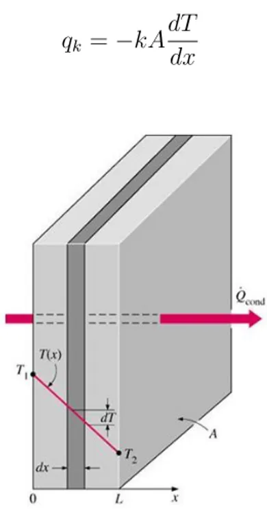
Heat sinks works on the principle of Fourier’s law of heat conduction. This law explains that if there is presence of a temperature gradient in a body, there will be heat transfer from a higher temperature region to a lower one. Fourier’s law states that the rate of heat transfer by conduction is proportional to the temperature gradient and the cross

(28)

Chapter 3. Frame of Reference 26

sectional area of the heat transfer region.

qk= −kA

dT

dx (3.1)

Figure 3.2: Fourier’s Law of heat conduction

3.3 Design Parameters of Heat Sink

3.3.1 Material

The most common materials used to make the heat sink or cold plates are either aluminium or copper. Aluminium is more widely used than copper because of its lower price compared to aluminium, even though copper has almost twice the thermal conductivity than aluminium. Copper is extremely denser and more expensive than aluminium. Aluminium alloys are the most often used heat sink material. They are usually made using process like casting, milling or extrusions.

3.3.2 Thermal Resistance

The efficiency of a heat sink or a cold plate is often decided by the factor thermal resistance. Heat sinks are mostly selected after calculating its thermal resistance since it helps to give an idea of how small or big the resistance value is thus giving you an approximation of how much heat it will be able to take off at a given time. Heat sinks of low thermal resistance are mostly preferred because this shows the heat can be taken away in bigger quantities when the resistance is less.

(29)

27 3.4. Methods to determine performance of a Heat Sink

This thesis work also aims at building a test rig which will be used to measure the thermal resistance of different heat sinks thereby helping to evaluate and validate dif-ferent heat sink designs with the fluid simulations done on ANSYS. Thermal resistance is defined as the rise of temperature per unit power, expressed in (K/kW).

3.3.3 Fin Efficiency

Fins are part of the heat sinks which are projected from the base and are usually flat plates. Fin materials are selected considering the conductivity factor. A high thermal conductivity helps the heat to flow easily and at the maximum rate. A fin efficiency is defined as the actual heat transferred by the fin of the heat sink to the heat transferred by the fin considering the fin to have an infinite thermal conductivity.

3.3.4 Fin Arrangement

The arrangement and design of the fins on the heat sink is what makes the efficiency better or worse. Designers in the field of heat sink design keep improving the design of fins everyday to provide a heat sink having the best heat removing properties. The fins decides on factors like how fast it can take the heat through it from the surface to the surrounding environment. Fins can be of different designs. The most common used fin design is the pin design where they pack pin shaped long fins on the heat sink. The shapes of the pin can be either square, elliptical or cylindrical.

3.4 Methods to determine performance of a Heat Sink

The performance of a heat sink depends on factors like thermal resistance, thermal conductivity, material of the heat sink, size of the heat sink, area in contact, type of fin used on the heat sink, heat transfer coefficient and also the fluid flow rate on the heat sink.

The thermal performance of a heat sink can be found using theoretical as well as experimental or numerical methods. This thesis being completely focusing on an ex-perimental setup to determine the thermal resistance of different heat sinks. Since the flow in the heat sinks are considered to be complex in nature, these are usually calculated in Computational Fluid Dynamics (CFD) simulations.

This thesis work mainly focuses on the experimental and the numerical methods. The results from the numerical method is used to validate the results that are obtained from the experimental setup.

(30)

3.4.1 Numerical Method

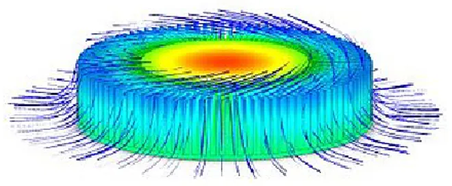
CFD simulations are done in the design phase of a heat sink which helps to give an approximate performance before the heat sinks are made physically. But often this is ignored which makes the redesigning expensive and hard. CFD simulations can give both qualitative and quantitative result of the flow of the fluid in heat sinks. It can give the visual results on the heat flow through heat sinks. The accuracy of these results depend on the parameters which were given as input through the software. The main advantages of the numerical method over the experimental way of determining the performance is that simulations can be done for different parameters at the same time and also keeping it inexpensive. The flow rates which are difficult or impossible can be also carried out in numerical simulations.

Figure 3.3: Thermal profile on a heat sink

The figure 3.3 above shows the thermal profiles on a random heat sink which was done on a CFD simulation.

3.4.2 Experimental Setup

Once the numerical simulation is done on a heat sink, it is most of the time compared with a experimental test. Physical tests on the heat sinks are the most popular way to determine its thermal performance. These tests are done on test rigs which can give you multiple measurements. The thermal resistance is usually the parameter determined from the test which in turn gives the thermal performance of the heat sink. Factors like the flow rate of fluid, inlet temperature of the fluid, input power provided and base temperature of the heat sink need to be known to calculate the thermal resistance from the setup. The experimental test results depend on environmental factors and for this reason the test rig are usually insulated or ducted.

(31)

29 3.4. Methods to determine performance of a Heat Sink

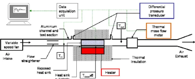
Figure 3.4: Heat sink Test Apparatus

Figure 3.4 shows a test apparatus which was build to study the pressure loss and the heat transfer through heat sinks by a research team of M.Wong, I.Owen and C.J.Sutcliffe [8]. The test setup uses air as the fluid and consists of an inlet and outlet and a flow straightener promising a steady and straight flow in the system. There are temperature and pressure measurement units at both the inlet and the outlet.A blower is used to give constant supply of air into the system and also the flow rate can be controlled. The input power is controlled by controlling the input voltage to the heater.The heater and heat sink is completely insulated for avoiding any form of heat loss in the system and to give a better result. The base temperature of the heat sink is calculated by taking an average of all the six thermocouple measurements situated in the substrate of the heat sink. The measurements are continuously fed into the data acquisition system for plotting and reading purpose.

The heat sink to be tested is placed on the heater as shown in fig 3.4. An input power of certain value in kW will be continuously supplied to the heat sink. The fluid which is air in this setup will be blown from the fan. This air takes away a certain amount of heat from the heat sink along with it when it passes through it. The amount of heat and the efficiency of this depends on the heat sink profile and the fins provided on the heat sink. The temperature before and after the heat sink is measured for the calculation purposes. The pressure difference between the heat sink is also a major parameter that needs to be measured. This is measured using the differential transducer shown in the figure. A mass flow meter is also used for the precise mass flow rate readings from the experimental setup.

The heat sinks performance is often considered after studying how much heat it can dissipate from the surface of the heat sink. The heat transfer performance is measured

(32)

from calculation the heat transfer coefficient ˙h. ˙h = mc˙ p(Tout− Tin)

Aprime(Ts− Tα) (3.2)

where, ˙

mis the mass flow rate of the fluid in the experiment setup you measure from the flow meter.

cp is the specific heat of the fluid considered.

Tout, Tin, Ts, Tα are the temperatures at the outlet of the heat sink, inlet of the heat

sink, heat sink substrate.

Aprime is the area of the heat sink base.

After the heat transfer coefficient is calculated, these values are compared and validated with the simulation results from software.

This thesis work focuses on designing and building an experimental test setup for testing different heat sinks similar to this, with changes such as using water or water gycol mixture as the fluid and changes related to that. The main challenge in this is to select the components for the test rig which matches for the different parameters and specifications.

3.5 Heat Sinks in HVDC application

The demand of electric current has been booming recently in the industrial applica-tions. In result to this miniaturization of high voltage direct current (HVDC) converter devices are increasing as well. The miniaturization of these HVDC converters to convert alternative current (AC) to direct current (DC) in high power transmission systems in turn gives out the problem of increased heat flux produced in this system. This can sum up to a 30 percent of the total power loss in the HVDC device. In high dissipation cases like these, the insulated gate bipolar transistor IGBT which is highly sensitive, faces the problem of thermal runaway. This is because silicon cannot be used at such critical thermal conditions. This can be sometimes solved by using an alternative mate-rial for silicon and does not completely solve the problem all throughout. For instances like these, heat sinks are the best solution for managing the thermal conditions in the system. To fit the heat sink to the small size HVDC units, the heat sinks are also made smaller in size these days which makes it challenging to provide an efficient and advanced cooling solution.

(33)

31 3.6. Parameters Affecting the Test Rig Design

3.6 Parameters Affecting the Test Rig Design

3.6.1 Mass Flow Rate, Velocity of Flow and Cross-sectional

area of piping

Q = AV (3.3)

Equation 3.2 shows the flow rate formula which connects the flow rate, area of cross section and the velocity of the flow. Here Q is the volume flow rate in m3_/sor L/s, A

is the area of cross section in m2 _{and V is the velocity of the flow in m/s.}

The mass flow rate and the velocity of the fluid is given as a design specification and thus the area of the pipes which are used for the test rig are found using this.

˙

m = ρAV (3.4)

Equation 3.2 can be rewritten as shown in equation 3.3 in terms of mass flow rate, density of the fluid, area of cross section and velocity of the flow.

This equation is primarily used to calculate the mass flow rate of the fluid needed at the pump. Here the density is taken as 1000kg/m3 _{(density of water), area for the heat}

sink is taken from the existing design and already known velocity of the flow.

3.6.2 Bernoulli’s Equation

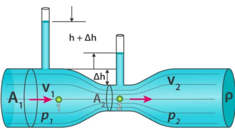
The Bernoulli’s equation is used to calculate any sort of pressure buildup or differences in the whole test rig at any point or connections. The equation states that,

p + 1 2ρV

2 _{+ ρgh = constant} _(3.5)

where p is the pressure, ρ is the density, V is the velocity, h is the elevation and g is the acceleration of gravity. The equation explains the energy conversion happening in a fluid system between pressure, velocity and elevation for a continuous flow.

(34)

Figure 3.5: Bernoulli’s Principle

In case of pipes of different cross section the equation changes to,

p1 + 1 2ρV 2 1 + ρgh1 = p2+ 1 2ρV 2 2 + ρgh2 (3.6)

where suffices 1 and 2 corresponds to the two areas in the piping. The equation is also used for calculation of static pressure in the system as well.

When the streamline is considered to be parallel and the gravity is ignored, the equation would become, p1− p2 = 1 2ρ(V 2 2 − V12) (3.7)

3.7 Existing Temporary Test Rig in Flow Lab

A test rig was used in the flow lab in ABB PGR in Vasteras for testing the performance of heat sinks. This setup was though a temporary fixture and was disassembled and moved away after every single testing like explained in the beginning sections.The details regarding this test rig is disallowed to be explained due to confidential reasons. This section explains an overview of the temporary test rig which was used. The test rig included pipes which were directly connected to the tap water. A flow meter was installed on the way to the heat sink before the sensors. The flow meter was the main source of flow rate reading since the flow was directly taken from the tap. The heat sink had sensors, both temperature and pressure sensors on either side which gave the

(35)

33 3.7. Existing Temporary Test Rig in Flow Lab

measurements of inlet and outlet temperature and pressure. The water after exiting the heat sink was taken out to a sink continuously. The main disadvantage of this test rig being that it took time for the temperature of the flow to be constant since it was directly from the tap. This also give an ambiguous measurements for the temperature. Also the flow rate of the fluid was difficult to be controlled.

On an overview the measurements were not exactly accurate and had many difficulties in controlling the whole system. As explained before the test rig was built just to test a heat sink of a certain fixed dimension making the testing limited to a single dimension heat sinks.

The thermal resistance was calculated by taking the temperature measurements from the sensors and also taking the average base temperature from the heat sink which was measured using thermocouples.

Rth=

(Tavg,subM − Tavg,f luid)

Ploss

, (3.8)

where,

Tavg,subM - Average temperature of submodules’ surfaces (°C).

Tavg,f luid - Average fluid temperature of inlets and outlets (°C)

(36)

Chapter 4 Implementation

This sections explains how the project was carried out from the stage of studying the different components of the test rig through system architecture, the proper selection of them by taking the design parameters into consideration and a final working of the overall design.

4.1 Architecture Definition

Building a test rig, one of the main tasks is to find the best components which suite to the design specifications and provide all the necessary measurements and readings without any fail. This project being highly dependent on precise measurement of temperature on the outlet and inlet of the heat sinks, we had to select the best sensors they had in the market. The main components that needed to build the test rig were: a) Reservoir for storing water/water-glycol mixture,

b) Cooling unit (Preferably same unit with the reservoir), c) Pump with a pressure head of at least 3 bar,

d) Flow meter with controller, e) Pressure and temperature sensor, f) Piping’s and other fittings.

A small demonstration of how the test rig would look like is shown below here,

(37)

35 4.1. Architecture Definition

Figure 4.1: Pictorial demonstration of the test rig (FC and S denotes the flow meter and controller and the sensors)

This report mainly discusses on the main two design of component selection out of the many which was designed depending on the size, compactness, budget and the design specifications.

The flow rate of the system was first decided to be 43L/min which was taken from an internal report in the company and was later changed to 23L/min with the design update of the heat sinks and business. This was one of the main changes in the design that took place later in the project which helped choose the perfect pump which helped the test rig stay within the budget.

4.1.1 Cooling unit and Reservoir (Chiller)

Cooling unit or the chiller acts a main role in the test rig since the system has to be maintained at a constant temperature throughout the test.The cooling unit has to take away a heat of almost as big at 4 kW which is constantly supplied from the isolated heating unit placed beneath the heat sink. So a chiller with a cooling capacity of more than 4 kW is suggested in this case. The chiller should be also powerful enough to do the same cooling at different flow rates from 5 to 23 L/min. Since the chiller here also acts as a reservoir for the whole system, it has also been considered to have a tank capacity to hold enough fluid for the complete circulation.

The cooling capacity of the chiller should be more than the heating load which is 4kW. The temperature rise in the system is calculated using the equation Q=mc∆ T. Considering values for mass flow rate as 23 L/min, specific heat of water as 4182 J/kg

(38)

Chapter 4. Implementation 36

K and heat load as 4kW, we get the temperature rise to be about 2 degree Celsius. This in turn means a chiller with a cooling capacity of at least 4 kW or more should be selected for the smooth operation of the system with constant temperature without any rise in temperature in the system from the predefined temperature.

4.1.2 Pump

The pump is another important unit that decides the mass flow rate for the system. The mass flow rate needed for the test rig is calculated from the different heat sinks that need to be tested. The values are taken from the already existing heat sink simulations that are done in ANSYS. Two different calculations are shown below depending on the size of the heat sink that need to be tested and the flow rate for the system is fixed according to it.

Input data of the first heat sink:

Channels cross section size: 13mm x 3mm Number of channels: 4

Inlet diameter: 20.8mm

Velocity within the channels: 1 to 2 m/s

Maximum flow rate when velocity within channel is 2m/s: 0.013 m x 0.003 m x 4 x 2 m/s x 1000 l/m3 _{x 60 s/min = 18.72 L/min}

Input data for the second heat sink: Channels cross section size: 13mm x 4mm Number of channels: 4

Inlet diameter: 20.8mm

Velocity within the channels: 1 to 2 m/s

Maximum flow rate when velocity within channel is 2m/s: 0.013m x 0.004m x 4 x 2m/s x 1000 l/m3 _{x 60 s/min = 24.96 L/min}

Comparing these two mass flow rates, the second flow rate keeps the extreme value for the flow rate to be 25 L/min for the system and a pump should be selected according to it.

The pump pressure is another factor that needed to be considered while selecting the right pump. The pressure difference between the heat sinks were found to be at the maximum of 0.25 MPa at a flow rate as big as 43 L/min. So the upper value for the pump pressure is kept at 0.4 (4 bar) Mpa considering other pressure rises in the system.

(39)

37 4.1. Architecture Definition

4.1.3 Flow Meter

A flow meter is as important as the chiller to measure the flow at which the system is operating at. A flow controller is also of much importance in this test rig since most of the cases the chiller will be supplying the flow at a constant flow rate. The flow rate has to be controlled and should be able to be reduced to different lower values. For this, a flow meter with an integrated option to control the flow is suggested. It has to be made sure that the flow meter should be able to take both the water and water glycol mixture.

4.1.4 Sensors

Sensors being the fundamental part of the test rig is of the highest priority while selection and calculation. The test rig mainly calculates the thermal resistance of the heat sink tested on the experimental setup. This means the sensors should be highly responsive and also should be accurate close to the decimal places for the precise measurement.

The test rig mainly focuses on two types of sensors which are the temperature and pressure sensors. The main criteria to be looked into while selecting the temperature sensor are the accuracy, the tolerance range and the reaction time. Since all these factors affects the accuracy of the measurement, the final thermal resistance depends on them.

There will be two similar temperature sensors on either side of the heat sinks on the test rig. The temperature of the flow before and after the heat sink are measured. This is later used for the calculation of the thermal resistance using the equation,

Rth=

Ploss

, (4.1)

Ploss - Total power loss (kW)

While selecting the pressure sensor, the pressure sensor is of main importance. Because, in most of the cases, the accuracy of the pressure sensor depends on the full scale range of the sensors. So this should be taken into consideration while the selection process. In the case of pressure sensors also, we use two of them at the inlet and outlet of the heat sink for measurements. The pressure difference is calculated from these measurements during the testing.

(40)

4.2 Component Selection

4.2.1 Integrated Chiller with Reservoir and Pump

As discussed before the Chillers were studied with different flow rates in the beginning which was later modified to a smaller value. This section shows the three chillers which were studied for the test rig. The chiller selected for the test rig will also be discussed in the end of this section. Since the flow rate of the pump was first fixed as 43L/min, the first two chillers were selected in demand to this specification.

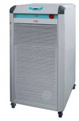
FL7006 Powerful Recirculating Cooler, Julaboo

Figure 4.2: Recirculating cooler FL7006

The figure 4.2 above shows the recirculating cooler that was selected in the beginning considering all the design specifications especially the flow rate of 43L/min. This component for the design was later rejected because it was too expensive and was going out of the budget. The specifications of the chiller is stated below:

Working temperature range from -20 to +40 °C Temperature stability of ±0.5 °C

(41)

39 4.2. Component Selection

Medium: Water Glycol

Pump capacity flow rate of 60 L/min Pump capacity flow pressure of 0.5 to 6 bar Filling volume 39 to 47 L

Dimensions (W × L × H): 78 x 85 x 148 cm

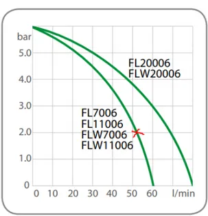
The specifications shown above was clearly within the design that we needed. The figure 4.3 below shows the pump capacity or the flow rate of the pump at different pump pressures. It is clearly understood from the plot that the pump capacity is maximum at the lower pressure ranges. This is also kept in mind during the design.

(42)

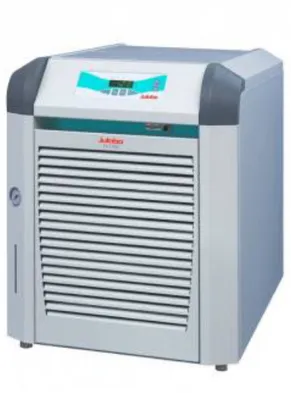
FL1203 Recirculating Cooler, Julaboo

Figure 4.4: Recirculating cooler FL1203

The figure 4.4 above shows the recirculating cooler that was selected in the second stage since the first one was way too much out of the budget considering all the design specifications especially the flow rate of 43L/min. This component for the design was also later rejected even though it was a bit more cheaper but still keeping the overall budget to be big. The specifications of the chiller is stated below:

Working temperature range from -20 to +40°C Temperature stability of ±0.5 °C

Cooling capacity 5kW Medium: Water Glycol

Pump capacity flow rate of 40 L/min Pump capacity flow pressure of 0.5 to 3 bar Filling volume 12 to 17 L

Dimensions (W × L × H): 50 x 76 x 64 cm

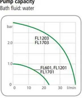
The specifications were almost clearly close to the required ones. The figure 4.5 below shows the pump capacity or the flow rate of the pump at different pump pressures

(43)

similar to the one shown before. The plot shows the pump giving a flow rate of 40 L/min at a pump pressure of 3 bar.

(44)

SMC Thermo Chiller HRS 050-AF-20

From the previous sections, we have got the specifications to be considered to select the pump, reservoir and the cooling unit. A chiller was then selected from SMC which has a reservoir and an in built pump as well. The main specifications of the pump corresponding to the design specifications are as shown below:

a) Tank capacity of 5 litres.

b) Pump capacity of 23 L/min at 2.4 bar.

c) Operating temperature is from 5 to 40 degree Celsius. d) Pressure range from 3 bar to 5 bar

e) The fluid is air cooled with fan inside the chiller.

(45)

Figure 4.7: Working of Thermo Chiller HRS 050-AF-20

The above figure 4.7 shows the working of the chiller HRS 050-AF-20. The chiller consists of a tank with a capacity of 5 litres. The chiller consists of an inlet and an outlet, both with a 1/2 inch port size. The outlet pipe from the tank directly goes to the bottom right side of the chiller which will be connected to the inlet side of the heat sink. A pump is connected to this outlet side which ensures proper pumping of the fluid across the whole experimental setup. The pump has a pump pressure of 5 bar which meets the design specification (3 bar) and also a pump capacity of 23 L/min. A temperature sensor is also available at the outlet which helps to measure the temperature of the fluid leaving the chiller. This can be helpful when the measurements have to be compared with the readings from the senors on the inlet side of the heat sink.

The inlet piping stays on the left top side of the chiller which takes in the fluid from the outlet side of the heat sink. Similar to the outlet side, the inlet side of the chiller provides a temperature sensor which can be used to measure the temperature of the fluid entering the chiller from the heat sink. This can be also used in comparing with the temperature measurements that was taken on the outlet side of the heat sink on the temperature sensors.

(46)

The figure explains the method of cooling where the cooling takes place in an evaporator where the refrigerant gas is used for cooling the fluid that enters the chiller from the heat sink. The mode of cooling is air cooling where a fan is used in a refrigeration unit. This cooling unit also consists of a compressor , a filter and two expansion valves. There are two pressure sensors in the circuit to control low pressure refrigerant gases. A temperature sensor is provided here which keeps the fluid at the temperature that is set to.

The chiller also has a drain port at the bottom right side which helps in draining the fluid used in the chiller at any stage of the testing and can be filled again through the tank in the top. The tank also has a level switch which notifies you on the amount of liquid it can take. All these measurements can be read on the digital screen on the chiller. There are buttons along the screen itself which helps to move through the different values and also to set the temperature of the fluid in the chiller.

The specification table of the chiller is attached along the appendix for better un-derstanding. The chiller can also take mixture of water glycol mixture which is also favourable for the testing. This chiller was selected after proper study and also was within the budget specified.

4.2.2 By-Pass Piping

The by-pass piping set is not a mandatory requirement instead a precautionary control set which can be used to eliminate any pressure buildup at the flow meter at very low flow rates. The calculations were done on the amount of pressure which can be build in case of static flow at the flow meter inlet and the pressure buildup was very minute in the decimal places.

The piping set is very easy to install on the chiller and can be used in case of emergency situations. The pipe takes the extra flow through it back to the tank in the chiller itself avoiding the build up at the flow meter.

The by pass piping is highly recommended in cases where the flow needs to be very low. This is because the chiller provides a continuous supply of fluid at 23 L/min and the flow is controlled at the flow meter to a lower value when needed. This can in turn reduce the chances of efficient cooling and also unwanted pressure developments. For instances like these, the by pass can be used where the extra flow is taken back into the chiller tank itself.

The figure 4.8 below shows the specific model of pass piping set which can be used for the chiller which was selected.

(47)

Figure 4.8: By-Pass Piping set

4.2.3 Flow Meter with Integrated Flow Controller

A flow meter is as important as the chiller to measure the flow at which the system is operating at. A flow controller is also of much importance in this test rig since the chiller will be supplying the flow at a constant flow rate of 23 L/min. The flow rate has to be controlled and should be able to be reduced to different lower values. For this, a flow meter with an integrated option to control the flow is selected from SMC itself. The flow meter can be operated on low values from 5 to high as 40 L/min. It has a display screen that can be used to read the flow rates and adjust the values for the required flow. The flow meter also can take both water and water-glycol mixture.

(48)

The specific flow meter for the test rig was selected from a variety chart depending on the flow rate range, flow controlling option and the fluid that can be used. A port size of 3/4 inch was selected for both the inlet and outlet of the flow meter. The flow meter also has the option with an M8 connection cable that can be attached to a data acquisition system to read the flow. The specifications of the flow meter is shown below. 2 -line display in three colour for easy readout.

Built-in temperature sensor. Very short stabilising section. Compact, space saving design. Flow rate : 5 to 40 L/min.

Medium temperature: 0 to 90 °C.

45° steps rotating display for flexible installation position. No calibration required.

IP65 protection.

(49)

4.2.4 Flow meter MID DN25

In the previous section, the flow meter and controller selected for the test rig was explained. This section describes on the flow meter which was studied in the first phase of the component selection when the flow rate was taken to be 43L/min. This made it clear that the flow meter must be able to take flows which are at least 43L/min. The flow meter can also be used to control the flow to any values from 1 to 80 L/min. This was actually helpful in the case that the flow from the chiller is constant throughout. The figure and specification of the explained flow meter is provided below below. Measurement technology: magnetic-inductive.

Suitable Fluids: Water-Glycol.

Working temperature range: -40°C to +130°C. Flow rate: 1 to 80 L/min.

Fluid connectors: M30x1.5 male. Tubing diameter: DN25.

Output signal: 4 - 20 mA.

Mains power supply: 100-230V/50-60Hz.

Power Supply and 2.5m analog signal cable to connect to PRESTO included. Assembled in frame (Height app. 500mm).

Figure 4.11: Flow meter MID DN25

This flow meter was though later skipped due to the overpricing and was not needed for the new flow rates which were decided on.

(50)

4.2.5 Temperature Sensors

Even though the test rig depends on both types of the sensors for the calculation purposes, the temperature sensors plays the vital role to calculate the thermal efficiency of the heat sinks tested. The temperature sensor used for the test rig should have the lowest reaction time to detect the temperature variation and also should be also highly accurate. A compact temperature sensor was selected for this purpose having an accuracy in the class of Type B 1/10 DIN (0.03+0.005x Tactual).

The sensor has a temperature range up to 200 degree Celsius. The tip of the tempera-ture sensor is made of a smaller diameter than the sensing rod for the high sensitivity and low reaction time. The specifications of the temperature sensor is given below. Sensor diameter: Ø8 (D2) with small sensor tip (D1).

Immersion length: 100mm Extension length: 35mm Process attachment: G1/2” Electrical connection M12 Sensor element: 1xPt100 Number of conductors: 4

Media temperature [max]: Max temperature 200 degree Celsius.

Tolerance in accordance with DIN IEC 751: Type B 1/10 DIN (i.e.±(0,03+0,005xTactual)°C) The temperature sensors were selected with least tolerance variation and of the highest accuracy class. The tolerance range is shown above in the specifications.

(51)

4.2.6 Pressure Sensors

The pressure difference between the heat sink is needed for the proper design and the study of the heat sink. The maximum pressure difference between the heat sink was considered to be 2 bar for the design of the experimental setup. The chiller which was selected has a pump pressure up to 5 bar which can handle any pressure variations in the system. Even though the difference in pressure between the heat sinks was assumed to be 2 bar, for the selection of the pressure sensors, the values were taken from a previous fluid simulation done on the same heat sinks and the maximum pressure difference was found to be as small as 0.25 bar. This is actually important because the pressure range of the sensor plays an important role in the sensitivity of the measurement. So the sensor to be selected should be close to the high value taken from the simulation or a bit above. The specifications of the pressure sensor is shown below.

Ceramic pressure sensor: Standard version:

ECT1.6A 8472.73.5717.05.19.58.61.T2

Pressure range (measurement range): 0. . . 1,6 bar [over pressure safety 3,2 bar]

Accuracy: +/- 0,5 percent of Full scale @ 25 Celsius [ 1,6 bar * 0,005 = +/-0,008 bar] Process connection: G1/4” male

Electrical connection: EN 175301-803-A including DIN43650-A connector Output signal: 4-20mA (power supply 24 VDC)

External O-ring for process connection: FKM material Media temperature:-25°C - +125°C

(52)

4.2.7 Piping, Connectors and Insulation

The main concern regarding the piping are the piping size or the cross sectional area and also the piping length that can be used for the whole test rig. The cross sectional area of the pipe is found with the given design specification and the velocity of 2 m/s. The length of the whole piping should stay within a limit so that the chiller tank capacity is not completely used.

q = AV, (4.2)

where q is the volume flow rate in m3_/s, A is the area of cross section in m2 and V is

the velocity of the flow which is 2 m/s.

q = m/ρ; (4.3)

where m is the mass flow rate which is 23L/min and ρ is the density of the fluid which is considered as 1000 kg/m3 _{for water.}

From these, the diameter of the pipe is calculated to be 0.0156 m or around 15 mm. The length of the whole piping in the experiment rig is calculated from the total volume in the setup,

V = Πr2l (4.4) where, r was found to be 0.015m above and the volume of the tank of the chiller is 5l. From these, the length was found to be around 28 m.

The piping were then selected for calculated design with diameter of 15mm. Other connectors and elbows were also used to complete the building of the test rig.

The sensor holders were also selected with the dimension of the pipe and the sensor connections. 3/4 inch connectors and 1/2 inch connectors were used for the connection at both the inlet and outlet. A figure of the sensor holder is shown below.

(53)

Insulation were also selected to cover around the pipes for better temperature stability and working. The insulation were not installed during the building phase and will only be installed after the first successful running of the test rig without any leakage. The figure below shows the pipe insulation which were used for the test rig.

(54)

4.3 Working

This section describes the working of the test rig in a conceptualized manner with the components selected for the test rig. The chiller selected, pumps the fluid at constant flow rate of 23 L/min and this flow will be later varied to different values from 5 to 23 L/min using the control valve in the flow meter. The chiller also provides the option to control the temperature and the pressure of the fluid leaving the unit. The flow meter will be also used to record mass flow rates. This is either done on the digital screen on the flow meter itself or using data acquisition which is connected through an M8 cable which is also a part of the flow meter. The controlled flow from the flow meter is then led to the inlet sensors at the heat sink where the inlet pressure and temperature of the flow is measured. Temperatures are also measured from the heat sink surface using thermocouples which will be glued to the heat sink. This measurements are later used for the thermal resistance calculations of the heat sink. After the flow leaves the heat sink, the outlet temperature and pressure readings are again measured using the outlet sensors. These temperature measurements are also later used for the final resistance calculation which is explained in equation 4.1. The flow then enters back in the chiller where the temperature of the fluid is controlled to a value which is defined on the chiller.

(55)

Chapter 5 Results

The components were selected and a budget was passed in the company to purchase the components. The final components decided to be purchased is given below.

Chiller ( reservoir + pump + cooler) SMC Thermo Chiller HRS 050-AF-20

Flow meter and controller SMC Digital Flow Switch PF3W740S-F06-BN-M Temperature Sensor Regal RT-B-BP1 Compact temperature sensor Pressure Sensor Regal Ceramic Pressure Sensor

Pipes Copper pipe of internal diameter 15mm

5.1 Preliminary and Final Design

After all the calculations and selection of the components for the test rig, the 3D models were used to design it on Solidedge.The preliminary design (5.1 and 5.2) is shown below. Each component models will be shown in the appendix at the end of the report.

(56)

Chapter 5. Results 54

Figure 5.1: Preliminary Design in top view

The main components on the rig such as the chiller, flow meter and controller, sensor holders for the temperature and pressure sensors are shown in the top view of the design above. The flexible piping next to the left sensor holder gives you the freedom to adjust the length of the pipe so that heat sinks with different dimensions can be installed for testing. A predefined space of 100 mm was left between the sensor holders.

(57)

55 5.1. Preliminary and Final Design

Figure 5.2: Preliminary Design in isometric view

In the beginning stages of building the test rig, the design was slightly modified since the flexible pipes were not suiting their purpose because of their short lengths. Hence,the sensor holder on the right side was directly connected to the flow meter and the left side length was doubled for a longer length and thus a better flexibility helping the purpose.

The figures below shows the final design in the top view and the isometric view. Each component drawings will be shown in the appendix.

(58)

Figure 5.3: Final Design in top view

(59)

57 5.1. Preliminary and Final Design

The figure below shows the real time experimental setup that was build in the flow lab in ABB power grids. The figure shows the chiller on the left as was shown in the Computer Aided Design (CAD) and also the flow meter on the right side on the table. The piping’s and the plumbing work can also be seen in the figure shown below.

Figure 5.5: Experimental Setup Front View

(60)

The sensors, both the temperature and pressure are not installed on the experimental setup. This was due to the lag in delivering the components. These are to be installed before the testing for the temperature and pressure measurements at the outlet and inlet of the heat sinks.

After the measurements are taken from the sensors and from heat sinks, these values are used for the calculation of the thermal resistance of the heat sink, which was discussed in the temperature sensor section, using the equation,

Rth=

Ploss

, (5.1)

where,

(61)

Chapter 6 Discussions and Conclusion

6.1 Discussion

The final design was furthermore evaluated for all the parameters like the velocity of the flow through pipes, total pressure buildup in the whole system, pressure differences at different components. The designed system is compact and is easy to disassemble. Both the pressure and temperature sensors are calibrated at the factory itself and its ready to install and use. All the components selected satisfies the requirement specification of the test rig from discussions and measurements can be taken accurately with the help of high precision sensors.

The preliminary design showed that the flexible piping on both the sides of the heat sink would gives less flexibility due to the size constraints. This was later modified by installing a flexible pipe on one side (outlet side of the heat sink), which provided much more flexibility.

The pump in the chiller will be able to handle any sort of pressure difference in the system with its 5 bar pump pressure. Also the fluid flow can be kept at a constant temperature with continuous cooling by the help of the in built fan within the chiller itself, which has a cooling capacity of 4.7kW. The flow meter is used before the sensors to read the flow rates and also used to control the flow using the integrated controller on it varying from 5 to 40 L/min.

The flexible piping on the inlet side of the chiller helps to test heat sinks of different sizes from 100 to 500 mm which makes the test rig flexible for different size heat sinks. Though this flexible pipe can be a bit stiff when big heat sinks are to be tested and can replaced with a shower set pipe which makes it even more flexible and easy to install the heat sinks on the system.

(62)

Chapter 6. Discussions and Conclusion 60

By pass piping set helps the system for proper cooling and also in case of excess flow when the flow from the chiller is reduced to a lower value using the flow meter. This makes sure the system works smooth without any question of pressure buildup at the flow meter. Also the cooling works at the defined temperature in the chiller.

6.2 Conclusion

The Experimental setup was built successfully with the final design and selected compo-nents. All the components in the experimental setup satisfies the design requirements. The experimental setup can be used to test heat sinks of multiple sizes varying from 100mm to 500mm. The whole test rig was built within the budget that was decided. The components are easy to disassemble. The test rig provides a cooling power of 4.7 kW, promising constant temperature in the system. The pump pressure of 5 bars and the by-pass piping on the chiller eliminates any sort of pressure build up in the test rig. The sensors, both the temperature and the pressure sensors, provide high accuracy measurements than the previous temporary rig. These sensors shows the least variation from the actual value because of the precise tolerance class selected. The experimental setup is aesthetically compact, modular and have a smaller footprint than the tem-porary test rig. Figure 6.1 shows the preferred architecture for the experimental test rig and also the main components that are used in the setup. The main components being the chiller, flow meter and controller, sensor holders to install the temperature and pressure sensors and flexible piping to adjust the size.

(63)

Chapter 7 Recommendations and Future Work

There are some suggestions which can be done on the test rig as a future work and also some installations which are mandatory.

a) The sensors, both the temperature and pressure were not installed due to late delivery. This need to be installed before the testing.

b) The flexible pipe can be replaced with a shower pipe set as explained in the section 6.2 for better flexibility.

c) The thermal insulation is to be installed after the first testing making sure there is no leakage in the system.

d) Testing of different heat sinks on the test rig and validating with the results from the simulations.

(64)

Bibliography

[1] Lokman Hosain. (2019) Hydrodynamic and Thermal Performance Analysis of HVDC G5.1 Full Bridge Middle Heat Sink with Single Inlet-Outlet

[2] Yuhe Jiao. (2019). CFD calculation on performance of HVDC light G4 G5 IGBT heat sink.

[3] Lokman Hosain. (2018). CFD Simulation of Full Bridge Middle Heat Sink [4] Lokman Hosain. (2018). Hydrodynamic and Thermal Performance Analysis of

Full Bridge Middle Heat Sink v2

[5] Azar A. (2009). "Heat sink testing methods and common oversights" [6] Erik van Kemenade. Eindhoven University of Technology ,Department of

mechanical engineering,September 1999 Heat Exchanger Test Rig [7] Orlando Girlanda. (2019). AM of heat sinks for HVDC application

[8] Matthew Wong, Leuan Owen, Chris J. (2009). Pressure Loss and Heat Transfer Through Heat Sinks Produced by Selective Laser Melting

[9] Qi Li, Ludger Fischer, Geng Qiao, Ernesto Mura, Chuan Li, Yulong Ding (2020). High performance cooling of a HVDC converter using a fatty acid ester based phase change dispersion in a heat sink with double layer oblique crossed ribs

[10] Thermal Chamber Heatsink Testing Methods.

https://www.tweaktown.com/articles/1200/thermal chamber heatsink testing methods/index.html

[11] Yunus Cengel. Heat and Mass Transfer

[12] James Welty. Fundamentals of Momentum, Heat and Mass Transfer, 6th Edition International

(65)

63 Bibliography

[13] Samuel D.Marshall, Lakshmi Balasubramaniam, Rerngchai Arayanarakool, BingLi, Poh SengLee, Peter C.Y.Chen.(2017) Methods and techniques of improving experimental testing for microfluidic heat sinks

[14] Kenan Yakut, Nihal Alemdaroglu ,Isak Kotcioglu, Cafer Celik (2006)

Experimental investigation of thermal resistance of a heat sink with hexagonal fins

[15] Mills, A.F., 1999, Heat transfer, Second edition, Prentice Hall. Potter, C. M. Wiggert, D. C. (2002). Mechanics of fluid

[16] White, F. M. (1999). Fluid mechanics

[17] Kim, Seo Young; Koo, Jae-Mo; Kuznetsov, Andrey V. (2001). "Effect of anisotropy in permeability and effective thermal conductivity on thermal performance of an aluminum foam heat sink"

[18] https://www.princeton.edu/asmits/Bicycleweb/Bernoulli.html [19] Chiller specifications and by pass set

https://www.smc.eu/smc/Net/EMC_DDBB/ce_documentation /data/attachments/IMM_HRS050-060_TFR03EN.pdf

(66)