Joint econometric models of freight transport chain and shipment
size choice
Megersa Abate
Swedish National Road and Transport Research Institute (VTI) Inge Vierth
Swedish National Road and Transport Research Institute (VTI) Gerard de Jong
Significance, ITS University of Leeds and Center for Transport Studies, VTI/KTH
CTS Working Paper 2014:9
Abstract
In freight transportation, decisions regarding the choice of transport mode (or chains of modes) and shipment size are closely linked. Building on this basic insight, in this paper we estimate and review various joint econometric models using the Swedish National Commodity Flow surveys. Robust parameter estimates from this exercise will be used to update the current deterministic Swedish national freight model system (the SAMGODS model) to a stochastic one.
Keywords: Discrete–continuous models, Mode choice, shipment size choice, Freight
Modeling
JEL Codes: R0, L91
Centre for Transport Studies SE-100 44 Stockholm
Sweden
1
Joint econometric models of freight transport chain and shipment size
choice
1Megersa Abate* Inge Vierth*
*Swedish National Road and Transport Research Institute (VTI)
Gerard de Jong
Significance, ITS University of Leeds and Center for Transport Studies (VTI/KTH) April 2014
Abstract
In freight transportation, decisions regarding the choice of transport mode (or chains of modes) and shipment size are closely linked. Building on this basic insight, in this paper we estimate and review various joint econometric models using the Swedish National Commodity Flow surveys. Robust parameter estimates from this exercise will be used to update the current deterministic Swedish national freight model system (the SAMGODS model) to a stochastic one.
I. Introduction
The main feature of the current Swedish national freight model system (SAMGODS model) is incorporation of a logistic component in the traditional freight demand-modelling framework. Logistical decisions of firms are incorporated in the modelling process based on shipment size optimization theory. According to this theory, firms are assumed to minimize total annual logistics costs by trading-off inventory holding costs, order costs and transport costs. The logistics module of the SAMGODS model estimates frequency/shipment size choice and transport chain choice (i.e. transport mode choices and use of trans-shipment) based on a deterministic cost minimization model where firms are assumed to minimize annual total logistics costs.
Judged by international standards in freight transport modelling, the SAMGODS model is relatively modern. Its logistic module, however, lacks two main elements. First, it does not
1 This report is funded by Trafikverket through the “Stokastisk logistikmodul” project. This funding is both
acknowledged and gratefully appreciated. Trafikanalys kindly provided the Swedish commodity flow survey data. We would like to thank Christian Overgård, Henrik Edwards and Jonas Westin for their constructive comments. Thanks also toseminar participants at the Center for Transport Studies (CTS) and Trafikverket in Stockholm for helpful suggestions and comments. The usual disclaimer applies.
2
account for the main determinants of shipment size and transport chain choices other than cost, i.e. decisions are mainly based on cost considerations (and to some extent on factors such as access to road and rail and value densities).2 Second, the model is deterministic and lacks a stochastic component. In order to improve the predictions of the model and allow richer policy analyses, logistical decisions should be modeled taking into account these two elements (Section II describes how we intend to carry this out). A full random utility logistic model which accounts for this was planned (SIKA, 2004) but has not yet been estimated on disaggregated data (de Jong and Ben-Akiva, 2007).
This project is a first step towards estimating a full random utility logistic model. Its main objective is to estimate robust econometric models that describe the determinants of transport mode chains and shipment size choices. We use the 2004/2005 Swedish Commodity Flow Survey (CFS) to estimate the choice models.3 The main econometric work in this project involves modelling the interdependence between shipment size and transport chain choices using a joint (e.g. discrete-continuous or discrete-discrete) econometric model. Parameter estimates from this model will later be used for estimation of a full random utility logistic model. They could also be used to estimate transport time and cost elasticities to analyze policy outcomes.
The remaining part of this paper is organized as follows. Section II presents a brief overview of the logistic model component of the current SAMGODS model and outlines of how to implement the stochastic logistic model. Section III presents joint econometric models for the estimation of transport chain and shipment size choices. Section IV describes the data and Section V presents main results. Finally, Section VI presents our main conclusions and suggestions for future work.
2 Various haul, carrier, shipper and commodity characteristics have been shown to be important factors in
determining these decisions (for details, see Abate and de Jong, 2013; Johnson and de Jong, 2011; Holguin-Veras 2002; Abdelwahab and Sargious, 1992; Inaba and Wallace, 1989; McFadden et al. 1986)
3 The initial plan was to use the 2009 CFS. However, we had to use the earlier CFS because we could only
3
II. SAMGODS review
When the logistics model within the aggregate-disaggregate-aggregate (ADA) framework for Sweden (and Norway) was first conceived, the idea was that the logistics model would be estimated on data at individual shipment level from the Swedish Commodity Flow Survey (CFS) (see de Jong and Ben-Akiva, 2007, section 7).
Since the deterministic logistics module as such is complex and the estimation of disaggregate models would take a significant amount of time, a ‘preliminary’ or ‘prototype’ version of the logistics model was developed (see de Jong and Ben-Akiva, 2007, section 8) in 2005/2006. This version did not require disaggregate estimation. Instead it relied on a cost minimisation per firm-to-firm (f2f) flow, where for each f2f flow only one alternative (namely the one with the lowest total logistics cost) is chosen. This method is therefore a deterministic cost minimisation model, which is conceptually equivalent to the all-or-nothing assignment method often used for allocating traffic flows to a network. Because it uses different transport solutions for different firm sizes and shipment sizes, the all-or-nothing character of the deterministic model is reduced.
After the prototype had been developed, it has been improved in a number of rounds and also calibrated to aggregate data for a base year. Although Sweden is one of the few countries in the world in which disaggregate data on freight transport is available (in the form of the CFS), work on estimating disaggregate models was not commissioned until 2013, when the project started work on a stochastic logistics module, reported in this report, and the logistics model within SAMGODS remained a deterministic model.4 The logistics models within the ADA framework for Norway and Flanders are also deterministic models (Ben-Akiva and de Jong, 2013, section 4.6). The Danish national freight model that is being developed at the moment and also follows the ADA setup, contains a module for the choice of mode to cross the Fehmarn Belt screenline that uses a random utility model estimated on disaggregate data (including stated preference SP surveys in the Fehmarn Belt corridor). Other transport chains, however, for example in Denmark, are handled by a deterministic logistics model (Ben-Akiva and de Jong, 2013, section 4.6).
4 Some estimation work involving models for shipment size and mode or transport chain on Swedish CFS data
took place in the meantime at the University of Leeds (e.g. Johnson and de Jong, 2011) and as part of an internship at Significance of a student from Delft University of Technology (Windisch et al., 2010), but also at Swedish universities (Habibi, 2010; Liu, 2012).
4
There are, however, several arguments for going from the current deterministic to a random utility logistics model:
1) A deterministic model has a weak empirical foundation: the way transport agents behave in the model is not based on observed data but on the assumption that they will choose the shipment size and transport chain that has minimum costs (and on data relating to transport networks, possible transhipment locations and expert knowledge of cost functions). Instead of observed behaviour, such a model represents normative behaviour: what would be the outcome if all freight transport agents behaved entirely according to standard economic theory (see also Tavasszy and de Jong, 2014, chapters 6 and 10)? The CFS can provide the main empirical data that is needed here (revealed preference data) for a basis in real life. So far, calibration of the logistics model has only been done at the level of very aggregate OD-level data.
2) This also implies that explanatory factors that are not part of the logistics costs are not included in the model. But the choice of transport chain also depends on factors such as reliability and flexibility of modes. Here the CFS only provides limited information. But at least it contains observed choice information that is the result of all relevant factors together, which makes it possible to estimate constants per transport chain alternative that give the average influence of factors such as reliability. To estimate separate coefficients for the effect of such factors one would need to collect additional data, presumably stated preference data, and estimate a joint model on this data and the CFS (or transfer outcomes from stated preference models from other countries to Sweden, as in the planned transferability project on reliability in freight transport that aims to make use of results of the Norwegian and Dutch SP studies on the value of reliability (Krüger, N; Vierth, I; de Jong, G; Halse A; Killi, M, 2013). However, the task of including these other factors refers to further improvements of the SAMGODS, which will presumably take place after having moved from a deterministic to a (partly) probabilistic model. It is not necessary for a random utility model to include SP evidence; the data in the CFS is good enough for going from a deterministic cost minimisation logistics model to a random utility logistics model (for many of the commodity groups). Every commodity type where we can base the choice mechanism on observed data – for instance, from the CFS – constitutes an improvement relative to the deterministic model. But we can improve the new random utility logistics model in a later phase with the results of (foreign or domestic) SP surveys. Another benefit of
5
these SP surveys is that that they can lead to better-founded values of reliability for use in cost-benefit analysis.
3) A well-known disadvantage of deterministic models (which can also be a feature of all-or-nothing traffic assignments) is that the impact of changes in scenario variables (e.g. oil prices) or policy variables (e.g. a new road, railway or terminal) can lead to an implausibly large response, so-called ‘overshooting’ or ‘flip-flop’ behaviour. This happens when the relevant part of the logistics costs function is rather flat and a small change in logistics costs can lead to a shift to a completely different optimum shipment size and transport chain. This phenomenon does not always arise, and it is corrected to some degree by using a large number of different f2f flows in the model, which do not have to move in the same way. And if the optimal alternative has much lower logistics costs than the second-best alternative, the model behaviour could be very stable. But the possibility of flip-flop behaviour is present and it has been noted that the SAMGODS model in some cases behaves too shakily to make a proper comparison of a reference case and a project case for cost-benefit analysis. However, the Swedish shipper market is quite concentrated, which implies that large shippers or the logistic decisions of single large shippers can influence the overall modal split.5
Issues 1 and 3 above can be solved by estimating disaggregate random utility models on the CFS data: the observed shipment level data will then form the empirical basis for the behavioural coefficients of the model. By their nature these are probabilistic models because they include a stochastic component to account for the influence of omitted factors. A deterministic model effectively assumes that the stochastic component can be ignored – in other words, that the researcher has full knowledge of all the drivers of behaviour and that there is no randomness in actual behaviour. As a result of adding the stochastic component in the random utility model, the response functions (now expressed in the form of probabilities) become smooth instead of lumped at 0 and 1 as in a deterministic model. The project on the stochastic logistics module that is reported in this report is carrying out exactly this disaggregate estimation. On issue 2: the CFS does not contain information that includes the softer factors may also influence the choice of shipment size and transport chain, but since it contains the information on choices really made, one can estimate constants per transport
6
chain alternative that give the average influence of these factors (besides the influence of the stochastic component).
The disaggregate models that are tested in the stochastic logistics module project are estimated for various commodity categories separately, but not necessarily for all commodity groups that are in the current SAMGODS (the estimation project also does not include imports flows into Sweden, which are in the current SAMGODS).
This project is only an estimation project. To establish a version of SAMGODS that is based on random utility modelling, the following further steps are required:
a. Extend coverage to all commodities (and directions) and move from the extended NSTR classification to the NST 2007 classification for commodities
If the estimated models do not cover all commodities (and directions, such as missing imports) that should be covered in SAMGODS, one must determine which behavioural rules should be used for any missing commodities (e.g. by further estimation, by relating to a similar commodity for which a model was estimated or by keeping a deterministic model for these commodities). Determining these rules should not require much work (a few person-days), unless further estimation is involved, which could take several additional months if all commodity groups are covered and can be taken from the CFS. A new model version of SAMGODS will use a random utility formulation for some of the commodities, but deterministic cost minimisation for other commodities is feasible since they are independent in the model.
The next version of the SAMGODS model will be based on NST 2007 as commodity classification. This is very different from the NST/R classification that the CFS 2004/2005 uses (CFS 2009 uses NST 2007). To maximize the possible use of models that are estimated on the CFS 2004/2005, it is best to concentrate on commodities that can be translated one-to-one from the CFS 2004/2005 to the new model that will be based on NST 2007 (or where the conversion is straightforward). Later we may have to estimate further models on CFS 2009 and future CFSs.
The move from the extended NSTR commodity classification to the NST 2007 classification has to be synchronised with the ongoing update of the zone-to-zone base matrices (production-warehouse-consumption matrices, PWC matrices). As for the actual matrices
7
(CFS 2001 and CFS 2004/2005), the commodity flow survey (next CFS) is one of the main data sources for estimating the PWC matrices.
b. Determine the annual firm-to-firm flows
For the probabilistic model, the routines to generate firm-to-firm flows (from the zone-to-zone flows) can remain as they are. The new models will be applied at the level of these firm-to-firm flows, so as input for the logistics choices we will know the annual firm-to-firm-to-firm-to-firm demand Q, as well as transport time and cost for all available transport chain and shipment size alternatives.
c. Determine the input for applying the utility functions
The utility functions that are estimated in this project are similar to the current total logistics costs formulations. An important difference is that some of the cost components and some of the parameters (e.g. order costs, implied discount rate on the inventories in transit and in the warehouse or a value of time; see de Jong and Ben-Akiva, 2007, section 4) have now been estimated instead of given an assumed value by logistics cost experts.6 But for the application of the estimated utility functions we will still need transport distance and time for the available shipments size and transport chains combinations. In the current logistics model, this is done by the BuildChain routine within SAMGODS. The new BuildChain program can remain similar to the current version, but adapted to reflect the more limited number of available chain types. In principle this work has already been carried out in order to provide input data for the estimation in this estimation project. However, this refers to 2004/2005. If one wants to apply the model for later years (including future years), new networks and new assumptions on the transhipment locations need to be made, new network skims need to be made to determine the optimal routes per transport chain and new assumptions need to be made on the magnitude of various components of the logistics cost functions.
d. Implementation of the utility functions and their coefficients to determine shipment size and transport chain choice probabilities
In the current logistics model, the routine where the choice of shipment size and transport chain is determined is called ChainChoi. This is the part of the model that needs to be
6 In the current implementation of the logistics model in SAMGODS, the cost of deterioration and damage
during transit and stockout costs are not included. The CFS does not contain information to explicitly include these components in the random utility functions, either.
8
considerably re-programmed when moving to a random utility model. In a random utility setting, ChainChoi needs to determine the expected shipment size and probabilities for each of the transport chain alternatives for each annual f2f flow in the model and then sum shipments and probabilities over f2f flows.
In equation form what the logistics model does is to determine the sequence (for each flow of commodity k from firm m to firm n):
q l,
q,
h1 1, t
, h2, t2
, ,
h ti, i
, ...,
hIl
, (1)
Where q is the shipment size (the same over the whole transport chain, though it can be consolidated with other shipments), l is the transport chain, h is a mode used on a leg of the chain and t is the next transhipment location. The index I, i=1, … Il denotes a leg of a
transport chain (chain l has Il legs).
Since we do not observe the transhipment locations ti in the CFS, we cannot include this
choice in estimation. Therefore we keep the split between the determination of the optimal transhipment points and the choice of transport chain separate as in the current model. The determination of the optimal transhipment locations for each available chain type from the set of available locations will be done in BuildChain, as in the present model. The random utility model in the new ChainChoi program will refer to the problem:
q l, , {q (h1 1| ) (t , h2 |t2), , (hi | )ti , ...,
hIl }, (2) The deterministic version of ChainChoi solved this problem by finding a single (least cost) transport chain and shipment size alternative for each annual flow of commodity k from m to n. The probabilistic model then replaces this for specific commodities. We will now calculate for the f2f flow a number of probabilities, one for every available alternative. For instance, for an alternative j (say an alternative with shipment size (class) q0 and direct road transport astransport chain), the probability is:
,
/
,
{ , }
P q l j exp Uj q l exp U q l
, (3)
The numerator is the exponentiated utility function of alternative j, whereas the denominator is the sum over all available alternatives {q,l} of their exponentiated utilities.
These probabilities can be summed at the level of the origins and the destinations of the individual legs (e.g. from the sender m to the first transhipment location) over all f2f flows
9
(and weighted by the volume of the annual flows) and by commodity type to get the OD matrices (as in the Swedish national passenger transport model SAMPERS, where application also involves summing probabilities). In calculating the transport costs, consolidation can be handled in the usual way, except that the volume using a certain mode between two transhipment points from a previous iteration will now also be based on a summation of probabilities. What becomes more difficult is to get a vehicle load factor at the level of the f2f flow (since we only have a probability per transport chain), but vehicle load factors per OD and commodity are possible. To take rail capacity restrictions into account, the Linear Programming model can also still be used, though one will need to test how effective increasing the cost for certain rail alternatives will be in the new setup.
In terms of its dimensions, SAMGODS will probably need to be simplified, since the number of different models estimated for different commodity groups will be smaller than the number of commodities in the present SAMGODS (35). The number of transport chain alternatives in the estimated models will also be smaller than in the current SAMGODS (67), as will be the number of vehicle/vessel types (35), mainly because of a lack of more detailed information in the CFS. If the Transport Administration should wish to include more transport chains or vehicle/vessel types than can be managed in model estimation on the CFS, this could be made possible by combining the estimated random utility models with deterministic models for the allocation to finer categories given the outcomes of the former models. It will still be possible to use the 35 commodity-specific values for the cost parameters (inventory costs, order costs ...), but groups of commodities will share the same cost coefficient in the utility functions. So it will still be possible that the model is operated on 35 separate commodities, but not all commodities will have their own set of model coefficients.
e. Testing and validating the implemented model
Finally, a test and validation of the resulting OD flows by mode against observed aggregate data for a (new) base year is recommended, since a model estimated on one data set (CFS flows) will not necessarily match with other data, such as traffic counts.
10
III. Econometric framework
Econometric studies of freight mode/vehicle choice are based on the key insight that mode/vehicle choice entails simultaneous decisions on how much to ship (see, for example, Abate and de Jong, 2013; Johnson and de Jong, 2011; Holguin-Veras, 2002; Abdelwahab and Sargious, 1992; Inaba and Wallace, 1989; McFadden et al., 1986). This simultaneity in decisions requires the use of joint econometric techniques such as discrete-continuous models.7 In addition to recognizing this simultaneous decision process, these studies show that
various haul, carrier, and commodity characteristics affect the decisions regarding the optimal shipment size choice and choice of transport mode.8
McFadden et al. (1985) and Abdelwahab and Sargious (1992) provide the most complete formulation of the firm’s simultaneous choice of mode and shipment size. However, the applicability of their models is rather limited when decision makers have to choose from more than two mode alternatives. Holguin-Veras (2002) and Johnson and de Jong (2011) used an indirect approach to address the simultaneity problem. They model the discrete choice component (vehicle class choice in Holguin-Veras and mode choice in Johnson and de Jong) as the structural equation of interest, replacing actual shipment with prediction from a shipment size auxiliary regression. This approach is an interesting one when the main focus is the vehicle/mode choice because it is possible to apply advanced discrete choice models that overcome the independence of irrelevant alternatives (IIA) problem that most selection models suffer from. But, unlike McFadden et al. (1985), this approach does not allow for testing for simultaneity bias.
Due to the above technical complexities, mode choice in freight transport is usually studied in isolation (or in combination with network assignment, as multi-modal assignment). However, as pointed out by Johnson and de Jong (2011: 1), mode and shipment size are closely linked decisions. Large shipment sizes usually coincide with higher market shares for non-road transport, whereas there is a high correlation between road transport and small shipment sizes. In search of robust parameter estimates, in this project we formulate and review three disaggregate models specified as: an independent mode choice model (which is the most
7An alternative is sometimes discrete-discrete (by classifying shipment sizes to a number of size classes), as in
Johnson and de Jong and (2011) and Windisch et al. (2010), using Swedish CFSs of 2001 and 2004/2005, respectively.
8 While we only consider the weight of shipment size as an endogenous variable, we note that shipment volume
(in m3) is also an important factor, which shippers consider jointly with mode choice decisions. We cannot
11
common formulation), a joint model with discrete mode and discrete shipment size choice, and a joint model with discrete mode and continuous shipment size choice. The models are specified as follows:
1. An independent mode choice model 1 1 11
Ui X (4)
2. A joint model with discrete mode and discrete shipment size choice 2 2 2 2 2 2
Ui X G (5)
3. A joint model with discrete mode and continuous shipment size choice 3 3 3 3 3 3
Ui X G (6.1)
3 32 3 32
SSi G (6.2)
where:
- Ui1 and Ui3 are the utilities derived from mode i in models 1 and 3, respectively
- Ui2 is the utility derived from a discrete combination of mode i and shipment size
- X1 , X2 and X3 are vectors of independent variables explaining mode choice
- G2 and G3 are vectors of independent variables explaining shipment size choice
- 1, 2, 3, 32, 2, 3 are vectors of parameters to be estimated
- SSi3 is shipment sizefor modei
- 1 ,2, 3 and 32 are error terms
Equation 1 is a simple multinomial choice model formulation that only considers mode choice decisions of firms. The probability of choosing a given mode of transport is a negative function of transport cost and transport time, the two most common explanatory variables in X1. Although its formulation allows for application of advanced discrete choice models, a formulation such as equation 4 disregards the influence of shipment size choice decisions. Equation 5 is a more advanced formulation that accounts for shipment sizes. Here U12 is the
utility derived from the choice of a discrete combination of mode and shipment size choice. As well as explanatory variables that affect mode choice (X2), it controls for an additional set
12
Earlier works (de Jong, 2007; Windisch, 2009) on the Swedish CFSs estimated both mode and shipment size as discrete choices, but clearly shipment size is a continuous variable.9
Johnson and de Jong (2011) correctly noted that both assuming independence between mode and shipment size choice and discretising the continuous information on shipment size may be interpreted as forms of specification error. Model 3 overcomes this basic problem by estimating a joint discrete-continuous model of mode-shipment size model. Equation 6.1 is the discrete mode choice model and equation 6.2 is a continuous part for shipment size. Note that the two error terms, 3 and 32, are correlated because of the possibility that the
transport planner makes a choice between transport chains and at the same time decides how much to load on the chosen transport modes. We note that decisions on the optimal shipment size and mode are generated from the same optimization problem, which implies that the error terms are likely to be correlated. Ignoring this correlation would lead to a specification bias. For this reason we need to model mode choice and shipment size choice using a discrete-continuous model. Accordingly, we rely on a basic econometric model developed by Dubin and McFadden (1984) to address this bias in the context of a polychotomous-continuous choice. A multinomial logit model (MNL) of mode choice is estimated in the first step (equation 6.1) followed by estimation of the shipment size equation (6.2) given the mode choice decision (see Abate and de Jong, 2014, for details of how to apply Dubin and McFadden’s model in freight transport demand modelling context).
IV. Data
The main data source for this project is the 2004/2005 Swedish Commodity Flow Survey (CFS). The data has 2,986,259 records. Each record is a shipment to/from a company in Sweden, with information on origin, destination, modes, weight and value of the shipment, sector of the sending firm, commodity type, access to rail tracks and quays, etc.10 From this we selected a file of around 2,897,010 outgoing shipments (domestic transport and export, no import) for which we have complete information on all the endogenous and exogenous variables.
Although the CFS data is extensive, it does not contain information on important variables such as transport costs and transport time. Given the importance of these variables in
9 Windisch’s and de Jong’s models are based on the Swedish 2004/2005 and 2001 CFSs, respectively.
10In the CFS a shipment is defined as a unique delivery of goods with the same commodity code to/from the
13
mode/shipment size choice analysis, the logistic module of the SAMGODS model was used to generate transport cost and time variables for each shipment in the CFS based on a number of the transport mode chain and shipment size combinations (see below for definition of these combinations).11 These variables were generated both for the chosen mode-shipment alternatives in the CFS and for potential non-chosen alternatives tailored to each shipper based on the transport network of the origin and destination of their shipment.
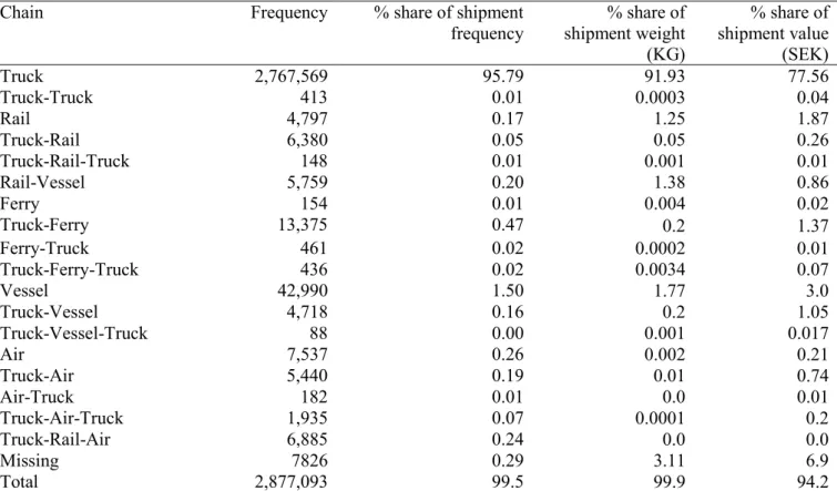
The CFS classifies transport mode chains to chains inside Sweden and chains outside Sweden. Table 1 presents the distribution of transport chains inside Sweden (the number of times each option is chosen). Trucking accounts for the overwhelming majority of the shipments (95.79%), followed by chains which involve waterborne transport modes (a ship vessel and ferry).12 The high share of trucking is also evident in its percentage share in weight and value
of the whole shipments. Table 2 presents similar distributions for international shipments. As seen, vessel transport accounts for the highest share of international shipments in terms of share in total frequency, shipment weight and value.
11 This task was undertaken by Jaap Baak from Significance. The cost functions used for choice set generation
are outlined in de Jong et al. (2010).
12 We defined transport chain alternatives based on their frequency in the CFS. Transportation chains that
occurred with a frequency of 96 or higher were considered as possible choice options.
14
Table 1: Domestic transport chains for outgoing shipments- as stated in the 2004/2005 CFS
Chain Frequency % share of shipment frequency % share of shipment weight (KG) % share of shipment value (SEK) Truck 2,767,569 95.79 91.93 77.56 Truck-Truck 413 0.01 0.0003 0.04 Rail 4,797 0.17 1.25 1.87 Truck-Rail 6,380 0.05 0.05 0.26 Truck-Rail-Truck 148 0.01 0.001 0.01 Rail-Vessel 5,759 0.20 1.38 0.86 Ferry 154 0.01 0.004 0.02 Truck-Ferry 13,375 0.47 0.2 1.37 Ferry-Truck 461 0.02 0.0002 0.01 Truck-Ferry-Truck 436 0.02 0.0034 0.07 Vessel 42,990 1.50 1.77 3.0 Truck-Vessel 4,718 0.16 0.2 1.05 Truck-Vessel-Truck 88 0.00 0.001 0.017 Air 7,537 0.26 0.002 0.21 Truck-Air 5,440 0.19 0.01 0.74 Air-Truck 182 0.01 0.0 0.01 Truck-Air-Truck 1,935 0.07 0.0001 0.2 Truck-Rail-Air 6,885 0.24 0.0 0.0 Missing 7826 0.29 3.11 6.9 Total 2,877,093 99.5 99.9 94.2
Table 2: International transport chains for outgoing shipments- inside and outside Sweden as stated in the 2004/2005 CFS
Chain Frequency % share of shipment frequency % share of shipment weight (KG) % share of shipment value (SEK) Truck 90,851 48.33 3.19 11.81 Truck-Truck 171 0.10 0.005 0.12 Rail 910 0.53 0.93 1.37 Truck-Rail 54 0.03 0.03 0.03 Truck-Rail-Truck 19 0.01 0.01 0.02 Rail-Truck 582 0.34 0.47 0.56 Rail-Vessel 33 0.02 0.05 0.02 Truck-Rail-Ferry 203 0.12 0.06 0.04 Ferry 342 0.20 0.36 0.67 Truck-Ferry 1,659 0.97 0.24 0.71 Ferry-Truck 32,701 19.18 5.15 13.75 Ferry-Rail 118 0.07 0.25 0.55 Ferry-Rail-Truck 116 0.07 0.07 0.12 Truck-Ferry-Truck 1,069 0.63 0.14 0.38 Vessel 25,303 13.46 64.07 46.52 Truck-Vessel 790 0.46 0.15 0.40 Vessel-Truck 13.46 1.94 2.16 3.44 Truck-Vessel-Truck 92 0.05 0.02 0.06 Vessel-Rail 563 0.30 17.99 2.77 Air 6,825 3.92 0.12 1.41 Truck-Air 1,059 0.59 0.003 0.51 Air-Truck 8,620 4.59 0.11 3.82 Truck-Air-Truck 3,078 1.64 0.004 1.34 Total 175,023 97.6 95.6 90.4
15
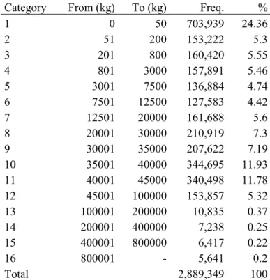
To see the distribution of shipment sizes we classified the continuous weight variable in the CFS into 16 categories, as shown in Table 3. A quarter of the total shipments fall in the first category (0-50 kg). This prevalence of small shipments reflects the dominance of trucking which is usually preferred for its flexibility and reliability. Categories 10 and 11, ranging from 35 to 45 tonnes, account for 23.71 per cent. These are also well within a full truckload range, again showing the dominant role of trucking.
Table 3: Weight categories inside and outside Sweden, as stated in the 2004/2005 CFS Category From (kg) To (kg) Freq. %
1 0 50 703,939 24.36 2 51 200 153,222 5.3 3 201 800 160,420 5.55 4 801 3000 157,891 5.46 5 3001 7500 136,884 4.74 6 7501 12500 127,583 4.42 7 12501 20000 161,688 5.6 8 20001 30000 210,919 7.3 9 30001 35000 207,622 7.19 10 35001 40000 344,695 11.93 11 40001 45000 340,498 11.78 12 45001 100000 153,857 5.32 13 100001 200000 10,835 0.37 14 200001 400000 7,238 0.25 15 400001 800000 6,417 0.22 16 800001 - 5,641 0.2 Total 2,889,349 100
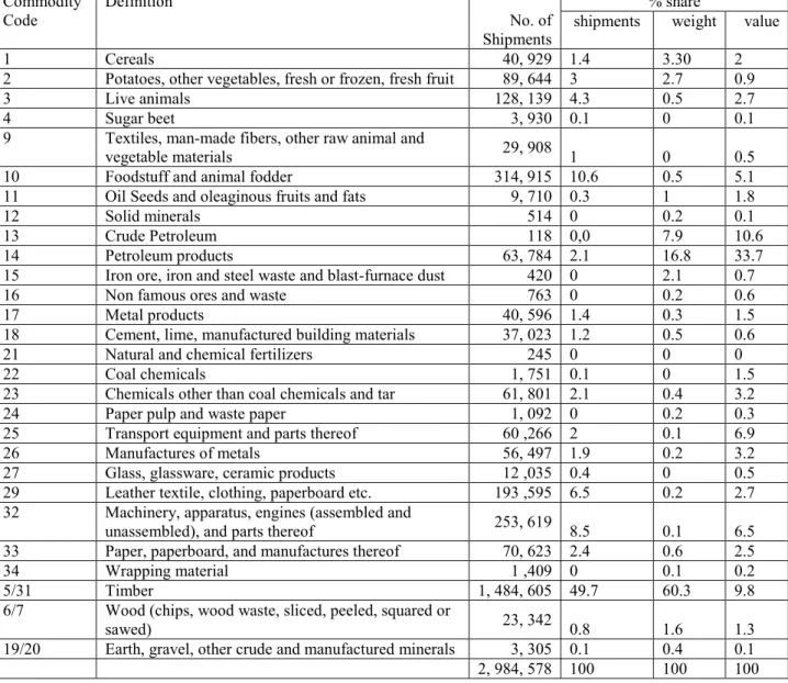
Table 4 presents the commodity groups in the whole (both incoming and outgoing shipments) 2004/2005 CFS. Four commodity groups (Timber, Foodstuff and animal fodder, Machineries, Leather and Textile, Live animals) constitute about 80 per cent of the total shipments. It is important to note here that the 2004/2005 CFS comes from two sources. The first is a sample survey for mining, manufacturing and the wholesale sectors. The second source is a register-based survey for forest and logging products, sugar beet cultivation, and dairy products (this is a reason why timber accounts for half (49.7 per cent) of the whole CFS).13 The table also reports average value and weight per shipment for each commodity group.
13 The register data for timber flows are not door-to-door flows (PWC flows) but do only comprise OD-links for
road. For the time being, Trafikanalys is carrying out a pre-study with the goal of including the whole transport chain for timber (Henrik Pettersson, Trafikanalys, 27 February 2014).
16
Table 4: Share of different commodity groups in the CFS 2004/2005 (both outgoing and incoming shipments)
Commodity
Code Definition No. of
Shipments
% share
shipments weight value
1 Cereals 40, 929 1.4 3.30 2
2 Potatoes, other vegetables, fresh or frozen, fresh fruit 89, 644 3 2.7 0.9
3 Live animals 128, 139 4.3 0.5 2.7
4 Sugar beet 3, 930 0.1 0 0.1
9 Textiles, man-made fibers, other raw animal and
vegetable materials 29, 908 1 0 0.5
10 Foodstuff and animal fodder 314, 915 10.6 0.5 5.1
11 Oil Seeds and oleaginous fruits and fats 9, 710 0.3 1 1.8
12 Solid minerals 514 0 0.2 0.1
13 Crude Petroleum 118 0,0 7.9 10.6
14 Petroleum products 63, 784 2.1 16.8 33.7
15 Iron ore, iron and steel waste and blast-furnace dust 420 0 2.1 0.7
16 Non famous ores and waste 763 0 0.2 0.6
17 Metal products 40, 596 1.4 0.3 1.5
18 Cement, lime, manufactured building materials 37, 023 1.2 0.5 0.6
21 Natural and chemical fertilizers 245 0 0 0
22 Coal chemicals 1, 751 0.1 0 1.5
23 Chemicals other than coal chemicals and tar 61, 801 2.1 0.4 3.2
24 Paper pulp and waste paper 1, 092 0 0.2 0.3
25 Transport equipment and parts thereof 60 ,266 2 0.1 6.9
26 Manufactures of metals 56, 497 1.9 0.2 3.2
27 Glass, glassware, ceramic products 12 ,035 0.4 0 0.5
29 Leather textile, clothing, paperboard etc. 193 ,595 6.5 0.2 2.7 32 Machinery, apparatus, engines (assembled and
unassembled), and parts thereof 253, 619 8.5 0.1 6.5 33 Paper, paperboard, and manufactures thereof 70, 623 2.4 0.6 2.5
34 Wrapping material 1 ,409 0 0.1 0.2
5/31 Timber 1, 484, 605 49.7 60.3 9.8
6/7 Wood (chips, wood waste, sliced, peeled, squared or
sawed) 23, 342 0.8 1.6 1.3
19/20 Earth, gravel, other crude and manufactured minerals 3, 305 0.1 0.4 0.1 2, 984, 578 100 100 100 Since the main objective of this project is finding the best estimation techniques and robust parameter estimates from the joint modelling of transport mode chain and shipment size choice decisions, we focus in this paper on two commodity groups from the CFS, metal products and chemical products, and conduct an in-depth analysis. In Section V, we also review results from previous studies that used the Swedish CFS to get an idea of the robustness of parameter estimates when some of these techniques are applied on all commodity groups in the CFS.
17
At this stage of the project it is more instructive to analyze selected commodities than all commodities identified in the CFS for a number of reasons. First and foremost, as shown in Table 1, trucking is the most dominant transport chain. In fact, for ten commodity groups (namely, groups 1, 2, 3, 4, 10, 12, 13, 14, 21 and 31) the share of trucking is more than 98 per cent. Clearly, there is little to learn about the determinants of mode choice decisions of shippers when there is such overwhelming dominance by one mode of transport. For the remaining 16 commodity groups (including metal products and chemical products, analyzed in depth here) there is relatively less dominance by trucking. In future studies, one has to look at these groups of commodities to get more insights into the mode/shipment size decisions. The second reason for looking at selected commodities is the change of commodity classification from NSTR to NST 2007. The chosen commodity groups should ideally be easily comparable in the two classification systems to ease transferability of parameter estimates between different CFSs. Third, due to problems with the recorded transport chains in the CFS data and transport network, generating transport cost data inputs has proved problematic. In addition to metal products and chemical products, we tried to include other commodity groups from the sub-group of 16 commodities where trucking is less dominant. However, we haven’t managed to replicate the transport chains in the CFS in a reasonable manner in the cost estimation exercise. In future studies, the remaining commodities should be closely investigated. Finally, narrowing the number commodity groups is also necessary to ease the implementation of advanced modelling techniques (applying some discrete choice models on about 2.9 million observations is daunting, if not impossible).
We applied two estimation techniques, namely discrete (equation 5) and discrete-continuous (equations 6.1 and 6.2), using observations form the metal products commodity group. As for chemical products commodity groups, we applied only the discrete-continuous models. For the discrete mode and discrete shipment size model, we classified the continuous weight variable from the CFS into 16 categories (similar to those in Table 3 above). Table 5A shows distribution of transport chains for metal products. Five main transport chains, namely Truck (93.58 per cent), Rail (4.13 per cent), Truck-Rail-Truck (0.10 per cent) Truck-Ferry-Truck (1.77 per cent) and Truck-Ferry-Truck-Vessel-Truck-Ferry-Truck (0.42 per cent), were recorded in the CFS. The most common shipment size category for metal products is category 1 (0–50 kg), similar to the general pattern in the whole CFS data.
18
Table 5A: Domestic transport chains for outgoing shipments - metal products Chain Frequency % share of shipment
frequency % share of shipment weight (KG) % share of shipment value (SEK) Truck 36,822 94.06 22.86 48.4 Rail 1,784 4.56 9.16 23.67 Vessel 127 0.32 63.64 16.41 Truck-Rail 59 0.15 0.91 2.23 Truck-Ferry 182 0.46 0.81 2.41 Truck-Vessel 15 0.04 0.55 0.69 Truck-Air 7 0.02 0.00 0.75 Rail-Truck 5 0.01 0.16 0.36 Rail-Ferry 1 0.00 0.00 0.00 Truck-Ferry-Truck 26 0.07 0.29 0.78 Truck-Vessel-Truck 2 0.01 0.05 0.08 Missing 86 0.21 1.34 3 Total 39,116 100 100 100
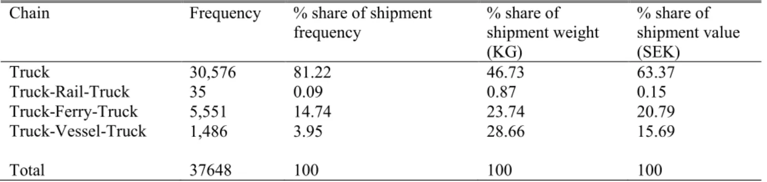
Table 5B: Domestic transport chains for outgoing shipments - chemical products – modeled
Chain Frequency % share of shipment frequency % share of shipment weight (KG) % share of shipment value (SEK) Truck 30,576 81.22 46.73 63.37 Truck-Rail-Truck 35 0.09 0.87 0.15 Truck-Ferry-Truck 5,551 14.74 23.74 20.79 Truck-Vessel-Truck 1,486 3.95 28.66 15.69 Total 37648 100 100 100
Table 5B shows the distribution of transport chains for chemical products. Note that all transport chain alternatives start and end with trucking. Mode choice entries in the CFS where rail, ferry and vessel are stated as the only used mode needed to be updated. This is because in reality, shippers of such products often use trucks in the first and final legs of a transport chain. Furthermore, judged by the location of shippers in the CFS and the transport network available to them, trucking is needed both at the first and the last leg to access other modes of transport. Finally, in order to estimate transport cost and time variables for chosen and non-chosen alternatives, adding trucking at either end was also necessary.14
14 This is a rather pragmatic solution. In future studies the validity of such an assumption should be closely
investigated on a commodity by commodity basis. Future design and collection of the CFS can address some of these problems by asking questions which solicit all the transport modes used for a shipment.
19
Descriptive statistics are given in Table 6 for the whole CFS, metal products and chemical products. As seen for 2 per cent of the total shipments in the CFS, senders had access to rail at origin and 0.4 per cent of them had access to quay at origin. The equivalent figures for metal products (chemical products) are 57 (0.03) per cent and 0.5 (0.03) per cent, respectively. It appears that average shipment values are somewhat comparable, whereas average shipment weights of metal products and chemical products are much less than their whole CFS equivalent. Furthermore, on a per shipment basis, to ship an average metal product (chemical product) shipment, it costs SEK 3,684 (6,783) and takes 3.5 (10.37) hours. The average shipment distances are 256 km and 616 km, respectively.
Table 6: Descriptive statistics
Mean All
Commodities
Metal products1 Chemical Products
Rail access (%) 2 57 0.03
Quay access (%) 0.4 0.5 0.03
Shipment weight (KG) 26,011 6,556 4,023
Shipment value (SEK) 37,122 31,943 42,907
Value density2 (SEK/KG) 1,231 24 288
Transport costs (SEK) 3,684 6,783
Transport time (hours) 3.5 10.37
Transport distance 256 616
No. of observations 2,897,175 34,627 37,648
1 Metal products include pig iron, crude steel, iron alloys, rolled steel, beams, wired rods, steel plates,
strip sheets and non-ferrous metal.
2 Note that the mean of the value density variable is not calculated by dividing the mean values of
shipment value and weight for the whole sample. It is calculated as the mean of the value density for each shipment in the CFS. The two values could be close to each other if both variables are greater than or equal to one. For some observations, however, the weight and value variables are recorded as having values less than one in the CFS, which explains the difference between the two statistics.
Econometric results
This section presents results from the econometric specifications outlined in section III. Since our main objective in this paper is to find robust parameter estimates of transport chain and shipment size choice models, we present results both from previous studies which used the Swedish CFS and from those obtained during the course of this project.
20
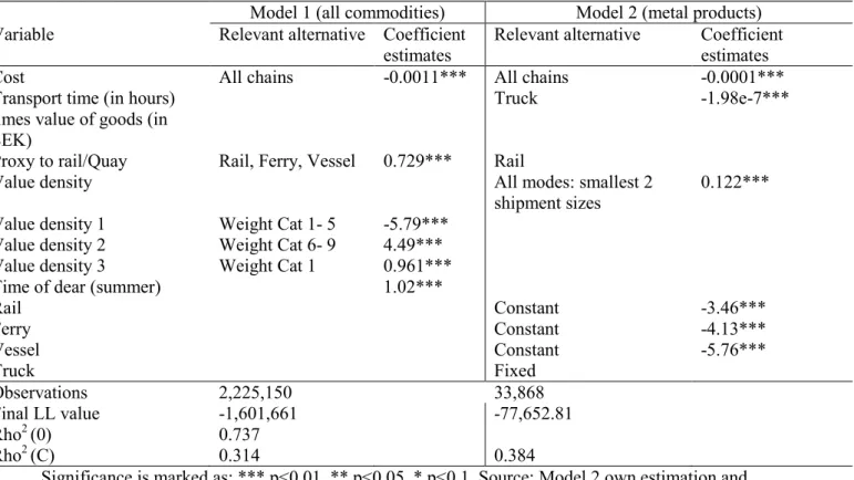
Table 7 presents results from two Multinomial Logit (MNL) models based on the discrete-discrete model (equation 5) using the 2004/2005 CFS.15 Results under model 1 are from Windisch (2009) for all commodity groups but limited to outgoing shipments inside Sweden. Those under model 1 are from the current project and are only for metal products (outgoing shipments inside and outside Sweden). As expected, in both models transport cost has a negative effect on the utility of a choice alternative, implying that higher delivery costs make a choice alternative less attractive. The cost parameter estimate is higher by a factor of 10 under model 1 than under model 2. This is probably due to the higher number of observations used in model 1. However, in both models the effect of cost is rather too low.16
Table 7: Multinomial logit model of discrete shipment size and transport chain choice Model 1 (all commodities) Model 2 (metal products) Variable Relevant alternative Coefficient
estimates
Relevant alternative Coefficient estimates
Cost All chains -0.0011*** All chains -0.0001***
Transport time (in hours) times value of goods (in SEK)
Truck -1.98e-7***
Proxy to rail/Quay Rail, Ferry, Vessel 0.729*** Rail
Value density All modes: smallest 2
shipment sizes
0.122*** Value density 1 Weight Cat 1- 5 -5.79***
Value density 2 Weight Cat 6- 9 4.49*** Value density 3 Weight Cat 1 0.961***
Time of dear (summer) 1.02***
Rail Constant -3.46*** Ferry Constant -4.13*** Vessel Constant -5.76*** Truck Fixed Observations 2,225,150 33,868 Final LL value -1,601,661 -77,652.81 Rho2 (0) 0.737 Rho2 (C) 0.314 0.384
Significance is marked as: *** p<0.01, ** p<0.05, * p<0.1. Source: Model 2 own estimation and Model 1 Windisch (2009)
Under model 2 the variable for inventory costs during truck transport (transport time times value of the shipment) has the right (negative) sign and is highly significant. This variable
15 Note that for consistent estimation of standard discrete choice models (such as MNL) it is not necessary to
re-weight the observations (e.g. using the CFS re-weighting factors). On an exogenously selected sample, as it is the case with the CFS, consistent estimates will be obtained.
16 A more meaningful comparison of results from different discrete choice models is a comparison of elasticities.
21
captures time costs related to the capital cost of the inventory in transit and maybe also to deterioration and safety stock considerations. For truck transport this turns out to be statistically significant, but the point estimates are rather too low. We expect to find a more meaningful effect if the same model is applied on more commodity groups.
For model 1 we see that the dummy variables for rail and quay proximity have significant positive parameters. These dummy variables were only included in the utility functions of choice alternatives where the mode rail and/or vessel were used as first or second mode in the chosen transportation chain. The interpretation of the parameter values is that shippers located in the proximity of rail and/or quay docking facilities are more likely to choose chains that start with a rail or vessel leg (or use these modes on the second leg of the chain).17
In both models we see a significant positive effect for the value density variable. This implies that high value densities correlate with smaller shipment sizes, which might also imply frequent shipments. For model 2 the transportation chain-specific constants all show a negative sign, implying that all transportation chains are less attractive compared to the ‘truck’ chain. This is expected given that the reference chain type, chain type 1 (‘Truck’), is usually chosen for its flexibility and ease of access. While the results reported in Table 7 are plausible, they come from a model in which shipment size is treated as a discrete variable, when shipment size is clearly a continuous variable.18 What follows presents results from theoretically sound models in which shipment size is treated as a continuous variable.
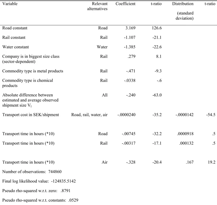
Table 8 presents the best model results from Johnson and de Jong (2011), who use the 2001 Swedish CFS. Their modelling approach is a variant of equation 6.1 and is based on the work of Holguin-Veras (2002). The mean cost and time coefficient have a significant negative effect. Furthermore, the results show significant and substantial unobserved heterogeneity in the cost coefficients and the air-time coefficient. Johnson and de Jong (2011) report that between 5 and 10 per cent of these costs and time coefficients values get a positive sign. The effect V1, which measures the absolute difference between the average and observed shipment for a given mode l and the estimated shipment size, is negative. The implication of this result is that at its average observed shipment size, the capacity of a mode and a shipment
17 Using these results, Windisch (2009) argues that changes in infrastructure that improve shippers’ access to
rail and waterway networks might have a significant effect on decision-making that would result in less road freight transport.
18 As a sensitivity analysis we split the data into domestic and international and applied a mixed MNL model.
22
match very well. When the shipment deviates more from this average (either smaller or larger), the probability of choosing that mode for this shipment will decrease, as implied by the negative sign.
Table 8. Mixed multinomial logit model including estimated shipment size as instrumental variable
Variable Relevant
alternatives Coefficient t-ratio Distribution (standard deviation)
t-ratio
Road constant Road 3.169 126.6
Rail constant Rail -1.107 -21.1
Water constant Water -1.385 -22.6
Company is in biggest size class
(sector-dependent) Rail .279 8.1
Commodity type is metal products Rail -.471 -9.3 Commodity type is chemical
products Rail -.0338 -.6
Absolute difference between estimated and average observed shipment size Vl
All -.240 -63.0
Transport cost in SEK/shipment Road, rail, water, air -.0000240 -35.2 -.0000142 -54.5
Transport time in hours (*10) Road -.00745 -32.2 .0000918 .5
Transport time in hours (*10) Rail -.00317 -17.1 .000132 .5
Transport time in hours (*10) Air -.328 -20.4 .167 19.2 Number of observations: 744860
Final log likelihood value: -124835.5142 Pseudo rho-squared w.r.t. zero: .8791 Pseudo rho-squared w.r.t. constants: .0529
Source: Johnson and de Jong (2011) Table 7.
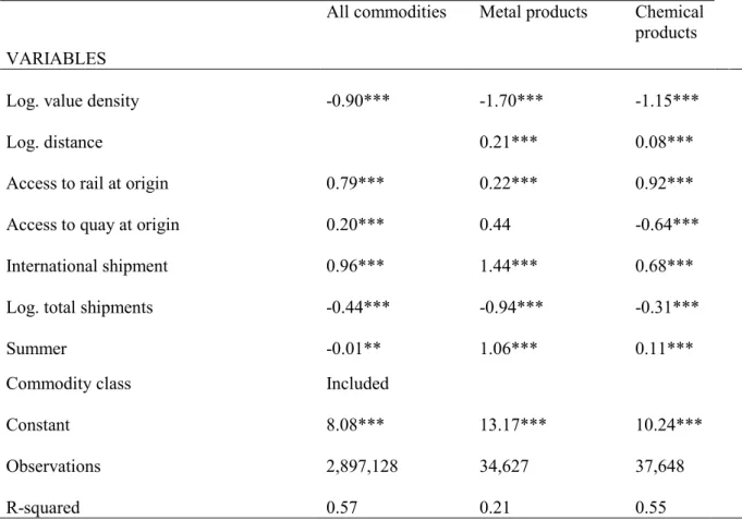
To get insights into what determines shipment size decisions of shippers we estimated equation 6.2 for all commodity groups, metal products, and chemical products. Table 9 presents results from this exercise, where the dependent variable is the log of shipment size.
23
Most of the explanatory variables have expected signs and are statistically significant. As seen from estimates for the value density variable, high value goods are shipped in smaller quantities. The interpretation is that high value products are shipped in smaller quantities, which is generally the case in reality.
For metals products and chemical products, shipments destined for distance places are shipped in larger quantities, as implied by the significant and positive effect of the distance variable coefficients. Shippers who have access to rail or quay at origin ship larger quantities (except chemical product shippers with access to quay at origin). In all three cases, shipments are larger if they are destined for outside Sweden. We found opposite effects for time of year indicator (summer), negative for all commodities and positive for the two commodity groups. Finally, shippers who have a larger number of total shipments per reported period tend to ship in smaller quantities. This result is interesting and reveals the trade-off shippers make between inventory holding and shipment frequency.
Table 9: Independent shipment size model
All commodities Metal products Chemical products
VARIABLES
Log. value density -0.90*** -1.70***
-1.15***
Log. distance 0.21***
0.08*** Access to rail at origin 0.79*** 0.22***
0.92*** Access to quay at origin 0.20*** 0.44
-0.64*** International shipment 0.96*** 1.44***
0.68*** Log. total shipments -0.44*** -0.94***
-0.31***
Summer -0.01** 1.06***
0.11***
Commodity class Included
Constant 8.08*** 13.17*** 10.24*** Observations 2,897,128 34,627 37,648 R-squared 0.57 0.21 0.55 Significance is marked as: *** p<0.01, ** p<0.05, * p<0.1. Source: own estimation
24
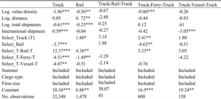
While the results in Table 9 reveal interesting findings on the main determinants of shipment size, the specification they are based on doesn’t take into account the transport mode chain choice problems of shippers. Tables 10 and 11 present a conditional (i.e. conditional on or accounting for transport mode chain choice) shipment quantity models for metal products and chemical products, respectively. The models were estimated using the Dubin-McFadden model that jointly estimates equations 6.1 and 6.2.19 The estimation procedure involves two steps (but estimation is done simultaneously), with the selection probabilities estimated in the first step using equation 6.1. The second step consists of using the estimates from the first step to construct the selectivity correction terms that will be appended to equation 6.2.
Table 10: Conditional shipment quantity model using the Dubin-McFadden Method – metal products
Truck Rail Truck-Rail-Truck Truck-Ferry-Truck Truck-Vessel-Truck Log. value density -1.86*** -0.56** -0.67 -0.86*** -0.26
Log. distance 0.05 0. 72** -2.80 -0.44 -0.83
Log. total shipments -0.61*** -0.25*** 0.25 0.12 .61 International shipment 0.59*** -0.04 -0.27 -0.42 -3.05*** Select_Truck (T) 1.88* 3.14 2.41** 1.80 Select_Rail -3.7*** 1.98 -4.62** -0.51 Select_T-Rail-T 12.37*** 4.36** 3.23** 3.05 Select_T-Ferry-T -4.51*** -1.49** -3.29 -4.22 Select_T-Vessel-T -4.07** -0.51 -2.14 -0.76
Summer Included Included Included Included Included Cargo type Included Included Included Included Included Firm-size Included Included Included Included Included
Constant 10.36*** 6.86** 30.07 16.5*** 19.24**
No. observations 32,348 1,478 43 600 158
Significance is marked as: *** p<0.01, ** p<0.05, * p<0.1. Source: own estimation
19 The STATA ‘selmlog’ command developed by Bourguignon et al. (2007) was used to estimate the two D/C
25
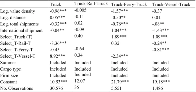
Table 11: Conditional shipment quantity model using the Dubin-McFadden Method – chemical products
Truck Truck-Rail-Truck Truck-Ferry-Truck Truck-Vessel-Truck Log. value density -0.96*** -0.005 -1.57*** -0.37
Log. distance 0.05*** -0.11 -0.50** 0.01
Log. total shipments -0.32*** 0.02 -0.76*** -.08** International shipment -0.04** -0.09 1.04*** -1.43***
Select_Truck (T) 0.40 1.89*** 1.09***
Select_T-Rail-T -8.36*** 0.32 -0.24**
Select_T-Ferry-T -0.45 -0.64 -0.81***
Select_T-Vessel-T 8.92*** 0.34 -2.34***
Summer Included Included Included Included
Cargo type Included Included Included Included Firm-size Included Included Included Included
Constant 10.53*** 12.07 21.79*** 19.18***
No. Observations 30,576 35 5,551 1,486
Significance is marked as: *** p<0.01, ** p<0.05, * p<0.1. Source: own estimation
As seen in Tables 10 and 11, accounting for transport mode chain selection gives different results to those in Table 9 (independent shipment size model). For metal products, although value density has the right negative effect on shipment size for all chains, it is only significant in the ‘Truck’, Rail and ‘Truck-Ferry-Truck’ chains. The effect of distance becomes mixed as well and it is only significant for the ‘Rail’ chain. Similar differences are observed for chemical products as well. These differences are explained by the fact that we now account for the mode chain choice decisions of shippers. The selectivity corrections terms (Select_Truck, etc.) appear to be significant for most chains, implying that the joint estimation procedure is appropriate.
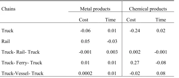
Table 12 reports the marginal effects from the coefficients of the selection models used for the discrete continuous models presented in Tables 10 and 11.20 The estimates indicate the proportional change in the probability of choosing the transport chains for a proportional change in cost and time. Since these are proportional changes, they can be interpreted as elasticities. For metal products, if cost increases (i.e. for all chains) by 10 per cent the demand for Truck and Truck-Rail-Truck chains decreases (relative to the other options) by 6 per cent and 0.1 per cent, respectively. Whereas the demand for Rail, Ferry-Truck and
20The MNL model results on which these marginal impacts are based are not reported, but can be acquired from
the authors upon request. Table A2 in Appendix 2 reports elasticity comparison for three models (similar to the ones presented in this report) conducted by Johnson and de Jong (2011) using the 2001 CFS.
26
Vessel-Truck increases (relative to the other options) by 5 per cent, 1 per cent and 0.02 per cent, respectively. The remaining results are interpreted likewise.
Table 12: Average marginal effects
Chains Metal products Chemical products
Cost Time Cost Time
Truck -0.06 0.01 -0.24 0.02
Rail 0.05 -0.03
Truck- Rail- Truck -0.001 0.003 0.002 -0.001 Truck- Ferry- Truck 0.01 0.01 0.27 -0.08 Truck-Vessel- Truck 0.0002 0.01 -0.02 0.08
V. Conclusions and suggestions for future work
Building on the basic insight that decisions regarding freight transport mode and shipment size are interdependent, in this paper we have reviewed and estimated several econometric models. We have also outlined how results from this exercise could be used as input for updating the Swedish national freight model system (SAMGODS) from its current deterministic version to a stochastic one. The 2004/2005 Swedish National Commodity Flow Survey was used to estimate various models’ specifications at the level of individual shipments. These models simultaneously explain mode and shipment size, where shipment size can be either a discrete or a continuous variable. We have identified that variables such as cost, time, having access to rail or quay at origin and distance are important determinants of shippers’ mode and shipment size choices.
A model in which continuous shipment sizes have been converted into discrete categories produces different behavioural responses to those of the model with continuous shipment size. The latter specification can be seen as the preferred model because it takes account of the endogenous nature of shipment size and uses the shipment size data as they come from the survey. However, applying this model on a large dataset such as the CFS using standard software could be challenging Therefore, in practical applications, a model with two discrete choices might be preferable (see Johnson and de Jong, 2011, for more explanation).
27
Future modelling exercises can extend the models presented here in three important ways. First, there are several individual shipments records in the CFS which were sent by the same shippers. None of the models reviewed and applied here take into account this panel nature of the data. It is, therefore, important to apply models that control for individual (fixed) effects to improve model predictions.
Second, the discrete-continuous models presented here take shipment size as the main variable of interest and are based on selection models estimated by MNL models. While these models are advanced and theoretically sound, practical applications can be problematic. An alternative approach is the discrete-continuous model suggested by Holguín-Veras (2002) (and applied by Johnson and de Jong (2011) on the 2001 CFS, see Table 8). This approach is an interesting one when the main focus is mode choice because it is possible to apply advanced discrete choice models that overcome the independence of irrelevant alternatives (IIA) problem that most selection models suffer from. This approach could be applied on the 2004/2005 CFS, should there be any need of detailed mode choice analysis in the future. Third, more commodity groups (from the 16 sub-groups identified as having potential for change in mode choice) should be studied using the econometric models analysed and suggested here. It is important to take into account as far as possible the logistics structure of shippers of these commodities and the transport network available to them. Generating cost and time variables for CFS shippers has proved to be challenging, mainly due to pitfalls in the CFS (see Appendix 1). These challenges aside, in this project we have generated inputs that could be used for future research and the further development of the national freight model of Sweden.
A general recommendation for future studies is that it is important to make use of existing data sources for scientific and practical modelling purposes. Sweden is one of the very few countries in the world that has detailed micro-level commodity flow surveys. So far, only the 2001 and 2004/2005 Swedish CFSs have been used for scientific studies. To our knowledge, the 2009 CFS is yet be used for scientific purposes. As highlighted in this paper, empirical studies based on the CFS analyse important modelling approaches that could be used as a platform to improve the prediction of national models such as the SAMGODS. It is therefore important to exploit existing data sources and encourage independent empirical modelling efforts. Doing so improves national modelling efforts as well as the scientific literature at large.
28
In addition to helping macro-level modelling efforts, the CFSs could also be used to study micro-level freight demand modelling problems and answer important questions regarding freight movement and infrastructure needs. For instance, using the CFS one can answer questions such: does the length of a highway affect the value and weight of trade between regions in Sweden? And does it affect sectoral specialization of regions in high value/weight sectors? Analyses of the above questions and estimation of the magnitude of such effects provide an important new insight into the way transportation infrastructures affect trade and the organization of economic activity. Better transportation encourages trade in general, and in particular encourages production of and trade in things that are hard to move. In addition to their academic interest, these estimates help inform those involved in designing infrastructure policy. In particular, one can assess the relevant cost-benefit trade-offs involved in the construction of new roads or railways.
29
References
Abate, M. and de Jong, G.C., 2014: The optimal shipment size and truck size choice- the allocation of trucks across hauls. Transportation Research Part A, 59(1) 262–277
Ben-Akiva, M.E. and de Jong, G.C. 2013: The aggregate-disaggregate-aggregate (ADA) freight model system. in: M.E. Ben-Akiva, Meersman, H. and van de Voorde, E., eds. Freight Transport Modelling, Emerald.
Bourguignon, F., Fournier, M., Gurgand, M., 2007. Selection bias corrections based on the multinomial logit model: Monte Carlo comparisons. Journal of Economic Surveys 21 (1), 174–205. de Jong, G.C. and Ben-Akiva, M., 2007: A micro-simulation model of shipment size and transport chain choice. Transportation Research Part B 41(9), 950–965 (2007)
de Jong, G., Ben-Akiva, M., Baak, J., 2010 : Method Report—Logistics Model in the Swedish National Freight Model System (Version 2). Significance, The Hague.
Dubin, J.A. and McFadden, D.L., 1984: An Econometric Analysis of Residential Electric Appliance Holdings and Consumption. Econometrica, 52 (2), pp.345--362.
Habibi, S. , 2010: A Discrete Choice Model of Transport chain and Shipment size on Swedish Commodity Flow Survey, Stockholm: Kungliga Tekniska högskolan, Department of Transport and Logistics.
Holguín-Veras, J., 2002: Revealed Preference Analysis of Commercial Vehicle Choice Process.
Journal of Transportation Engineering, 128 (4), 336--346.
Inaba, F.S. & Wallace, N.E., 1989: Spatial price competition and the demand for freight transportation. The Review of Economics and Statistics, 71 (4), 614--625.
Johnson, D. and de Jong, G.C., 2011: Shippers' response to transport cost and time and model specification in freight mode and shipment size choice. Proceedings of the 2nd International Choice
Modeling Conference ICMC 2011, University of Leeds, United Kingdom, 4 - 6 July.
Liu, X., 2012: Estimating value of time savings for freight transport: a simultaneous decision model of transport mode choice and shipment size. Örebro University Business School, Department of Economics.
Krüger, N; Vierth, I; de Jong, G; Halse A; Killi, M, Value of Freight Time Variability Reductions, VTI-Notat N39-2013 (http://www.vti.se/sv/publikationer/vardet-av-minskad-variabilitet-i-transporttid-for-godstransporter--resultat-framtagen-i-en-pilotstudie-pa-uppdrag-av-trafikverket/)
McFadden, D., Winston, C., and Boersch-Supan, A., 1986: Joint estimation of freight transportation decisions under non-random sampling. In: A. Daugherty, ed. Analytical studies in transport economics. Cambridge University Press, 137--157.
SIKA (2003) Commodity Flow Survey 2001, Method report, SIKA Report 2003:4, SIKA, Stockholm. SIKA ,2004: The Swedish National Freight Model: A critical review and an outline of the way ahead, Samplan 2004:1, SIKA, Stockholm
30
Windisch, E., 2009: A disaggregate freight transport model of transport chain and shipment size choice on the Swedish Commodity Flow Survey 2004/05. MSc Thesis, Delft University of Technology.
Windisch, E., de Jong, G.C and van Nes, R. (2010) A disaggregate freight transport model of transport chain choice and shipment size choice. Paper presented at ETC 2010, Glasgow