Groundwater modelling for monitoring purposes in construction projects
15
0
0
Full text
(2) Miracapillo. C.. In order to interpretate the collected data, a groundwater simulation model is built up and used for the following purposes : - to calculate the flow field and the fluxes - to calculate the area of influence of some pumping wells, which happened to be contaminated during the construction phase - to simulate the transport of contaminants, which could be present in the area of influence of the pumping wells - to evaluate the efficiency of the remediation measures The aim of this article is to focuse attention on a quantitative evaluation of the impact of the construction on the groundwater flow showing the results of the numerical model in terms of flow field and water fluxes.. 2. The project area and the project This article refers to a road construction project in the city of Basel in Switzerland. The project area is a quarter of Basel, on the right-hand side of the Rhein. Important hydrological components are the Rhein, which act as a receiving stream, and the river Wiese, an affluent of the Rhein, which flows north of the construction site. The geological formation is the result of two fluvial deposits, the Rhein and the Wiese deposits. The deposits consist of gravel and sand of different grain size. The groundwater direction is EastWest. The project is proportioned in several stretches. The one considered here involves the construction of underground structures underneath the water table. There, the water table is drawn down to a prescribed level using 51 pumping wells around the construction site. The total pumping rate varies during the construction phase (1997-1990) and reaches the maximum value of 183 l/sec in April 98.. 3. The numerical model In order to quantify the impact of the construction, a 2-D Model is developed using the numerical code ASM (Aquifer Simulation Model) based on the finite Difference Method. The model area (3.7 km2) covers a part of a quarter of Basel located along the Rhein. The groundwater flows in undisturbed conditions under low hydraulic gradients into the Rhein perpendicular to the river bank. It is realistic to assume that the Rhine and the aquifer are in hydraulic connection. The Rhein at the west boundary of the model area is the outflow boundary ( Fig.1). The east boundary is the inflow boundary. West and East boundaries are simulated with boundaries conditions of the first order using respectively the water level in the Rhein (west boundary) and the available piezometer levels (east boundary). The north and south boundaries of the model area are built up with boundary conditions of the second order (streamlines). The Wiese is simulated with third order boundary conditions (leakage). The model area is discretized in cells whose size varies from 20m×20m to 5m×5m close to the construction site.. 168.
(3) Groundwater modeling for monitoring purposes in construction projects. Inflow (river Wiese). Ou tf (Zo low ne3 ). Inflow (Zone 1). Rhein. Wiese. low I nf e 2 ) n (Zo. construction site. Zone 1 Yellow 2 Brown 3 Pink 4 Red 5 Green. low Outf 5) e (zon. monitoring Station. Fig.1 – The model area: the inflow and outflow components Zone 1 = Inflow north of the Wiese Zone 2 = Inflow south of the Wiese Zone 3 = Outflow north of the Wiese Zone 4 = Outflow south of the Wiese, north of the axes of the road construction Zone 5 = Outflow south of the Wiese, south of the axes of the road construction. 4. Data Based on pumping tests carried out in a zone close to the model area, the hydraulic conductivity of the aquifer is estimated to be between 1mm/s and 3 mm/s. As a result of the model calibration it is found that the value of 1.7 gives the best matching between calculated and measured piezometer levels at 19 stations. The effective porosity was assumed to be 15 %. For the 169.
(4) Miracapillo. C.. leakage coefficient of the river Wiese, the value of 9·10-6 s-1 was assumed, according to previous experiences. The water level in the Wiese and in the Rhein varies from one Scenario to another according to the hydrological data. The piezometer values and pumping rate of private wells located in the model area are provided by the AUE (Amt für Umwelt und Energie), the hydrological data by BWG (Bundesamt für Wasser und Geologie) and project layout and the characteristics of the construction site and of the drainage system are provided by the contractor and TBA (Tiefbauamt). The aquifer bottom is obtained from an interpolation code using data from existing boreholes (Databank of the Kantonsgeologie Basel-Stadt) (Fig.2).. Aquifer bottom Yellow 233.3 - 236.5 m a.s.l. Blue 236.5 - 239.5 m a.s.l. Green 239.5 - 242.5 m a.s.l.. Piezometer. Fig.2 – The aquifer bottom. 5. The scenarios The groundwater model allows to calculate the flow field and the fluxes for the entire model area and for the zone previously defined. Calculations are carried for three situations, namely, the situations before, during and after construction, which are chosen as representative of the undisturbed situation, of the strongest impact during the construction phase and of the long term impact after construction, respectively. The numerical simulations are made under stationary conditions. 170.
(5) Groundwater modeling for monitoring purposes in construction projects. The choice of the data set which could adequately represent the situations before and after construction depends on the availability of data and is based on stationary pumping rates at the construction site and on stationary hydrological conditions. This is the case in May 1997 (before construction) and December 1999 (after construction). The data sets refer to monthly mean values. The data set which represents the situation during construction (April 1998) corresponds to the phase of the maximum aquifer draw down and the biggest value of the total pumping rate. The data set refers to daily mean values. In the three scenarios the water level in the Rhein varies between 244.1 and 244.6 m a.s.l. and the water level in the Wiese varies between 20 and 50 cm above the river bed.. Zon e 1,5 3: l/s. Zone 1: 82 l/s. Zone 4: 19 l/s 2: ne Zo l/s 8 6. 8 24. 7 24. 5: Zone /s 24 p. 6 24. 5 24. hmin = 244.5 m a.s.l. hmax = 249 m a.s.l. ∆h = 0.5 m. Fig.3 – Undisturbed situation: groundwater flow field and piezometer levels (Calibration May 1997). 171.
(6) Miracapillo. C.. 6. The situation before construction The situation before construction is simulated by the model calibrated upon the data set of May 1997. This situation represents the undisturbed case. Fig.3 shows the groundwater flow field, the piezometer levels, the groundwater inflow and outflow components, as they result from the water budget over the defined zones.. 7. The situation during construction During the construction phase the impact is due to the underground structures (temporary and permanent) and to the pumping at the construction site. The walls of the construction site are made using two different systems: Lamella wall to the bottom of the construction site and bore piles with different penetrating depth into the aquifer and sometimes to the aquifer bottom. Two kinds of bore piles (Fig. 4) are used: -Bore piles (with and without reinforced concrete and of different lengths) -Bore piles with an opening ( a moving element or slide allows the water to flow through) The openings are kept closed during the construction phase.. Permeable grevel. Bore piles made of concrete. Piezometer. Pile with opening. Bore piles made of reinforced concrete. Pile with openings. Fig.4 – The wall at the construction site: bore piles made of concrete, bore piles made of reinforced concrete, bore piles with slides ( Mitt. Schweiz. Ges. f. Boden - u. Felsmechanik, 1996) In this case the walls are simulated using an equivalent K-value Ke for the corresponding cells (Fig.5), namely Ke = c·K where c = H0/Htot being K the hydraulic conductivity of the model area, H0 the free depth under the piles or the walls and Htot the total depth in aquifer. 172.
(7) c = 0.3. c = 0.6. c = 0.2. c = 0.4 c=0 c = 0.5. c = 0.3. c = 0.1 c = 0.35. c=0. c = 0.2. c = 0.4. c = 0.3. Groundwater modeling for monitoring purposes in construction projects. Piezometer. Fig.5 - Coefficients c to calculate Ke for the simulation of the construction site The underground constructions which reach the aquifer bottom are simulated with impermeable cells (inactive cells). The groundwater flow field is shown in Fig.6. The resulting components, calculated with the water budget, are also shown.. 8,3 l/s. 78 l/s. 27 l/s. l/s 73. 8 24. 7 24. 6 24. 8 l/s. 5 24. hmin = hmax = ∆h =. 238 m a.s.l. 249 m a.s.l. 0.5 m. Fig.6 – The situation during construction: groundwater flow field and piezometer levels (Calibration April 1998). 173.
(8) Miracapillo. C.. 7. The situation after construction The impact on the groundwater flow is due to the underground constructions like walls, piles, foundations which permanently remain in the aquifer after the construction phase. The openings of the piles with slides allow the water to flow trough in the direction perpendicular to the axes of the construction site. The openings are considered as an additional free space (every 5.25 m) to the free depth. The numerical simulation is carried out under the assumption that all the slides can be opened. The simulation results in this case are shown in Fig.7. Zon e 1, 2 3: l/s. Zone 1: 58 l/s. Zone 4: 16 l/s 2: ne Zo 0 l/s 5. 7 24. 6 24. 5: Zone /s 14 p. 5 24. hmin = hmax = ∆h =. 243.5 248 0.5. m a.s.l. m a.s.l. m. Fig.7 – The situation after construction: groundwater flow field and piezometer levels (Calibration December 1999) An additional simulation is made with the data set of December 1999 and without the construction site. The results (in terms of piezometer levels and components of the water budget) are exactly the same as in the above scenario. 174.
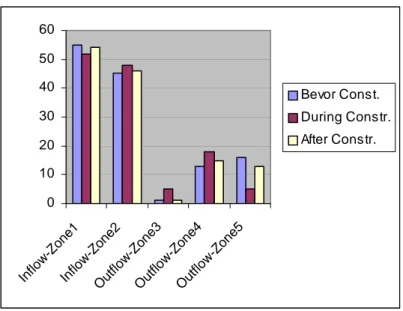
(9) Groundwater modeling for monitoring purposes in construction projects. 8. Results The scenarios are calibrated upon the piezometer levels measured at 19 monitoring stations. The best agreement between data and numerical results is found for the calibration of December 1999. In this case the assumption of stationary conditions is better supported by the data, which remain almost constant during December 1999. The difference between measured and calculated piezometer levels do not exceed 20 cm. The only exception is the Piezometer 718. There the error is of 40 cm. Quite a good agreement show the calibration of Mai 1997 and April 1998. There the only exception is the Piezometer 752 with an error of around 80 cm between calculated and measured values. The standard deviation is calculated disregarding the two piezometers (718 and 752) since they give unexpected value and they are not directly located in the zone of interest. The Results are: Calibration Situation before construction Situation during construction Situation after construction. Standard Deviation 0.29m 0.28m 0.11m. In order to evaluate the changes in the underground water circulation, the inflow and outflow in defined subregions (s. Fig.1) are determined and plotted in Fig.8 (as absolute values) and in Fig.9 (as percentage of the groundwater total inflow). 90 80 70 60 50 40 30 20 10 0. Bevor Const. During Constr.. -Z O on ut e2 flo w -Z O on ut e3 flo w -Z O on ut e4 flo w -Z on e5. w flo In. In. flo. w. -Z on. e1. After Constr.. Fig.8 – Groundwater inflows and outflows (l/s) in defined subregions for different Scenarios. 175.
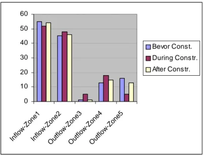
(10) Miracapillo. C.. 60 50 40. Bevor Const.. 30. During Constr.. 20. After Constr.. 10. on e2 flo w -Z O on ut e3 flo w -Z on O ut e4 flo w -Z on e5. O ut. w flo In. In f. lo w. -Z. -Z. on. e1. 0. Fig.9 – Inflows and outflows as a percentage of the total groundwater inflow The study of the groundwater flows confirms the higher impact of the project in the construction phase compared to the situation after construction. The total groundwater inflow is almost the same for the situation before and during construction (150 l/s) and smaller in the situation after the construction site (108 l/s). The analysis of the flow components as percentage of the total inflow shows that the impact of the construction on a regional scale is not relevant and that the pumping at the construction site modify the outflows from the model area, namely the infiltration in the Rhine. The Wiese is also an important hydrological component. Infiltration and exfiltration are possible depending on the hydrological conditions and on the pumping rate at the construction site and on the pumping rate in the wells located near the river. The inflow and outflow are plotted in fig.10. 0.1 0.09 0.08 0.07 0.06. Wiese Inflow. 0.05. Wiese Outflow. 0.04. Inflow-Outflow. 0.03 0.02 0.01 0 Bevor Const.. During Constr.. After Constr.. Fig. 10 – Wiese inflow and outflow (m3/s) for different Scenarios 176.
(11) Groundwater modeling for monitoring purposes in construction projects. 8. The situation after construction The impact on the groundwater flow is due to the underground constructions like walls, piles, foundations which permanently remain in the aquifer after the construction phase. The openings of the piles with slides allow the water to flow trough in the direction perpendicular to the axes of the construction site. The openings are considered as an additional free space (every 5.25 m) to the free depth. The numerical simulation is carried out under the assumption that all the slides can be opened. The simulation results in this case are shown in Fig.7. Zon e 1, 2 3: l/s. Zone 1: 58 l/s. Zone 4: 16 l/s 2: ne Zo 0 l/s 5. 7 24. 6 24. 5: Zone /s 14 p. 5 24. hmin = hmax = ∆h =. 243.5 248 0.5. m a.s.l. m a.s.l. m. Fig.7 – The situation after construction: groundwater flow field and piezometer levels (Calibration December 1999) An additional simulation is made with the data set of December 1999 and without the construction site. The results (in terms of piezometer levels and components of the water budget) are exactly the same as in the above scenario. 177.
(12) Miracapillo. C.. 9. Results The scenarios are calibrated upon the piezometer levels measured at 19 monitoring stations. The best agreement between data and numerical results is found for the calibration of December 1999. In this case the assumption of stationary conditions is better supported by the data, which remain almost constant during December 1999. The difference between measured and calculated piezometer levels do not exceed 20 cm. The only exception is the Piezometer 718. There the error is of 40 cm. Quite a good agreement show the calibration of Mai 1997 and April 1998. There the only exception is the Piezometer 752 with an error of around 80 cm between calculated and measured values. The standard deviation is calculated disregarding the two piezometers (718 and 752) since they give unexpected value and they are not directly located in the zone of interest. The Results are: Calibration Situation before construction Situation during construction Situation after construction. Standard Deviation 0.29m 0.28m 0.11m. In order to evaluate the changes in the underground water circulation, the inflow and outflow in defined subregions (s. Fig.1) are determined and plotted in Fig.8 (as absolute values) and in Fig.9 (as percentage of the groundwater total inflow). 90 80 70 60 50 40 30 20 10 0. Bevor Const. During Constr.. -Z O on ut e2 flo w -Z O on ut e3 flo w -Z O on ut e4 flo w -Z on e5. w flo In. In. flo. w. -Z on. e1. After Constr.. Fig.8 – Groundwater inflows and outflows (l/s) in defined subregions for different Scenarios. 178.
(13) Groundwater modeling for monitoring purposes in construction projects. 60 50 40. Bevor Const.. 30. During Constr.. 20. After Constr.. 10. on e2 flo w -Z O on ut e3 flo w -Z on O ut e4 flo w -Z on e5. O ut. w flo In. In f. lo w. -Z. -Z. on. e1. 0. Fig.9 – Inflows and outflows as a percentage of the total groundwater inflow The study of the groundwater flows confirms the higher impact of the project in the construction phase compared to the situation after construction. The total groundwater inflow is almost the same for the situation before and during construction (150 l/s) and smaller in the situation after the construction site (108 l/s). The analysis of the flow components as percentage of the total inflow shows that the impact of the construction on a regional scale is not relevant and that the pumping at the construction site modify the outflows from the model area, namely the infiltration in the Rhine. The Wiese is also an important hydrological component. Infiltration and exfiltration are possible depending on the hydrological conditions and on the pumping rate at the construction site and on the pumping rate in the wells located near the river. The inflow and outflow are plotted in fig.10. 0.1 0.09 0.08 0.07 0.06. Wiese Inflow. 0.05. Wiese Outflow. 0.04. Inflow-Outflow. 0.03 0.02 0.01 0 Bevor Const.. During Constr.. After Constr.. Fig. 10 – Wiese inflow and outflow (m3/s) for different Scenarios 179.
(14) Miracapillo. C.. The ratio between infiltration and exfiltration in both situations before and after construction is between 4 and 5, while during construction the river practically only infiltrates. The infiltration rate during construction is twice bigger than before construction. The plot shows also a higher infiltration rate after construction than before construction. This is related to the hydrological data set of the calibration of December 1999 (lower groundwater inflow and lower groundwater levels). Under the same hydrological conditions the terms are very similar.. 10. Conclusions Constructions underneath the water table involving the drawing down of the water table to a prescribed level modify the flow field. In order to evaluate the impact of the construction on the groundwater system a monitoring program was carried out and a numerical model was developed. A correct statement of the problem would imply calculations of the flow field under transient conditions and a 3-D simulation of the construction site and of the aquifer. For the sake of simplicity an alternative way is followed. The transience of the real situation is replaced through the simulation under permanent conditions of three situations, namely, the situations before, during and after construction. These are chosen as representative of the undisturbed situation, of the strongest impact during the construction phase and of the long term impact after construction, respectively. The geometric characteristics in the vertical direction of the walls at the construction site are taken into account in a approximate way with a reduction of the hydraulic conductivity. The procedure is accurate enough. The standard deviations calculated for each situation show that the numerical results are in good agreement with the data. It is also clear that the axes of the construction site and the direction of the groundwater flow play an important role. Here the axes of the road is approximately parallel to the flow direction and the impact of the underground construction is not relevant on a regional scale. The analysis of the components of the water budget confirms that the impact of the construction on the groundwater system has only local effects. The groundwater flow field results show a shift of the piezometer level between the north and south sites of the construction site and correspond to around 20 cm. It is not excluded that the real impact of the underground structures is locally higher, depending on the percentage of the slides by the bore piles which can be opened successfully at the end of the construction. Acknowledgement. Part of this study was made during the collaboration of the author as researcher and lecturer with the group of Applied Geology at the Geological Institute of the University of Basel. The author would like to acknowledge the guidance of Prof. P. Huggenberger and the useful discussions with his group. The author would like also to acknowledge also the collaboration with the GI (Geotechnical Institut in Basel, Dr. B. Vögtli) for leading the groundwater monitoring program in the project area. The support of the AUE (Amt für Umwelt und Energie, Baselstadt, R. Neher) was 180.
(15) Groundwater modeling for monitoring purposes in construction projects. precious for providing and interpreting the data. In addition, the financial and technical support of the TBA (Tiefbauamt Baselstadt, Nationalstrassenbüro, J. Renz and Ch. Angst) was essential for the good results of this study.. Bibliography Groundwater management in the region of Basel, P.Huggenberger, C. Miracapillo and Ch. Regli, Lecture in NDK in angewandten Erdwissenschaften, 18. Blockkurs, 24-29September, 1991, Kurszentrum Schloss Münchenwiler N2 Nordtangente, Abschnitt 4: Horburg, Grundwasserüberwachung Erfolgskontrolle, Report, J.Renz, P.Huggenberger, C.Miracapillo, R.Neher, R.Studer, D.Gysin, M.Brunkhorst Wegleitung zur Umsetzung des Grundwasserschutzes bei Untergebauten, Buwal 1998 Mitt. Schweiz. Ges. f. Boden - u. Felsmechanik, 1996. 181.
(16)
Figure
Related documents
The increasing availability of data and attention to services has increased the understanding of the contribution of services to innovation and productivity in
Av tabellen framgår att det behövs utförlig information om de projekt som genomförs vid instituten. Då Tillväxtanalys ska föreslå en metod som kan visa hur institutens verksamhet
Närmare 90 procent av de statliga medlen (intäkter och utgifter) för näringslivets klimatomställning går till generella styrmedel, det vill säga styrmedel som påverkar
I dag uppgår denna del av befolkningen till knappt 4 200 personer och år 2030 beräknas det finnas drygt 4 800 personer i Gällivare kommun som är 65 år eller äldre i
Den förbättrade tillgängligheten berör framför allt boende i områden med en mycket hög eller hög tillgänglighet till tätorter, men även antalet personer med längre än
På många små orter i gles- och landsbygder, där varken några nya apotek eller försälj- ningsställen för receptfria läkemedel har tillkommit, är nätet av
DIN representerar Tyskland i ISO och CEN, och har en permanent plats i ISO:s råd. Det ger dem en bra position för att påverka strategiska frågor inom den internationella
Indien, ett land med 1,2 miljarder invånare där 65 procent av befolkningen är under 30 år står inför stora utmaningar vad gäller kvaliteten på, och tillgången till,
