Railway Power Supply Models and Methods for Long-term Investment Analysis

LARS ABRAHAMSSON

Licentiate Thesis Royal Institute of Technology School of Electrical Engineering

Electric Power Systems Stockholm, Sweden, 2008

TRITA-EE 2008:036 ISSN 1653-5146

ISBN 978-91-7415-083-4

Royal Institute of Technology SE-100 44 Stockholm Sweden Akademisk avhandling som med tillstånd av Kungl Tekniska högskolan framlägges till offentlig granskning för avläggande av teknologie licentiat-examen fredagen den 5:e september 2008 kl. 10.00 i sal V32, Teknikringen 72, Kungl Tekniska Högskolan, Stockholm.

© Lars Abrahamsson, augusti 2008 Tryck: Universitetsservice US-AB

The aim of the project is to suggest an investment planning program where the welfare of the society is to be maximized. In order to be able to decide on a wise investment plan, one needs to know the consequences of different choices of power system configurations. Therefore the impacts of different future traffic demands are of interest for a railway power system owner.

Since investments are supposed to last a long time, their future usage has to be considered. Moreover, the lead times of investments can be of considerable duration lengths. Because of the uncertainty of the future, deterministic case studies might not be suitable and then a large number of outcomes are to be studied, probable outcomes as well as outcomes with a high level of impact.

In order to be able to make a valid long-term investment analysis of the railway power supply system, one needs to use proper railway power supply models and methods. The aim of this thesis is to present a stable modeling and methodological basis for the coming investment planning phase of this PhD research project. The focus is set on studying the consequences of a railway power supply system which is too weak.

The thesis contains an overview of models of some electrical and me-chanical relations important for electric traction systems. Some of these models are further developed, and some are modified for improved compu-tational properties. A flexible electric traction system simulator based on the above mentioned models has been developed and the applied methods and resulting abilities are presented.

The main scientific contribution of this thesis is that a fast and approx-imative neural network model, which calculates some important aggregated results of the interaction between the railway power system and the train traffic, has been developed. This approximative model was developed in order to reduce computation times. Reduction of computation times is very

important when a huge number of outcomes are studied. A complete sim-ulation of a train power system in operation takes a long time, often not less than about a tenth of the simulated traffic time. The neural network is trained with some selected aggregated results extracted from a wide set of railway operation simulation cases. The choices of network inputs and outputs are motivated in the thesis. The performance of the simulator as well as the approximator are visualized in case studies.

Syftet med projektet är att föreslå ett investeringsplaneringsprogram där något slags välfärdsmått skall maximeras. För att kunna besluta sig för en bra investeringsplan måste man känna till konsekvenserna av olika val av strömförsörjningstekniker. Därför är inverkan av olika framtida trafikbehov av intresse för en ägare till ett järnvägselsystem.

Eftersom investeringar antas bestå en längre tid, måste hänsyn tas till deras framtida användning. Vidare kan investeringarnas ledtider vara långa. På grund av den osäkra framtiden, kan det hända att deterministiska fall-studier inte är lämpliga. Ett sätt att hantera osäkerheterna är att studera en stor mängd utfall, troliga utfall såväl som utfall med stor inverkan på resultaten.

För att kunna göra en giltig långtidsinvesteringsanalys av järnvägens strömförsörjningssystem måste man använda korrekta modeller och metoder för järnvägselsystemet. Syftet med avhandlingen är att presentera en stabil modellerings- och metodikgrund att stå på i den kommande investerings-planeringsfasen i detta doktorandprojekt. Fokus är inställt på att studera konsekvenserna av ett elsystem som är för svagt för att försörja järnvägen med tillräckliga mängder ström.

Avhandlingen innehåller en översikt av modeller av några elektriska och mekaniska samband som är viktiga för eldriven spårtrafik. Några av dessa modeller är också vidareutvecklade, och några är modifierade för att förbät-tra deras beräkningsmässiga egenskaper. En flexibel simulator för eldriven spårtrafik som bygger på ovan nämnda modeller har utvecklats och de an-vända metoderna samt simulatorns prestanda presenteras i avhandlingen.

Det huvudsakliga vetenskapliga bidraget i avhandlingen är att en snabb och approximativ neural nätverksmodell som beräknar vissa viktiga ag-gregerade resultat från interaktionen mellan järnvägselsystemet och tåg-trafiken har utvecklats. Denna approximativa modell utvecklades för att

kunna reducera beräkningstiderna. Reduktion av beräkningstider är myck-et viktigt när en myckmyck-et stor mängd utfall skall studeras. En fullständig simulering av ett järnvägselsytem i drift tar lång tid, oftast inte mindre än ungefär en tiondel av den simulerade trafiktiden. Parametrar för det neurala nätverket har erhållits genom att träna det med några utvalda aggregerade resultat uttagna från en stor mängd av simulerade järnvägsdriftsfall. Valen av nätverksinputs och -outputs motiveras i avhandlingen. Såväl simulatorns som approximatorns prestationsförmågor visualiseras med hjälp av fallstudi-er.

First, I would like to thank my supervisor, Professor Lennart Söder, for his supervision of and patience with the work I have done, and of course also for initiating this research project together with Sam Berggren, Banverket, the Swedish state-owned railway administrator.

Moreover, thanks go to Elektra for financing the research project. I would also like to thank the members of the steering committee of my project: Anders Bülund, Viktoria Neimane, and Thorsten Schütte for their experience, knowledge and ideas.

Finally, I would like to thank my fellow PhD students and other col-leagues at the division of Electric Power Systems, KTH, for making the coffee and lunch breaks pleasant. Katherine Elkington deserves mentioning by name thanks to her LA_{TEX support.}

Contents ix

1 Introduction 1

1.1 Background . . . 1

1.2 Aim, Main Assumptions and Limitations. . . 3

1.3 Main Contribution . . . 5

1.4 Outline . . . 6

1.5 List of Publications . . . 7

2 Power Supply of Railways and its Models 9 2.1 Background material . . . 10

2.1.1 In General . . . 10

2.1.2 Expansion planning of the railway power supply system 10 2.1.3 Operation costs of the railway power supply system . 11 2.1.4 Other Railway Research . . . 13

2.2 Nomenclature . . . 14

2.3 Conductors and their models . . . 14

2.3.1 Catenary . . . 14

2.3.2 Transmission Line . . . 19

2.3.3 The modeled power line impedances in the context of the power supply system . . . 20

2.4 The Frequency Converters . . . 21

2.4.1 Background . . . 21

2.4.2 Models . . . 24

2.5 Locomotives and Trains . . . 26

2.5.1 Introduction . . . 26 ix

2.5.2 Common Models for Tractive Force and Tractive

Power Limits and Regulation . . . 27

2.5.3 The Electrical and Mechanical Power Consumption Models used in this Thesis . . . 31

2.5.4 Train Braking Model . . . 38

2.6 Capacity Limits in Electric Equipment . . . 41

2.7 Strengthening of the Railway Power Supply . . . 42

2.8 Reliability . . . 43

2.9 Capacity . . . 43

3 The Simulator 45 3.1 Aim of, and Motivation for TPSS . . . 45

3.2 A Review of Existing Railway Power Supply System Simulators 46 3.2.1 OpenPowerNet . . . 46

3.2.2 SIMON . . . 47

3.2.3 A Probabilistic Load Flow Approach . . . 48

3.2.4 Some other railway power system software . . . 49

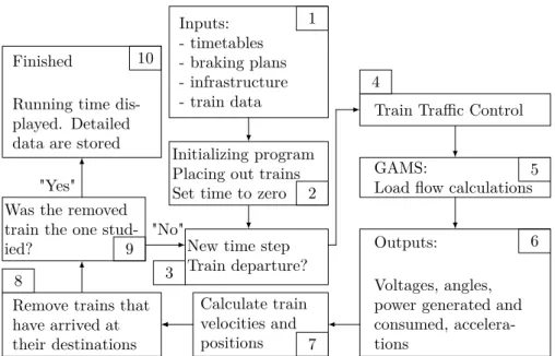
3.3 The Method of TPSS . . . 50 3.3.1 Flowchart . . . 50 3.3.2 A General Description . . . 50 3.3.3 A Detailed Description . . . 54 3.4 Possible Improvements . . . 69 3.5 Case Studies . . . 70 3.5.1 Simulation Results . . . 71

3.5.2 Future Case Studies . . . 80

4 The Approximator 81 4.1 A motivation for the development of the TPSA . . . 81

4.1.1 Investment Planning for Power Systems . . . 81

4.1.2 The Necessity for a Fast Approximative Model for Long-term Planning . . . 81 4.1.3 Background . . . 83 4.1.4 Remarks . . . 84 4.2 Related Work . . . 85 4.3 Model . . . 86 4.3.1 A Short Background . . . 86

4.3.2 The TPSA Model . . . 87

4.3.4 Neural Network . . . 91

4.4 Numerical Example . . . 94

4.4.1 Problem Setup . . . 94

4.4.2 Numerical Results . . . 95

4.5 Conclusion and Summary . . . 104

4.6 Future Work . . . 104

4.6.1 Time-continuous Traffic . . . 104

4.6.2 Development of TPSS . . . 105

4.6.3 Better and Accessorial Simulation Data . . . 105

4.6.4 Development of TPSA . . . 106

5 Conclusions and Future Work 109 5.1 Conclusions . . . 109

5.2 Further Work . . . 110

5.2.1 Improvement of Work Presented in this Thesis . . . . 110

5.2.2 Post-licentiate Work . . . 110

A Neural Networks 113 B Models for Tractive Force Curves 117 B.1 Maximal Short-Time Tractive Force . . . 117

B.1.1 Layer 1, hidden, tansig transfer functions . . . 117

B.1.2 Layer 2, output, linear transfer functions . . . 118

B.2 Maximal Continuous Tractive Force . . . 119

B.2.1 Layer 1, hidden, tansig transfer functions . . . 120

B.2.2 Layer 2, output, linear transfer functions . . . 120

C The Double Arc Curve 123 D Scaling of the Locomotive DC Voltage 125 E Numerical Data Used in TPSS 127 F A skeleton model of an extended TPSA 135 F.1 Possible TPSA Inputs . . . 138

F.2 Possible TPSA Outputs . . . 141

Introduction

1.1

Background

For more than a decade, the railway has in many countries experienced a renaissance after several decades of decay. The main reasons for the renewed interest in the railway are environmental, economical, and safety related. This has quite naturally, in turn, increased the interest in railway associated research.

Both personal and goods transports on railway are increasing. This is not an increase only in the number of departures, but also heavier trains for goods, and faster trains for personal transports. In order to cope with this increase, large railway infrastructure investments are expected. An important part of this infrastructure is the railway power supply system – without it, only the weaker and less energy efficient [100] steam and diesel locomotives could be used.

When making a decision about the future railway power supply sys-tem, the costs for possible under-investments or over-investments need to be estimated in an appropriate manner. The costs of over-investments are the difference between the investment cost of the "too strong" and the cost for a "sufficiently strong" power system configurations. Costs that are re-lated to under-dimensioning are similarly the investment cost of a power system which is too weak, plus the additional operation costs related to its weakness, minus the investment cost of the "sufficiently strong" power system. Since some of the operation costs are hard to value monetarily, an exact definition of "sufficiently strong" does not really exist. Some

tant under-dimensioning costs are described and compared to the case of a public electric power system in the following paragraph:

An under-dimensioned power system, i.e. an electric power system which is too weak, is in general characterized by substantial voltage drops when stressed. Whereas a voltage drop in the ordinary public power system would cause occasional disconnections of customers, it would only cause the trains to run slower in the power supply system of the railway. This can be ex-plained by the fact that the power customers of the railway are less fastidious than those of the public power grid. Moreover, short-time interruptions or outages can be costly in the public power system whereas in the railway power supply system they are in theory nearly not noticed, thanks to the great momentum of a train set at high speed. In reality however, due to safety reasons, trains slow down at outages.

In order to be able to monetarily value every combination of power sys-tem configuration and traffic demands, one has to assume that most indirect results of decisions taken that affect the state of the power system, including e.g.

• Scheduled train running time lengths

• Train delays, i.e. when the actual running times exceed the scheduled running times

• Environmental impacts depending on peoples choices of means of transportation

• Socioeconomic gains for widened labor market regions,

can be modeled as monetary gains or costs. If the low capacity of a power supply system is already accounted for during the construction of the timetable, the costs relate only to the reduced competitiveness on the transportation market. If, on the other hand, the delay time is underesti-mated or not even accounted for by the designer of the timetable, the costs will also include disturbed, or even modified, timetables. In worse cases, the latter may lead to possibly canceled trains, and if it happens often, in bad will for the entire railway sector.

With the trend of increasing energy prices and the environmental im-pact of wasting energy in mind, power consumption, including losses, is also an important parameter to study, when planning the future power supply system. The studies of power consumption will also be helpful when placing

the converter stations and distributing the converters between the converter stations. The determination of converter station capacities is important, be-cause it is desirable to transport power over as short distances as possible on the overhead contact wire, called the catenary. The possible choice between power transmission in 50 Hz high voltage lines, through transformers and converters, or in 16.7 Hz high voltage lines, through transformers, depends much on the local prerequisites.

A slightly under-dimensioned power supply system might lead to higher energy consumption because of increased losses, whereas a severely under-dimensioned system would hardly allow the trains to consume any power at all.

1.2

Aim, Main Assumptions and Limitations.

The aim of the entire PhD project is to suggest an investment planning program where the welfare of the society is to be maximized, or equivalently, some socioeconomic cost is minimized. The program will take into account the fact that the investment decisions for the power supply system of the railway are being made by a national administrator.

The aim of this thesis is to set up a stable modeling and methodolog-ical ground to stand on in the coming investment planning phase of this PhD research project. The focus is set on studying the consequences of a railway power supply system which is too weak. This is done in order to make it possible to formulate a socioeconomic investment planning problem, maximizing the welfare of the society. It is nontrivial to know exactly how much, when and where the traffic will increase. This leads to investment planning for an uncertain future. When studying an uncertain future with many different decisions to be made at several possible moments in time, it is suitable to study many cases. A proper railway power system simu-lation consumes a lot of time. In order to keep the computation-times of the planning-program manageable, some simplifications have to be made, with the most interesting relations preserved. This altogether motivates the suggested neural network approximator.

Today in Sweden, traffic forecasts are first determined by the mar-ket/society division of the railway administrator. These forecasts are then used for timetable construction with the maximization of some socioeco-nomic utility as objective. The timetables constructed are later used when

simulating future railway traffic for determining exactly which investments should be made in the power system [30, 81, 114]. In the planning process, the infrastructure, including rail, power supply, or other things, is normally treated on a higher level of abstraction [39]. This research project aims to include some more details about the power supply system investment plan-ning into the entire planplan-ning process. Such details include, e.g. the choice of catenary type, the possible usage of high voltage lines, the capacity of each converter station, and the inter-converter-station distances.

The Train Power System Simulator (TPSS) presented in this thesis is a computer program that simulates train movements and their interaction with the electric power supply system of the railway over time. TPSS con-siders the electric power consumption characteristics of the locomotives; the impedances of catenary lines, High Voltage (HV) lines, and transformers; the nonlinear relations of voltages and power flows that describes the long-term, i.e. the steady state, behavior of the frequency converters of the railway; the track topographies, i.e. a forward-pushing force when going downhill, and conversely, a counter-force when going uphill; the resistive forces of moving trains excluding gravitation; speed limitations; and times needed for brak-ing. The models used in TPSS treats the connections to the 50 Hz power system as infinite buses supplying the frequency converters with power. In-puts to TPSS is the desired train traffic timetable including train types, the power system configuration, the desired time step length of the simulator, the track topography, and speed limits. The TPSS outputs are the state of the power system, i.e. the voltage levels and angles in all nodes; the amount of generated active and reactive power on the 16.7 Hz side of the converters; and the consumed active and reactive power of the locomotives; and the positions, velocities, and accelerations of every train; for every time step simulated.

Moreover, in order to avoid time demanding simulations in the phase of expansion planning, a simplified model denoted TPSA (Train Power System Approximator) has been developed. TPSA is given a compact description of a certain section of an electric feeding system, a certain level of train traffic there, and gives out the performance of this certain combination. In other words, the inputs and outputs are of the same kinds as for TPSS, but in an aggregated form. TPSA is developed as a neural network. The inputs and outputs of TPSA are of the kind that are judged to be important for railway power supply system expansion. In stochastic optimization, a tremendous number of situations have to be considered. That fact motivates

the desire to study each situation in a relatively fast way. TPSA should be trained with a sufficient number of simulation results, or rather, if avail-able, measurement data, to give realistic output results for un-simulated, or unmeasured, situations that are likely to occur. It should be pointed out, that the approximator also should give reasonable output results for traffic situations that only seldom can occur in the reality.

Limitations in the in this thesis presented simulator models are

• No attention has been paid to protection systems and electrical break-ers this far.

• The train driver behavior is simplified.

• Auxiliary power needs are neglected, only tractive power is studied in detail.

• Power losses in locomotives and power converters are not considered. • Overheating of equipment is not considered.

• The signaling system has this far been disregarded in the study. • Harmonics are not considered in this thesis, but models can be found

in [97].

• Purely static power system models are used, i.e. all controls are as-sumed to be infinitely fast.

1.3

Main Contribution

The main contributions presented in this thesis are:

• An overview and a further development of electrical and mechanical models of electric traction systems. The models are listed and ex-plained in Chapter 2. Such an easily-comprehended but still detailed compilation of electric traction system models has not been found pre-sented before.

• The development of a flexible Train Power System Simulator, TPSS, which is described in detail in Chapter 3. Simulators that are commer-cial do not reveal all their used models but in this thesis a complete

model for railway electric power system operation simulations is pre-sented.

• In order to avoid time demanding simulation in the phase of expan-sion planning, a simplified model denoted TPSA (Train Power System Approximator) has been developed. TPSA gives for a compact de-scription of a certain electric feeding system and a certain level of train traffic, the performance of this certain combination as output. TPSA is developed as a neural network. In stochastic optimization, a large number of situations has to be considered. That fact moti-vates the desire to study each situation in a relatively fast way. The modeling of TPSA is described in Chapter 4.

• Applications of all developed models and methods in case studies.

1.4

Outline

• Chapter 1 is the introduction.

• Chapter 2 presents electrical and mechanical models of an electric power system essential for performing train traffic simulations. By making simulations, one can obtain results, that in turn can be used for power system investment studies. Also, the chapter gives a crash course in how a one-phase low frequency AC electric power system is constituted, and references for finding more detailed information and other railway research. This will be enough background for making it possible to comprehend the remainder of the thesis.

• Chapter 3 describes the main working methods of the Train Power Sys-tem Simulator (TPSS). The method is based on the models presented in Chapter 2. Chapter 3 also includes case studies.

• Chapter 4 motivates the need for, and the configuration of, the Train Power System Approximator (TPSA). TPSA is based on neural net-works, trained with aggregated results taken from a suitable simulator, e.g. TPSS, or measurements if available. The chapter is concluded with case studies.

1.5

List of Publications

[14] "Basic Modeling for Electric Traction Systems under Uncertainty",

Universities Power Engineering Conference, 2006. UPEC ’06. Pro-ceedings of the 41st International, Newcastle upon Tyne, UK,

Septem-ber 6–8 2006. This paper describes a train traffic simulator, that after some further development became TPSS.

[15] "Operation Simulation of Traction Systems", To be published in the

Comprail 2008 preceedings, presented orally at Comprail 2006, Prague,

The Czech Republic, July 10–12 2006. This paper is quite similar in its content to [14].

[17] "Fast Calculation of the Dimensioning Factors of the Railway Power Supply System", Computational Methods and Experimental

Measure-ments 2007, Prague, The Czech Republic, July 2–4 2007. This paper

presents the ideas of the approximator, at an early stage. Later the approximator was named TPSA.

[16] "Fast calculation of some important dimensioning factors of the rail-way power supply system", MET’2007 8th International Conference

Modern Electric Traction in Integrated XXI Century Europe, Warsaw,

Poland, September 27–29 2007. This paper is quite similar in its con-tent to [17].

[18] "Fast Estimation of Relations between Aggregated Train Power System Data and Traffic Performance", submitted to: the IEEE Journal of

Vehicular Technology, in July 2008. This paper is a refinement of

parts of what was presented in the papers [16, 17], and a subset of what is to be found presented in Chapter 4.

Power Supply of Railways

and its Models

This chapter primarily presents electrical and mechanical models of the rail-way, an introduction to the subject of electric power supply for railway usage, and discusses previous research related to this thesis.

Static electrical models are used all over in order to evaluate the voltage levels, voltage angles, and power flows in each discretized segment of time in the TPSS (Train Power System Simulator) simulator of Chapter 3. In reality, of course the electric system is subject to dynamics, where its prior states might influence the subsequent ones, and where not all controls are infinitely fast. The focus of the research project, within which this thesis is produced, is on railway power system expansion planning. Therefore, the short time phenomena, that can be studied by the use of dynamic models are supposed to be of minor importance. These can have time constants of up to a few seconds [95]. In addition to that, they will probably be leveled out in the long perspective.

The TPSS of this thesis uses static models only, and the influence of prior time steps is limited to the train velocities and train positions from the immediate prior time step only, that indirectly influences the tractive power of the locomotives and thereby the entire power supply system.

2.1

Background material

2.1.1 In General

There are many sources describing parts of specific types of electric traction system. More general ones are however rare. One of the more thorough descriptions for those who want a complete review of all important electrical engineering issues regarding the railway can be found in the series [63–69]. In [63], issues like running resistance of trains, the modeling of traction loads, and descriptions of traction drives using DC machines can be found. The next paper [64] is devoted to traction drives with inverter-fed three-phase induction motors, i.e. the kind of locomotives that mainly is produced today. The third in the series, [65], treats the aspects of DC and single-phase AC traction power transmission systems, including the main differences between AT and BT catenary systems. Papers [66,67] treat the aspects of signaling, communications, and railway control systems. In the two last papers in the series, [68,69], issues like electromagnetic compatibility and interference are treated. Electromagnetic compatibility issues are, however, less interesting for capacity analysis purposes, which is the main focus of this thesis.

Detailed literature describing the Swedish railway system briefly are not that common, but in [25] a thorough description of the Swedish railway power supply system can be found.

2.1.2 Expansion planning of the railway power supply

system

Not so much research has previously been done considering the future needs for railway power system investments. Literature considering railway power supply system investment planning when the future is uncertain is even rarer, though some work has been done [36, 52]. The normal procedure [30] is to first forecast the future traffic, and thereafter make sure that the power system is strong enough for that particular traffic. However, forecasts are not certain, and even if they were, it might sometimes be wiser to build the power supply to be stronger for the long term. At other occasions it might be wiser to limit the future levels of traffic due to power supply components which are too costly. The term "strong enough" can be defined either as the ability of keeping the forecasted timetables, or of keeping the minimum or average voltage levels above some threshold [19, 47, 81, 88]. One would

expect the great railway nation of Germany to have produced much work in the field, but unfortunately not much of such work seems to be published for the public. In some investigations, a constant catenary voltage, representing some kind of average value, is assumed [47].

2.1.3 Operation costs of the railway power supply system

Electrical power consumption

In the Master’s thesis [122], the issue of how to divide up the power loss costs between different train operators is treated.

In [122] it is assumed that the active power consumption is evenly spread in time and space. In cases when the trains drive below maximal velocity, the power consumption curve is a square wave with maximal usage as the top value and zero as the bottom value. The model in the Master’s thesis takes into account that the losses are greater when the train is further away from the converter stations than when it is close to them. It studies inter-converter station distances from 20 km up to 160 km. Overall, the models are relatively simple, and therefore also quite fast when implemented in computer software.

The method is based on the idea that the consumed electric energy and the square of the effective current are measured locally on the trains. The traffic operator can then be charged for the consumed active power, deter-mined from the measured energy, and the additional losses in the system caused by the train, calculated from the square of the effective current. The effective current regards both reactive power consumption and harmonics. The total losses of the entire system are determined by subtracting the con-sumed energy of all trains in operation from the injected energy through the frequency converters.

The main contribution of licentiate thesis [97] is modeling of converters, converter stations, and Rc locomotives for steady state power flow calcula-tions for both fundamental frequency, i.e. 16.7 Hz, and for harmonics. Har-monics can be created by either the thyristor bridges of the Rc locomotives or by static frequency converters. The 16.7 Hz models of [97] are used in this thesis with a few exceptions. Some minor details of the locomotive mod-eling are both improved and simplified in the TPSS models in this thesis. In [97], most results are presented as snapshots in time, but the developed program called LITS can simulate moving trains. In this thesis, however, no

attention is paid to the tractive force of locomotives and the limitations in tractive force for low catenary voltages. LITS has to be given the consumed electric power and the train velocity at each moment in time. Such figures can be either assumed by the aid of existing timetables and train and rail topographic data, or given by field measurements. The simulation results of LITS agreed with field measurements.

The main focus in the PhD thesis [98] is on how to control frequency converters optimally, especially when the high voltage transmission lines are connected. The voltage levels can be controlled in both types of converters and active power can be controlled in the static ones. The embryo of this work can also be found in the licentiate thesis [97].

Mechanical power consumption

At the department of vehicle engineering at KTH a substantial amount of railway research takes place. In particular the SimERT project has some interfaces to this licentiate thesis. SimERT stands for "Simulation of en-ergy and running time of trains", and it focuses on enen-ergy efficient driving strategies whereas its interest in the power supply system is secondary.

In this thesis, parts of the mechanical modeling of the SimERT PhD thesis [86] are used whereas the electrical modeling in [86] is considered to be too imprecise. For example, voltage is in [86] assumed to decrease linearly with power usage. In reality, the line voltage depends on the distance between the train and the converter station or possible transformer stations connecting the catenary line electrically to the high voltage transmission line.

Fast approximators

Not so many approaches have been considered to a fast general model as the proposed approximator of Chapter 4. In [117] however, some approximative relationships between traffic intensity, traffic speed, and power consumption are suggested. Some unverified ideas have also been formulated in Norway, [40].

2.1.4 Other Railway Research

Stability and power dynamics in low-frequency railway power supply systems

In Switzerland, instabilities in the railway power supply system due to the HV (High Voltage) transmission lines have been encountered, [85]. One pro-posed stabilizing action is to close the HV star network [20]. A description of the Swiss railway power supply system can be found in [21], where a wide-spread outage in 2005 is described.

Also in Norway, research concerning railway power supply system insta-bilities has been perfomred, see [46, 48] and for a background [95].

Low frequency railways similar to the ones used in northern Europe can be found also in a North American 25 Hz system, [50].

Other papers concerning stability issues are [102, 121].

Electromagnetical Compatibility

Research regarding, e.g. thunder impacts on the railway power system [82] and interference caused by pantograph arcing [93], takes place at Uppsala University .

Integrating wind power production in the railway power system

Ideas have also been proposed integrating wind farms to the railway power system [105, 112].

How to design AT catenaries

In [101] one can find a detailed study the design of AT catenary systems as economically as possible. The tradeoff is between how dense the AT transformers should be distributed along the catenary and the impedance of the actual conducting wire. These kinds of studies are too detailed for the scope of this thesis. Moreover, according to [42], for electromagnetic and other reasons, AT transformers in Sweden have to be distributed quite dense. A more popular description of AT catenary systems can be found in [2].

Shunting yard capacity

In [54] the capacity for Stockholm C and other shunting yard issues are treated.

Investments in stations

Another study concerning the impacts of railway infrastructure investments, specifically, investments regarding the length of stations for meeting and overtaking and the inter-station distances, is [83].

2.2

Nomenclature

In railway context, the term "station", means a junction of rail where two trains can either meet or overtake each other. In normal spoken language, a "station" is a place where a train stops for inflow and outflow of passengers or goods. Using railway nomenclature, such a stopping place should simply be called a "stop". In the remainder of this thesis, railway terminology is used with respect to this issue.

The electrical wire that locomotives take electricity from is in railway terminology called "catenary", probably due to the geometrical cosh-like shape of all kinds of hanging wires. The arm connecting the locomotive to the catenary is called pantograph.

2.3

Conductors and their models

2.3.1 Catenary

Background and Information

There are two main types of technologies used for catenaries where return currents are supposed to flow in overhead power lines instead of in the rail or through the ground. These are Auto Transformer (AT) and Booster Trans-former (BT). In Sweden, the BT technology was the one first introduced. In [100], a detailed description of AT and BT catenary systems can be found. The introduction of Booster Transformers (BT) in the Swedish and Nor-wegian catenary systems was necessary as a result of the high ground re-sistances of Scandinavia. A high ground resistance complicates the return

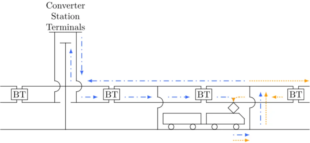
conduction through rail and ground [25]. The complications are primar-ily disturbances on phone and signal systems, caused by ground currents and magnetic fields [81]. The normal distance between BT transformers is around 5 km, and between these, there is a connection between the return conductor and the S-rail, see Figure 2.1. The purpose of the BTs is to draw the current from the return rail to an overhead return conductor. In Sweden one rail is conducting, and is called "S-rail", whereas the other rail is used for signalling and is called "I-rail" [25].

BT BT BT BT

Converter Station Terminals

Figure 2.1: An illustration of a typical BT catenary system. The blue and dash-dotted lines represent current flows corresponding to the converter station behind the train, i.e. to the left in the figure. The yellow and dotted line represent current flows corresponding to the, in the figure not visible, converter station in front of the train.

Through a BT the sum of currents needs to be zero, therefore it will draw the return current from the rail through the return line all the way to the return current bus. The purpose of using the BTs is mainly to reduce the stray currents in the rail [98]. Since the train is moving, the impedances between the locomotives and the nodes of power inflows vary in time. The impedances between the nodes are dependent not only on the physical dis-tances between the them, but also on e.g. the locomotive’s distance to the BTs and return line connectors. Thus, one can say that the impedances vary in a complicated way.

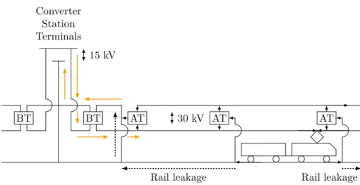
Swedish catenary system [25]. Whereas a BT balances currents, an AT balances voltage. Replacing BT catenaries with AT catenaries doubles the voltage between catenary and the feeder line, but still maintains the same rail-to-catenary voltage as in the BT system. The doubling of voltage is created by a 180 degrees voltage phase shift between the contact wire and the feeder line. This is a way of reducing impedances in a cost-efficient way. The higher voltage leads to smaller currents, and thereby also reduced power losses and reduced telephone interferences [81]. AT transformers are normally distributed with 10 km in between. If the distance to the first AT is more than 2.8 km then a BT is installed in between [25]. If a BT is installed in between the converter stations terminal and an AT system, the wiring and the protection technique in the converter station can remain the same as in the old BT systems. The AT system of Norway works a little bit differently than the Swedish one, [94]. It results in somewhat higher Norwe-gian AT impedances than in the Swedish system, but is a cheaper product. An illustration of one possible installation of the AT catenary technology can be found in Figure 2.2 [44].

30 kV BT BT Converter Station Terminals AT AT AT

Rail leakage Rail leakage 15 kV

Figure 2.2: An illustration of one of many possible AT catenary systems.

The orange and solid arrows in Figure 2.2 show that because of the presence of BT transformers at the feeding points, the return current is the same as the feeding current. In some AT catenary systems there are no BT transformers at all, and in others, the BT transformer is placed very close

to the converter station [44]. The dotted lines represent leakage currents. The leakage current behind the train in Figure 2.2 is related to current originating from the converter station behind the train, i.e. to the left in the figure. Similarly, the leakage current in front of the train in Figure 2.2 originates from the converter station in front of the train, a station that is not visible in the figure. Leakage currents may be harder to handle without BT transformers at the feeding points. In Figure 2.2 the first AT transformer station at the catenary consists of one AT, like a description found in [25]. In fact, it is also quite common to have two AT transformers in the first AT transformer station on the catenary after a converter station [29]. This pair of ATs is normally directly connected to the converter station and it can even be integrated into the converter station [44].

Catenaries above double tracks can either share the same ATs or have one each [81]. In this thesis, such details are not considered.

In AT+BT systems, systems which use a blend of technologies, the AT transformers can be sparser distributed than in a pure AT system. This is possibly a cheaper choice when upgrading old BT systems that have become too weak due to increased traffic. A smaller discussion of AT+BT can be found in [81] where also some further references can be found.

In the literature, different kinds of designations for Swedish catenary standards may be found. Some designations worth mentioning are: "1Å", which means a catenary with a return conductor; "2Å", which means a cate-nary with two return conductors; and "Fö" which means an extra feeding line [43]. Catenaries for double tracks can either be parallel or intercon-nected. The area of the conductors is measured in mm2_{. Interconnected}

catenaries are normally coupled together at stations.

Normally in Sweden the numerical values of the length-dependent AT impedances are four to five times smaller than the corresponding BT impedances. The main reason why the AT length-impedance is smaller than the BT one, besides the doubled voltage between catenary and feeder line, is that the power flows only through two ATs and one BT in each di-rection, irrespective of the distance to the converter station, as can be seen in Figure 2.2. With a BT system on the other hand, the further the train is located from the converter station, the larger is the number of BTs the power has to flow through, see Figure 2.1.

The main drawback with AT is that the ATs do not draw current from the rail in the same was as a BT does [41]. A BT requires the return current to be equal to the ingoing current. Therefore, in AT systems, there

is a somewhat bigger risk for rail and ground currents that could disturb telecommunications and other sensitive equipment. This phenomenon is illustrated in Figure 2.2 with the dotted lines.

Models

A common approximation of BT catenaries [53,81] is a Π-model impedance depending linearly on distance between every pair of nodes. In other words, the BT catenary between a pair of locomotives, a pair of feeding stations, or between a feeding station and a locomotive is modeled with a Π-model. Connection points on the catenary to the HV line , see Section 2.3.2, can, like converter stations, be named feeder stations.

Sometimes AT catenaries are modeled similarly to BTs, but with lower numerical values on the impedances. More commonly [30, 44, 53] the mod-els of the AT lines are divided into a few different impedances: one point impedance in each connection to a feeding point, and one length-dependent Π-model impedance along the railway tracks. The point impedance, or the initial impedance, is illustrated in Figure 2.4 where it is denoted Zinit. A

feeding point is a common name for connections to converter stations or transmission line transformer stations. The length-dependent Π-model for AT is just as in the BT case divided up on n + 1 smaller Π-models if there are n trains between a pair of converter stations.

A justification of the modeling of AT catenaries as length-dependent impedances between the feeders can be found in [118]. The point impedances in the modeling of AT catenaries can at least partly be explained by the fixed number of ATs and BTs that the power has to flow through [41, 43]. This can be compared to BT catenaries, where the current flows through more or less all BTs between the power source and the power sink. The point impedances appear everywhere where a conversion between 15 kV and 30 kV takes place [30].

In the models used in this thesis, it is assumed that between a pair of feeding stations, the catenary runs freely. In other words, the only electrical connection possible to a catenary line between a pair of feeders is a locomo-tive. In reality however, where multiple tracks are present, the catenaries can be connected electrically at every station [81]. Connecting to parallel catenaries at every station increases the capacity to transfer power on the catenary, but would also cause greater problems in cases of e.g. short

cir-cuits. If the parallel catenaries were separated from each other electrically and one of them were short-circuited, then the other one still could be used. The catenary impedance models include catenary impedance, ground impedance, and rail impedance together. In reality, some parts of the return current leave the rail and go back to the converter station through the ground. This can lead to rail-to-ground voltages of up to a few hundred volts. With the modeling proposed here, this voltage level will not be explicitly calculated. For dimensioning purposes, e.g. studies of possible amount of deliverable power to trains, the rail potential can be neglected [37]. In, safety studies on the other hand it might be important to consider the rail potential, e.g. for people walking on the rail [37].

2.3.2 Transmission Line

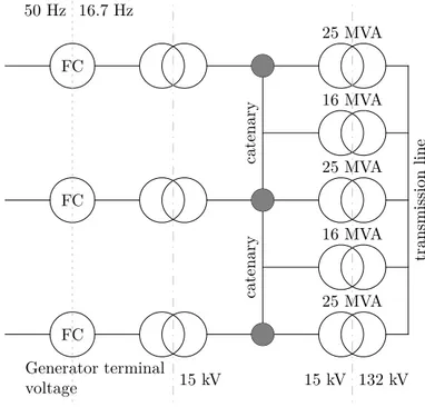
It is common in countries with 16.7 Hz power systems for the railway to have complementary High Voltage (HV) transmission lines, see Figure 2.3. The purpose of these are to:

• reduce the power flows on the catenaries

• relieve pressure from converter stations close to great loads • make the system more redundant

• limit the number of converter stations needed. Each country has its own solution, or solutions.

There are three different voltage levels used in the Swedish two-phase HV transmission lines, 15 kV , 32 kV, and 132 kV [43]. The most common is the 132 kV type. Similar, but not identical solutions can be found in all other European low frequency countries: 110 kV in Germany [79], 55 kV and 110 kV in Austria [58], 66 kV and 132 kV in Switzerland [21], and 55 kV in Norway [88]. In parts of the German railway power supply system where the power flows are large, there are even several HV lines installed in parallel.

Models

At normal operation the two-phase HV line parallel to the railway catenary system is loaded equally on each of the phases. Therefore, the HV lines can

FC FC FC Generator terminal voltage 15 kV 15 kV 132 kV 25 MVA 16 MVA 25 MVA 16 MVA 25 MVA 50 Hz 16.7 Hz ca te na ry ca te na ry tr an sm is si on lin e

Figure 2.3: An illustration of the general idea of transformer usage

easily be approximated as one-phase Π-model impedances depending lin-early on distance. The distances between the catenary and the transmission line are assumed to be negligible. Therefore, the only impedance between the HV line and the catenary that is accounted for is the impedance of the transformer.

2.3.3 The modeled power line impedances in the context of

the power supply system

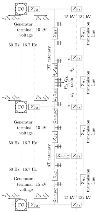
A detailed description of the impedances in the railway power supply system can be found in Figure 2.4. In the figure, there are some denotations that should be introduced.

• The frequency converters are abbreviated FC.

• The impedances on AT and BT catenaries are denoted ZAT and ZBT

• The point-like AT initial impedances are simply denoted Zinit.

• ZT1 and ZT2 both represent transformers.

– The former, ZT1, is the transformer between the catenary and

the HV line.

– The latter, ZT2, is the transformer between the converter station

and the catenary. In the TPSS model this impedance is merged into the Xg

q reactance in the same manner as in [98]. This

mer-gence is described in equation (E.46).

• The length-dependent impedance of the HV transmission line is de-noted ZHV.

• And finally there are the scalars, d1 and d2, describing the by the train

covered fraction of the distance between a pair of feeder stations. Since

d1 and d2 describe fractions of a distance, their sum is one.

Note that, for simplicity, the inter-feeder-station distances in Figure 2.4 are assumed to be homogeneous. In reality, naturally, such distances can vary.

The transformers connecting the HV lines to the low voltage part of the railway power system are modeled as impedances. In Sweden these can be rated for either 16 MVA or 25 MVA, and as can be seen in Figure 2.3 the transformers with the higher ratings are connected to the converter stations. In [81] it is suggested that, due to the risk of transformer outages, two 16 MVA transformers should be installed at the converter stations instead of one 25 MVA transformer.

2.4

The Frequency Converters

2.4.1 Background

Since the public power grid is 50 Hz and it is attractive to be able to transmit electrical power between the public and the railway power grids, frequency converters are needed. Nowadays in Sweden, there is no 16.7 Hz power production at all, so the need for converters is even stronger here.

There are two main types of frequency converters, rotary and static. Ro-tary converters consist of one motor and one generator attached to the same shaft. Static converters are built using power components. In the Swedish

ZT2 FC ZT2 FC ZT2 FC −PG, Q50 −PG, Q50 −PG, Q50 PG, QG PG, QG PG, QG Generator terminal voltage 15 kV Generator terminal voltage 15 kV Generator terminal voltage 15 kV 50 Hz 16.7 Hz 50 Hz 16.7 Hz 50 Hz 16.7 Hz Zinit,T Zin it ,F C Zin it ,F C ZT1 ZT1 ZT1 ZT1 ZT1 15 kV 132 kV 15 kV 132 kV d1 ZB T d2 ZB T PD ,Q D tr ai n d1 d2 ZB T B T ca te na ry ZA T ZA T A T ca te na ry ZH V tr an sm is si on lin e ZH V tr an sm is si on lin e ZH V tr an sm is si on lin e ZH V tr an sm is si on lin e

16.7 Hz railway power system, according to regulations, static converters do not have to be able to send back regenerated electric power to the 50 Hz grid, but if they can do it they must have the ability to turn that func-tion off [80]. Rotary converters can always send power in both direcfunc-tions by their construction. Regenerated power is produced by locomotives with regenerative brakes that convert kinetic energy to electrical while braking. All converters must be able to manage regenerating locomotives without, e.g. tripping.

Realistic distances between a pair of converter stations can vary from 40 up to 160 km [47], and there can be between two and five converters in each station. Of course, for a given level of train traffic, the converters can be more sparsely distributed, within the range 40 to 160 km, if the catenary is connected to an HV line than if it is not.

Converter losses are never zero, and moreover, they tend to increase relative to the power throughput the lower the load [88]. Therefore, the converters are connected and disconnected with a so-called "start and stop automation". This means, that if the converters in a converter station are loaded below a predefined threshold, one of them is disconnected. Con-versely, if the converters in a converter station are loaded above a different predefined threshold a nearby converter is connected. This automation is not currently included in the TPSS simulator model of Chapter 3, but is included in TracFeed Simulation [38].

The active power flow through a frequency converter station is deter-mined by machine parameters and the voltage phase angle difference be-tween the 50 Hz and the 16.7 Hz sides of the converter station. To be exact, this is only true for stations consisting of rotary converters, because static frequency converters can among other things control their amounts of con-verted power freely.

In a Master’s thesis, it has been shown that one can, at a relatively low cost, also control the phase angles, θ50_{, on the 50 Hz sides of the rotary}

converters [77]. The suggested method of controlling the angles is to connect inductors and capacitors between the 50 Hz grid and the 50 Hz side of the converter station. Since this connection and disconnection of capacitors and inductors controls the phase angle on the 50 Hz side of a rotary converter, it also controls the phase angle difference between the 50 Hz and the 16.7 Hz sides of it. Thus, one can with this 50 Hz side voltage phase angle control, also control the power flows through the rotary converters.

which is the case in Sweden. The fact that static converters mimic rotary converters allows a modeling of static converters that is quite similar to the modeling of the rotary converters [97,98]. The main exception is that static converters cannot be overloaded, limiting the active power flows through them [80]. When the active power flow through a static converter is at its maximum, the converter starts to have different voltage angle characteristics than rotary converters have [80].

Power losses in locomotives and power converters are not considered in this thesis. Power losses in converters are modeled in [81, 98], and can be implemented in TPSS later on if considered of interest.

2.4.2 Models

Based upon the discussion in Section 2.4.1, no difference is made in the models if a converter is static or rotary in this thesis. All converters of the same size are modeled the same.

Not even a rotary converter can be too heavily overloaded for a long time. This issue is however not formulated as a constraint in the TPSS models used and presented in this thesis, but can be checked afterwards, by postprocessing TPSS results. The exact limitations of rotary converters loadings are e.g. listed in [73, 98], where the latter contains more details.

In [97,98] one can find more general models for different compositions of converter stations, i.e. for different types and different numbers of converters connected in parallel inside the station. In the TPSS models presented in this thesis however, only converter stations consisting of converters of the same kind are considered. In converter stations with only converters of the same kind, the total amount of active power injected on the 16.7 Hz side,

PG, the total amount of reactive power injected on the 16.7 Hz side, QG,

and the total amount of reactive power absorbed on the 50 Hz side, Q50,

can simply be equally divided by the number of converters, #conv, in order

to give the proper catenary voltage, U, and the phase angle difference, ψ, values [98]. This division can be seen in equations (2.1) and (2.3).

The model used for the rotary converters originates from [80, 97, 99]. In [97,99] it is assumed that the generator side voltage of the frequency con-verter, Ug_{, is controlled at 16.5 kV. In reality however, a kind of terminal}

voltage control called "amplitude compounding" is used. This terminal volt-age control is described by equation (2.1). This description of "amplitude compounding" comes from [80] and is used also in the models of TPSS of

this thesis. In equation (2.1), Ug _{is expressed in kV, Q}

Gin MVAr, and #conv

is an integer, i.e. the number of converters used in the particular converter station.

The commercial simulator TracFeed Simulation uses dynamic models for the converters, so the models for the terminal voltage control are far more advanced than the steady state models presented in this thesis. In TracFeed Simulation/Simpow, the feedback signal for the voltage control depends on voltages, currents, and reactive compensations [110].

The relations between 16.7 Hz side power generation and the system voltages/angles can be concluded in the following four equations

Ug _{= 16.5 −} QG #conv· 20 (2.1) θ0 = θ50 − 1_{3 ·}arctan X50· PG (Um₎2_{+ X} 50· Q50 (2.2) ψ = −1₃arctan X m q ·#PconvG (Um₎2_{+ X}m q · Q50 #conv − arctan X g q ·#PconvG (Ug₎2_{+ Xq}g_· QG #conv (2.3) θ = θ0+ ψ (PG, QG, U ) (2.4)

where Q50 denotes the reactive power absorbed on the 50 Hz grid side,

i.e. the motor side of the converter, X50 is the short circuit reactance of the

50 Hz system, i.e. the reactance between the motor side of the converter station and the strong grid [98], θ50_{is the no-load phase angle on the 50 Hz}

side, Xm

q and Xqg are quadrature reactances of motor and generator

respec-tively, Um_{and U}g_{are the motor and generator side voltages, P}

Gand QGare

the generated active and reactive powers at the generator side. The 50 Hz grid is assumed to be sufficiently strong for the assumption that Um _always

is at a nominal level. The voltage phase angle on the 50 Hz side of the converter taking the train power consumption into account, θ0_{, is described}

by equation (2.2) [98] and defined with opposite sign and direction of Q50

in [99]. Finally, ψ is the phase angle difference between the 50 Hz and the 16.7 Hz sides of the converter.

The models presented in this section are purely static. When using dy-namic models of the frequency converters, the models immediately become more intricate. The commercial simulation software TracFeed Simulation uses the dynamic converter models [110] (chapters 21-25) of Simpow [111].

2.5

Locomotives and Trains

2.5.1 Introduction

In this section of the thesis, the focus is on the in Sweden most common loco-motives, the Rc-locomotives. Another reason to study the Rc trains, besides their major usage, is their peculiar reactive power consumption properties. The locomotives used in Sweden before the Rc locomotives came, had a discrete set of tractive power levels to choose from. In order to allow the locomotive engineer a continuous power control, using the technology of the time when the Rcs were constructed, there was a need to compromise with the power factor [41]. Thus, the locomotives before the Rcs did not consume as much reactive power as Rcs do, but on the other hand, could their tractive forces not be smoothly controlled. Rc locomotives were produced between 1967 and 1988 [74]. Rc locomotives are today mostly used for hauling goods transports and for long-distance personal transports, e.g. night trains, but can still be used for some short-distance passenger trains as well. Pre-Rc locomotives are hardly not used at all.

It might be worth noting that there are a variety of Rc locomotive types. The Rc-locomotive models presented here are close to a so called ”Rc4” lo-comotive, but most of the assumptions would be similar for other Rc de-signs [74]. In principle, Rc4 are used for goods trains, and Rc6 for passenger trains. Most of the remaining Rc locomotive types have been phased out or rebuilt [74]. Rc locomotives can, depending on which type it is, have intended maximal speeds of either 135, 160 or 180 km/h [74]. In this thesis, the focus has been set on goods trains, thus the 135 km/h limit is used here. Locomotives and rail motor coaches produced in Sweden after the Rc era, have three-phase asynchronous engines where both active power and reactive power can be controlled. The active power inflow/outflow is of course the same on both sides of the on-train converter, if neglecting converter losses. The reactive power, on the other hand, is not the same on both sides. What is consumed by the locomotive, i.e. the reactive power produced on the motor side of the on-train converter, is in general not the same as the reactive power consumed on the caternary/pantograph side of the on-train converter. How much reactive power that in fact is consumed by the locomotive engine is of secondary interest from the power system dimensioning point of view. What is interesting though, is how much reactive power that flows from the catenary to the on-train converter. That is why reactive power is controlled

on the catenary/pantograph side of the on-train converter.

Rail motor coaches are used for local or regional passenger transports. Their advantages compared to locomotive driven ones are that there is room for more people per cubic meter, and that they have better acceleration. Locomotive driven passenger trains are usually used for faster, more distant transports, with not so many intermediate stops. The most common such train in Sweden is X2, brand named X2000 by the national operator SJ AB. The strongest MTAB (MalmTrafik i Kiruna AB) locomotives can consume up to 12 MW [25].

Auxiliary power needs in the trains, e.g. heating, cooling, lights, venti-lation, and laptop power, is not included in the TPSS models. There exists a lot of models for this, so it might be included in the future.

2.5.2 Common Models for Tractive Force and Tractive

Power Limits and Regulation

The maximal tractive force of most locomotives, including Rcs, is a function of the catenary voltage, U, and the velocity of the train, v. The function can be expressed in different ways. The tractive force limit with respect to voltage and velocity is a physical limitation, related to the internal currents of the locomotive. Some similar additional limits regarding tractive force, consumed locomotive power, and the train acceleration are sometimes also present, but these are man-made, and suits therefore better to be called controls.

First the physical limitation will be presented in a section. After that, in the next section, some examples of common controls will be listed and one of them will be described in some more detail.

Common Tractive Force Models

The maximal tractive force, Fmotor,max, as a function of catenary voltage, U,

and train velocity, v, is, as mentioned in the preceding paragraph, a physical limitation of the locomotive. This tractive force upper limit is normally modeled as a piecewise continuously differentiable continuous function with respect to velocity as well as to voltage level. That particular model of

Fmotor,max, which is described in the following text, is the easiest one to draw

by hand and an example of it can be found illustrated in Figure 2.5. This easily-drawn model is used in the train traffic and power supply simulation

0 100 200 0 100 200 300 v (km/h) F (k N )

(a) The maximal tractive force is here, first, the smallest of the curves where, F_{, F · v, and F · v}2

are constant, re-spectively. Then, from the velocity of 160 km/h and on, the maximal tractive force abruptly equals zero.

0 100 200 0 100 200 300 v (km/h) F (k N )

(b) The maximal tractive force, plotted for different catenary voltage levels. The blue curve represents a catenary voltage of 16.5 kV, whereas the green curve rep-resents 15 kV, the red curve 13.5 kV, the cyan curve 12 kV, and finally, the ma-genta one 10.5 kV.

Figure 2.5: A description of a typical maximal tractive force curve for an electric locomotive. This figure is inspired by the particular modeling used in TracFeed Simulation.

program TracFeed Simulation [109]. A similar model, but without the part where F · v2 _{is constant is presented in the paper [63] as well as in the}

Master’s thesis report [75], whereas it is applied in the successor [76]. The maximal tractive force, Fmotor,max, is first constant, 275 kN in the

illustrated example of Figure 2.5, from standstill up to a certain breaking velocity, 78 km/h in the example of Figure 2.5a. Thereafter the maximal tractive force starts to decrease with 1

v, i.e. F · v is kept constant. In the

third step, F · v2 _{is kept constant between the part where F is proportional}

to 1

v and the part where the tractive force equals zero. The exact behavior of

the locomotive for extreme velocities is normally not interesting, therefore the tractive force is commonly modeled to abruptly go down to zero when the velocity is too high.

The voltage dependency is in the model of TracFeed Simulation modeled as if F is related proportional to U

Unom when the catenary voltage, U, is less than Unom, the nominal voltage [108]. This voltage dependency is valid only

be seen in Figure 2.5b. In the example of Figure 2.5b, the nominal voltage is defined to be 16.5 kV, though it normally is defined to be 15 kV. For catenary voltages above Unom, the tractive force is not changed [108].

The effective tractive force can also, in some more detailed models, be depending on a velocity dependent efficiency factor [109].

Common Controls on Tractive Force, Tractive Power, and Train Acceleration 10 12 14 16 18 0 2 4 6 8 U (kV) P (M W )

(a) Example of active power control

10 12 14 16 18 −5 0 5 U (kV) P ow er an gl e (d eg re es )

(b) Example of power angle control

Figure 2.6: Examples of active power control and power angle control on lo-comotives. The dashed curve represents a motoring locomotive, whereas the dotted curve represents a locomotive using regenerative braking. Inspiration is taken from a figure found in [113]

Controls limiting the locomotive’s tractive force, tractive power, and the acceleration of the train can be designed in many ways. Some of the more common are

1. tractive electric power and the power angle with respect to catenary voltage

2. tractive force with respect to catenary voltage alone, i.e. independent of velocity

3. tractive force with respect to velocity alone, i.e. independent of cate-nary voltage

4. acceleration and deceleration with respect to velocity.

The purpose of point 1 in the list above is to reduce the risk of overloading the power system. An example of active power control can be found in Figure 2.6a for both motoring and braking of the train. Normally, at least in Sweden, such additional controls are in use [38]. That results in a higher sensitivity of train delays caused by voltage drops than presented in the results of this thesis.

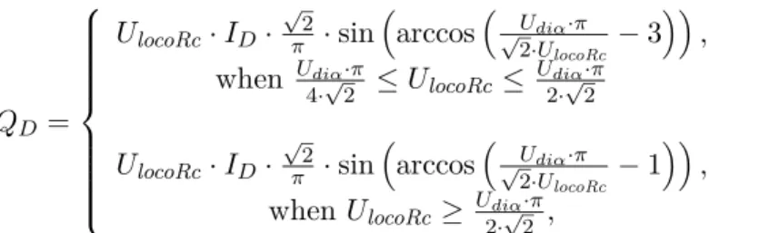
The power angle can be controlled only on locomotives or rail motor coaches with three-phase asynchronous motors, where the consumed reactive power, QD, can be controlled freely within some limits. However, such

operation could cause compatibility problems with the existing protection system [30]. Other risks could be instability in the system and difficulties for several nearby trains to regenerate at the same time [30]. Therefore, the three-phase asynchronous locomotives of today in operation in Sweden are purely resistive, i.e. letting QD equal zero, no matter if consuming or

regenerating power.

It is however tempting to let the locomotives behave capacitively, when driving for voltages below nominal, and resistive for voltages above the nom-inal level. Furthermore, when braking regeneratively it might be desirable to let the locomotives behave as reactors when the catenary voltage is under nominal and as capacitors when the voltage is above nominal. If this is done, it is done with the intention of keeping the catenary voltage level as close to nominal as possible. Here, a capacitive behavior of a locomotive means that if it consumes active power it produces reactive power – and conversely if it brakes regeneratively it consumes reactive power. Consequently, a reactive behavior must mean the opposite. A motoring locomotive consumes reactive power whereas a regenerative one produces reactive power.

The above described locomotive behavior is, in order to further clarify, also described by a picture, instead of just by words, as can be seen in the example of Figure 2.6b. In that figure, QD shifts sign at 135·2₁₇ kV which is

about 15.88 kV when regenerating, and it becomes zero when the catenary voltage goes above 16 kV and the train is motoring.

Point 4 in the above numbered list is mainly explained by a desire to minimize the occurrence of quick and uncomfortable changes in the train velocity.

2.5.3 The Electrical and Mechanical Power Consumption Models used in this Thesis

The new models of this thesis are developed with the intention to be used in the Matlab & GAMS simulator package called TPSS (Train Power Sys-tem Simulator) presented in Chapter 3. Since GAMS prefers equations that contain continuous variables to discrete variables, and equations hav-ing continuous derivatives to functions not havhav-ing that; such as: max, min, and absolute value; and since the tractive force curves available were in the format they were, the models of maximal tractive forces used in this thesis are nonlinear backpropagation [59,62] Neural Networks (NN). The maximal tractive force curves available are scanned from an old paper manual, found in an appendix to [74], see Figure 2.7 for examples. The NNs are used for finding mathematical expressions of relations between inputs and outputs, i.e. they are function estimators.

Here, the inputs are velocity and voltage, whereas the output is the max-imal tractive force. Both training input and training output are normalized to lie within the span [−1, 1] before training. The number of hidden neu-rons depends on what seems to suit best for the respective characteristic curves. Quite arbitrarily, the number of hidden layers were limited to just one such. Also the choices of tanh, or tansig if using NN terminology, as transfer functions were made arbitrarily. The output layer has linear trans-fer functions, and the algorithm used for NN training is the in-built Bayesian regularization training algorithm, trainbr [6], of Matlab’s NN toolbox.

When approximating the Rc locomotive curves of [74] with the maximal short-time tractive force, i.e. the one that results in an internal locomotive-current of 2080 A, see Figure 2.7 for examples, good approximations are obtained when using 15 neurons in the hidden neuron layer. Numerical values of the NN coefficients can be found in the appendix Section B.1.

For the maximal continuous tractive force, i.e. the CONT curve in the example graphs of Figure 2.7, 6 neurons in the hidden layer gives the best approximation. Numerical values of the NN coefficients can be found in the appendix Section B.2.

The approximation of the maximal short-time curve can be found plot-ted in Figure 2.8a, whereas the approximation of the continuous curve is to be found in Figure 2.8b. The reader should note that the old curves in Figure 2.7 are expressed in Mp (Mega pond), whereas the approximations in Figure 2.8 are expressed in kN, the standard of today. The *s in Figure 2.8

represent points measured in the [74] graphs as well as some points forcing the curves down to zero for high velocities. Apart from Figure 2.7a and Figure 2.7b, there are three more graphs in the document [74]. The docu-ment contains altogether five graphs, one for each of the catenary voltage levels 10.5 kV, 12 kV, 13.5 kV, 15 kV, and 16.5 kV. Three points are used, for each of the five measured voltage levels, for forcing the curves down when the velocity is high. These fifteen extra points were together with the measurements used for neural network training.

The observant reader notices that the NN generalizes in a reasonable manner also for the unmeasured 9 kV and 18 kV catenary voltage levels. The tractive force curves of some of the Rc locomotives in use today are somewhat modified compared to, e.g. Figure 2.7, [33].

(a) For catenary voltage 10.5 kV (b) For catenary voltage 16.5 kV

Figure 2.7: Original diagram describing the maximal tractive force as a function of velocity for different motor currents, source [74]