2009:16 Influence of Hardening Model on Weld Residual Stress Distribution

Infl uence of Hardening Model on

Weld Residual Stress Distribution

Research

Authors:

2009:16

Title: Influence of Hardening Model on Weld Residual Stress Distribution. Report number: 2009:16

Authors: Jonathan Mullins and Jens Gunnars Inspecta Technology AB, Stockholm, Sweden Date: June 2009

This report concerns a study which has been conducted for the Swedish Radiation Safety Authority, SSM. The conclusions and viewpoints pre-sented in the report are those of the author/authors and do not neces-sarily coincide with those of the SSM.

Background

Weld residual stresses have a large influence on the behavior of cracks growing under normal operation loads and on the leakage-flow from a through-wall crack. Accurate prediction of these events is important in order to arrive at proper conclusions when assessing detected flaws, for inspection planning and for assessment of leak-before-break margins. Therefore, it is very important to have verified procedures to estimate weld residual stresses (WRS). During the latest years, there has been a strong development in both analytical procedures to numerically determine WRS and experimental measurements of WRS. The present report is the result of an effort to acquire and to develop the latest research results in the field of WRS and especially the influence of hardening model. The choice of hardening model has been the subject of intense studies lately among research groups around the world for simulating weld residual stresses.

Objectives of the project

The principal objective of the project is to use the latest research results of determining WRS in piping components, especially the choice of hardening model and verify such procedures against experimental measurements.

Results

Welding simulations were conducted using isotropic, kinematic and mixed hardening models. The isotropic hardening model gave the best overall agreement with experimental measurements; it is therefore re-commended for use in welding simulations. The mixed hardening model gave good agreement for predictions of the hoop stress but tended to under predict the magnitude of the axial stress. The kinematic harde-ning model consistently under predicted the magnitude of both the axial and hoop stress and is not recommended for use.

Effects on SSM

The results of this project will be used by SSM in safety assessments of welded components with cracks.

Project information

Project leader at SSM: Björn Brickstad

Project number: 14.42-200542009, SSM 2008/77

Project Organisation: Inspecta Technology AB has managed the project with Dr Jens Gunnars as the project manager.

Contents

1 SUMMARY...2

2 INTRODUCTION...3

3 RESIDUAL STRESS MODELLING PROCEDURE ...5

3.1 Transient thermal analysis ...5

3.2 Thermo-elastic-plastic mechanical analysis ...7

4 MATERIAL PROPERTIES AND HARDENING MODELS ...9

4.1 Thermal properties and the coefficient of thermal expansion...9

4.2 Sources of data for plastic deformation of 316 stainless steel ...9

4.3 Models for material hardening...10

4.3.1 Isotropic ...10

4.3.2 Kinematic ...12

4.3.3 Mixed isotropic and kinematic...13

4.3.4 Perfectly plastic (non strain hardening)...14

4.3.5 Viscoplastic...14

5 SIMULATIONS AND VALIDATION TO MEASURED RESULTS ...15

5.1 Case 1 – Intermediate pipe ...16

5.2 Case 2 – Thick-walled pipe ...22

5.3 Comments on the choice of hardening model...27

6 SENSITIVITY ANALYSES ...29

6.1 Use of bilinear hardening where there is a small saturation strain ...29

6.2 Effect of introducing viscoplasticity...30

7 DISCUSSION AND RECOMMENDATIONS FOR FUTURE WORK ...32

7.1 Recommendations for future work ...33

8 CONCLUSIONS...35

9 REFERENCES...36

1

SUMMARY

This study is the third stage of a project sponsored by the Swedish Radiation Safety Authority (SSM) to improve the weld residual stress modelling procedures currently used in Sweden. The aim of this study was to determine which material hardening model gave the best agreement with experimentally measured weld residual stress distributions. Two girth weld geometries were considered: 19mm and 65mm thick girth welds with Rin/t ratios of 10.5 and 2.8, respectively. The FE solver ABAQUS

Standard v6.5 was used for analysis.

As a preliminary step some improvements were made to the welding simulation procedure used in part one of the project. First, monotonic stress strain curves and a mixed isotropic/kinematic hardening model were sourced from the literature for 316 stainless steel. Second, more detailed information was obtained regarding the geometry and welding sequence for the Case 1 weld (compared with phase 1 of this project).

Following the preliminary step, welding simulations were conducted using isotropic, kinematic and mixed hardening models. The isotropic hardening model gave the best overall agreement with experimental measurements; it is therefore recommended for future use in welding simulations. The mixed hardening model gave good agreement for predictions of the hoop stress but tended to under estimate the magnitude of the axial stress. It must be noted that two different sources of data were used for the isotropic and mixed models in this study and this may have contributed to the discrepancy in predictions. When defining a mixed hardening model it is difficult to delineate the relative

contributions of isotropic and kinematic hardening and for the model used it may be that a greater isotropic hardening component should have been specified. The kinematic hardening model

consistently underestimated the magnitude of both the axial and hoop stress and is not recommended for use.

Two sensitivity studies were also conducted. In the first the effect of using a bilinear model with a saturation strain of 0.01 was evaluated. This model was not capable of accurately predicting the weld residual stress field and its use is not recommended.

In the second sensitivity study, the effect of defining a viscoplastic model was evaluated. For predictions of axial and hoop stress, the viscoplastic model was found to give slightly lower stress peaks, although the effect was sufficiently small that the increased complexity and computational cost of defining such a model probably outweighs the benefits. It was noted that a similar effect could be obtained by lowering the annealing temperature.

2

INTRODUCTION

Detailed knowledge of the residual stress fields that result from welding processes is critical to performing damage tolerance analyses of nuclear structures. The through-thickness distribution of these weld residual stress fields influences the growth of cracks where either stress corrosion cracking or fatigue is of interest. This distribution is sensitive to geometry, material and welding parameters and must be accurately predicted in order to reach safe conclusions about structural integrity. For this reason considerable effort has been devoted to quantifying weld residual stress fields both

experimentally and numerically. This study is the third part of a project sponsored by the Swedish Radiation Safety Authority (SSM) to improve the weld residual stress modelling procedures currently used in Sweden. The focus of this study is on material hardening models.

In the past, welding simulation has been conducted using a kinematic hardening model but with recent developments in the area there has been a shift to the use of isotropic and even mixed hardening models. From the literature it is unclear which hardening model is best or even whether there is a significant difference in the residual stress fields obtained. In the first part of this project [1] an isotropic model provided a better agreement to experimental data for a range of girth weld geometries as compared to a kinematic model. Conversely, Ogawa et al [2] recently published results which indicated that the choice of hardening model did not have a significant influence on the weld residual stress field. Ogawa’s results are, however, difficult to interpret because full details were not available regarding how the isotropic, kinematic and mixed hardening models were defined.

It is important to note that the definitions ‘isotropic’, ‘kinematic’ and ‘mixed’ do not fully define hardening characteristics of a material. There are many ways in which each of these types of hardening can be specified and these details, which are typically not reported in the literature, can drastically affect the shape of a weld residual stress distribution.

In this work we attempt to identify the effect that different hardening definitions can have on weld residual stress distributions and therefore rationalise the two apparently contradictory findings cited above. Further, a recommendation will be made regarding which hardening model is most appropriate for future use in weld residual stress simulations. As a first step, it is proposed that a review should be conducted of available material data and best estimate properties for 316 stainless steel be obtained. It is then proposed to compare the weld residual stress fields produced by the different hardening models with experimentally measured data. In the main part of this study three different hardening models are considered, for two girth weld geometries:

 Isotropic, where flow curves at different temperatures are fully defined in tabular form.  Kinematic where the Ziegler implementation is used.

 Mixed isotropic and kinematic (Lemaitre-Chaboche, 1990) [3] hardening with fully defined, nonlinear isotropic and kinematic hardening definitions.

Two sensitivity studies are also conducted in which a single girth weld geometry is considered but where additional material hardening behaviours are considered.

The first sensitivity study considers a special implementation of the isotropic and kinematic hardening models where hardening is only allowed up to a small saturation strain of 0.01. Beyond the saturation strain no further strain hardening occurs. This sensitivity study is proposed as a possible explanation of the results reported by Ogawa [2], as discussed above and also because hardening models such as

these have been used for weld residual stress simulation in the past [4]. To test this hypothesis, the following hardening models are considered:

 Perfectly plastic (no strain hardening) as a reference material model.  Bilinear isotropic hardening where the saturation strain is 0.01.  Kinematic (Ziegler) hardening.

A second sensitivity study is proposed to quantify whether strain rate effects significantly influence the shape of the weld residual stress field. It is possible that a viscoplastic model will allow some stress relaxation during bead cooling. Further, a viscoplastic model may more accurately capture the deformation process during the addition of a weld bead where there is a high thermal gradient and therefore a relatively high rate of deformation. For this sensitivity study the following material hardening models are used:

 Isotropic, where flow curves at different temperatures are fully defined in tabular form.  Viscoplastic where tabulated isotropic hardening is defined together with a strain rate

sensitivity.

Each of the hardening models listed above is also temperature dependent. Parameter values are defined at a range of different temperatures and flow stresses are interpolated for the temperature of interest.

3

RESIDUAL STRESS MODELLING PROCEDURE

The procedure used in this work is the same as that developed in the first stage of this project [1].

3.1 Transient thermal analysis

The weld residual stress modelling procedure starts with a transient thermal analysis of the welding heat flow. Addition of new molten weld material is modelled using the element-include technique (inactive elements). If necessary, quiet element technique (a low stiffness deforming mesh) could be used in order to achieve a good deformation and adaptation of the element mesh for the non-added beads. The transient thermal history provides input for a subsequent incremental thermo-plastic analysis. Similar to the earlier procedure, the thermal material properties used are temperature-dependent. A heat transfer boundary condition is applied at all free surfaces of the component. The free boundary is altered in space as new weld passes are added. The boundary condition is described by a resulting heat transfer coefficient h (approximating both convection and radiation), given by [5]:









The heat source model for a specific welding method needs to be calibrated by different methods, as use of theoretical models and experimental data. From etched cross sections of a weld by the actual welding process and in the actual material, metallurgical information can help to identify what temperatures there have been at different distances from the melted material in the weld pool. Cross sections also give information on the typical shape of the weld pool and the sectional area of the bead fusion zone resulting from the welding process used and different sets of weld parameters. Information for the heat source modelling can also be provided from temperature measurements very close to weld passes by thermal gages, and by thermal imaging methods for assessing the length of the weld pool. The weld pass heat input per unit run length Q can be calculated from welding process parameters as

(3.2)

where I is the current, U is voltage,  is the electrical heat input efficiency per welding process, and v

is weld travel speed. The heat input efficiency for different welding processes is typically 0.95 for SAW, 0.8 for MMA (or SMAW), and 0.6 for TIG.

When a 2D approximation is used, e.g. rotational symmetry for simulating pipe girth welding, the assumed conditions in the model resemble those corresponding to a simultaneous deposition of the weld pass along the entire weld length. The heat conduction in the welding travel direction is by definition ignored in a 2D model, and the heat input to the structure is exaggerated. This implies an extra need for calibration of the heat source model in 2D models in order to avoid overheating from the simulation.

v IU Q

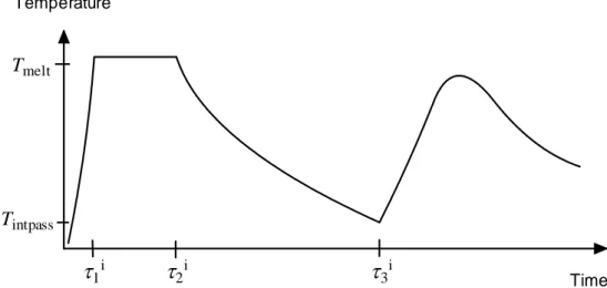
A typical heat source model for arc welding process as MMA, SAW and TIG is illustrated by Figure 3.1. The figure shows the temperature in the centre of a newly added weld bead. The temperature is rapidly rising to the melting temperature Tmelt and the filler material holds that

temperature under the period 2i -1i, before it starts to cool down and solidify, since the weld pool is

moving on. For these welding processes the dominating part of the melted material is new added filler material, and the majority of Q is consumed in the new filler material. The time 1i is short compared

to 2i. The material continues to cool down and has the temperature Tintpass at the instant 3i when the

next adjacent weld pass is made. The temperature Tintpass is the inter-pass temperature, and is often

about 150 °C. The time 3i is long compared to 2i.

Temperature

Time

T_melt







T_intpass

Figure 3.1. Temperature transient in newly deposited weld pass a function of time.

The steps in the transient heat condition analysis of a weld are described below. A two-dimensional model is considered, and a description of a procedure for the heat source calibration for a 2D axi-symmetric model is included. Any specified pre-heating is modelled by a corresponding initial

temperature step for the pipe. The thermal modelling of a new weld pass involves the following steps: 1) A new weld pass to be deposited receives a temperature slightly higher than the melting

temperature Tmelt. The addition of molten weld material is modelled using the element-include

technique, i.e. a group of elements representing the new weld bead is activated. The size of the fusion zone/bead is related to the weld bead cross sectional area achieved from metallographic macro cross sections of the weld for the actual set of welding parameters.

2) A transient heat conduction analysis is then performed to simulate the subsequent heat transfer process after the new weld bead is introduced. The weld bead has the temperature Tmelt under

- The heat affected zone (HAZ) size is determined by the 3D analytical solution for a

given pipe thickness, the thermal diffusivity of the material, and the linear heat input Q and the travelling speed v for the actual weld pass.

- The HAZ size is defined by the distance between the fusion line and nearest position

that reaches to the first phase transformation.

- For the 2D model, the next step is to calibrate the time 2i by analytical solution, in

order to compensate for the missing heat loss in the welding direction (the hoop direction), compared to a 3D travelling heat source.

3) The inter-pass time 3i is adjusted to receive the prescribed overall inter-pass temperature Tintpass

before the next weld pass is activated.

4) The procedure is repeated until all weld beads are added, and then the entire model reaches steady-state room temperature conditions.

5) Any post-weld heat treatment is modelled, and any other thermal loading that may redistribute the residual stress field is modelled.

3.2 Thermo-elastic-plastic mechanical analysis

Once the temperature history is generated using the procedure described above, stresses and strains are calculated by performing a thermo-elastic-plastic analysis. The analysis follows the given temperature history on a pass per pass basis, until all weld passes are simulated.

The mechanical properties are temperature-dependent. Incremental plasticity is used with the

von Mises yield criterion and associated flow rule. Parent and weld material were assigned the same material properties. Details regarding the material hardening laws used are found in Section 4. The multi-pass weld is modelled by activating the elements belonging to the current pass at a proper time, consistent with the transient heat flow simulation procedure. Strain relaxation for material that remelts is simulated using the new annealing capability in ABAQUS.

Few experimental results are reported about the exact extent of which weld strains are annealed, or the extent of strain relaxation in re-heated or re-melted material. Local stress-strain curves in as-welded material are presented in [12] and [24] and the measured local yield stress in as-welded filler material and in HAZ corresponds to 5 - 10% strain hardening of the base/virgin material. This could indicate some degree of strain relaxation, since simulations often generate more strain than that.

Annealing and strain relaxation arises at high temperatures, due to different microstructural processes as recrystallization and rapid creep. Conventional annealing is performed using long hold times (hours) and starts with temperatures from 1/3 of the melting temperature. However, for the rapid temperature transient during welding the amount of annealing in different regions, and the dominating process, is not clarified. It is expected that annealing effects are only seen in regions of much higher temperatures than 1/3 of the melting temperature, because of the short effective hold time.

By utilizing the anneal temperature capability in ABAQUS it is possible to prescribe a temperature above which strain-free conditions are assumed, in order to reset accumulated plastic strains and the hardening. The anneal temperature can simulate rapid strain relaxation at high temperatures, or in re-melted material. Data for the rate of recrystallization or creep at high temperatures is however rare, but

recently published data [19] promotes an argument for a high anneal temperature – greater than 1300ºC.

Boundary conditions resembling the fixing conditions used (and possibly altered) during the welding are applied to the model. Any post-weld heat treatment and other mechanical loading that may redistribute the residual stress field is modelled.

4

MATERIAL PROPERTIES AND HARDENING MODELS

The thermal properties and the coefficient of thermal expansion for 316 stainless steel are displayed in Table 4.1.

Table 4.1 Thermal properties for stainless steel (316) [14].

Temperature [oC] Conductivity [W/m/oC] Specific heat [J/kg/oC] Thermal expansion [10-6/oC] 20 14.7 450 16.4 100 15.8 487 16.8 200 17.2 520 17.2 300 18.6 537 17.9 400 20.0 548 18.5 500 21.1 555 18.6 600 22.2 562 18.7 800 25.2 587 19.1 1000 28.1 611 19.3 1200 30.9 635 19.8 1300 32.4 647 20.0 1390 33.8 659 ~

4.2 Sources of data for plastic deformation of 316 stainless steel

As discussed earlier, welding processes involve plastic deformations over temperatures ranging between room temperature (20ºC) and the melting point (approximately 1400ºC for 316 stainless steel). It is therefore important to use an accurate description of the material properties over this temperature range. A traditional source of material data for 316 stainless steel is the standard ASME 240 [15] but for welding simulation these minimum specified mechanical properties are not

recommended, since they will lead to an underestimate of the magnitude of weld residual stresses. Instead other, best estimate, sources of data are needed. For isotropic and kinematic hardening models, the yield stress and the strain hardening properties must be specified up to, and exceeding a true plastic strain of approximately 0.15. For mixed kinematic hardening models cyclic stress strain curves are required for relevant strain ranges.

A number of sources of mechanical data for 316 stainless steel were identified:

1. In part 1 [1] of the current project Inspecta Technology used mechanical properties obtained during the NESCIII project [16].

2. Sandmeyer steel company [17] specified the yield stress and ultimate tensile stress of 316 stainless steel for temperatures ranging between 20 and 871ºC.

3. Albertini et al [18] published flow curves for 316H stainless steel at strain rates between 10-3 and 10 s-1 for temperatures of 20, 400 and 550ºC.

4. Lindgren et al [19] published flow curves for 316L stainless steel at strain rates between 5x10-3 and 10s-1 for temperatures between 20 and 1300ºC.

5. Van Eeten [20] published cyclic stress strain data for 316L stainless steel for a range of strain ranges at room temperature.

6. Ohmi et al [21], [22] published cyclic stress strain curves for 316 stainless steel for temperatures ranging between 20 and 700ºC.

7. Leggatt et al [23] published parameters for a mixed hardening model for both 316L and 316H stainless steel for temperatures between 20 and 1400ºC.

There was no single source that could be used to fully define all the models in this study. Instead two data sources were chosen. Data for the isotropic and kinematic hardening models in this study were taken from Lindgren et al [19] since the yield stress, monotonic strain hardening response and strain rate sensitivity were fully defined for the temperature range of interest. This is both the most recently published and most complete source of monotonic stress-strain curves for 316 stainless steel

commonly available in the literature.

Data for the mixed hardening model was taken from Leggatt et al [23] since a full set of mixed hardening parameters was available for the temperature range of interest.

4.3 Models for material hardening

4.3.1 Isotropic

With isotropic hardening the yield surface expands with accumulated plastic strain. In the implementation used here plastic incompressibility, initial isotropy, isotropic hardening and the normality rule are defined. Yielding occurs when

0     _eq K _y f   (4.1)

where eq is the von Mises equivalent stress, y is the initial yield stress and K is the degree of strain

hardening. In this study K is defined in two ways. First, in Chapter 5 (the main part of this study) tabulated values of the flow stress are used. The flow curves used for tabulation were taken from [19] and are reproduced in Figure 4.1. The strain rate at which the flows curves were taken was 10-2s-1: inspection of welding simulation models reveals that this is a reasonable average estimate of the strain rate during a welding process. Note that the material displays a negative temperature sensitivity of the flow stress at temperatures between 600 and 700 ºC. This is consistent with dynamic strain aging (DSA) which has been observed to occur in 316 stainless steel in the past [19]. Further, although it is difficult to discern from the chart, the material strain hardens even at 1300ºC which implies that it is appropriate to set the annealing temperature greater than this temperature. As discussed in Chapter 3, in this study it was set to 1400ºC.

Figure 4.1. The flow stress of 316L stainless steel at a strain rate of 10-2s-1 for temperatures between 20 and 1300ºC [19].

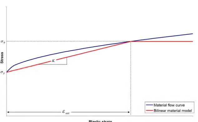
In the first sensitivity analysis conducted in Section 6.1 a second type of isotropic hardening was used. There bilinear hardening was defined,

pl H K   0pl ₀ where , and max K K  wherepl ₀ (4.2)

where H is a material constant, pl is the equivalent plastic strain and 0 is a saturation strain.

The data used to define K is provided in Table 4.2 and the way in which the material parameters were identified is illustrated in Figure 4.2.

Figure 4.2 Illustration of how parameters for the bilinear hardening models were obtained. The blue curve represents a material flow curve and the red curve represents the bilinear hardening model.

4.3.2 Kinematic

With kinematic hardening the concept of a backstress is introduced and the yield surface translates with accumulated plastic strain. In this study linear kinematic (Ziegler) hardening was used because it is available as a model within the ABAQUS material library. In this model the yield surface is

defined by, 0 ) (     f X _y f   (4.3)

where X is a backstress tensor whose rate of change is defined by,





The data used to define X for the two kinematic hardening parameter sets is shown in Table 4.2.

sat

Table 4.2 Mechanical properties for stainless steel (316). Temperature (degrees Celsius) Yield stress (MPa) [19] Stress at a strain of 0.01 (MPa) [19] Stress at a strain of 0.1 (MPa) [19] Estimated strain rate sensitivity exponent, m 20 217 266 558 0* 200 121 188 387 0.0210 400 110 142 320 0.0178 600 75.9 125 364 0.0742 700 169 220 371 0.117 800 140 159 244 0** 900 69.3 89.4 149 0.0515 1100 33.1 41.7 69.1 0.128 1300 18.6 22.1 31.6 0.176

* The strain rate sensitivity was so small that it could not be accurately estimated from the available charts. It was therefore set equal to 0.

** The measured strain rate sensitivity was actually negative (due to DSA) but to avoid numerical difficulties during FE analysis its value was set equal to 0.

4.3.3 Mixed isotropic and kinematic

Mixed hardening was used in Chapter 5 and defined as per the nonlinear isotropic/kinematic hardening model available in ABAQUS. This model allows both expansion and translation of the yield surface. Here the yield surface is defined by Eqn (4.3). The isotropic and kinematic hardening components y and X are, however redefined,





 and b are additional material parameters and y,0 is the initial yield stress. The data used to define

mixed hardening for 316H stainless steel [23] is shown in Table 4.3 for the temperature range of interest.

Table 4.3 Mechanical properties for stainless steel (316H) [23]. Temperature (degrees Celsius) Yield stress (MPa) C (MPa)  Q∞ (MPa) b 20 280 18,800 150 69.1 53.2 200 210 17,241 150 80.5 46.1 400 200 12,752 150 81.8 12.5 600 175 12,374 150 99.8 37.7 850 108 0 150 0 0.25 1000 55 0 150 0 0.25 1400 4.5 0 150 0 0.25

4.3.4 Perfectly plastic (non strain hardening)

This model was used in Section 6.1 and is the simplest form of plasticity because the material does not strain harden. A von Mises yield surface is used and the flow stress is simply defined as the yield stress,

y



₀  (4.6)

Values of the yield stress used for the perfectly plastic model are available in Table 4.2. 4.3.5 Viscoplastic

The viscoplastic model was used in Section 6.2 and allows for the strain rate sensitivity of the flow stress to be accounted for. In this study isotropic hardening is assumed. In the case of austenitic stainless steel the yield stress tends to increase with an increase in strain rate and this effect may be modelled as follows, m ref ref y _              (4.7)

where ref is the flow stress at the reference strain rate

1 2

10 

 s

ref

 . Values for m were obtained using a least squares estimate where the flow stress at a strain of 0.1 was specified in Eqn (4.7) for strain rates between 5x10-3 and 10s-1. The values obtained for m are shown in Table 4.2.

5

SIMULATIONS AND VALIDATION TO MEASURED RESULTS

The weld residual stress modelling procedure described in Section 3.2 was applied to two cases (see Table 5.1) where residual stress measurement results are available from the literature for well documented weld mock-ups. The purpose was to compare the weld residual stress predictions from different hardening models with experimental measurements. In this section three material hardening models were chosen for analysis:

 Isotropic with a fully defined flow curve using data for 316 published by Lindgren et al [19].  Linear kinematic using data for 316 published by Lindgren et al [19].

 Mixed, as specified by Leggat et al [23] for 316H stainless steel.

Axi-symmetric modelling was used in all cases. The welding inter-pass temperature was assumed to be room temperature, which will tend to over-estimate residual stresses if the actual in-pass

temperature is higher. The annealing temperature was set to 1400 °C.

Further sensitivity studies with respect to the assumed hardening model are presented in Section 6. The residual stress profile has been measured in detail for these cases by neutron diffraction, deep-hole-drilling, and surface-hole drilling techniques, and documentation of the cases are found in [24-26].

Table 5.1: Case definition.

Case No. Name Pipe thickness t [mm] Pipe radius to thickness ratio Rin/t Groove type Number of passes Weld type Heat input * [kJ/mm] Material (parent/ weld) Repair weld depth [mm] 1 SP19 19 10.5 V 15 (*) MMA 1.35 316H/316 L ~ 2 S5VOR 65 2.8 V 45 MMA 2.4 316H/316 L ~

Measurements will always give a mean average value of the stress in a gauge volume in the material, and with some uncertainty with respect to the distance from the fusion line, see discussion in [27]. Considering this, care must be taken when choosing evaluation paths from finite element models. In the present study these evaluation paths were chosen to lie along the centre of the measruement gauge volume. Stress distributions obtained in this way are suitable for comparison with experimental results provided the stress gradient perpendicular to the gauge volume is linear or nearly linear. This

evaluation method was judged to be suitable for the present case. The measurement data compared to in Figures 5.5-5.8 were taken from an actual weld mock up and reflect measurements along a given path from the actual three dimensional pipe. As discussed in [28], the residual stress field in a multi-pass pipe butt-weld has a clearly-defined periodic variation along the pipe circumference, in addition to weld pass start and stop effects. This variations must be kept in mind when comparing experimental and numerically calculated weld residual stress fields.

5.1 Case 1 – Intermediate pipe

In the first case a medium thick-walled pipe having Rin/t = 10.5 was analysed. The geometry and the

sequence of the weld passes are shown in Figure 5.1. Two through-wall paths were selected for

evaluation of the through-wall residual stress distribution; these are also shown in Figure 5.1. The pipe geometry is given in Table 5.1. Detailed information on the weld mock-up fabrication and welding process parameters were taken from [24], [25] and [29]. The finite element mesh is shown in Figure 5.2.

Since the previous report, more detailed information has been obtained regarding the welding

geometry and sequence [29]. The finite element model has been updated accordingly. Most notably, the three capping passes have been modelled, because inclusion of a weld cap is known to have a significant influence on the residual stress distribution.

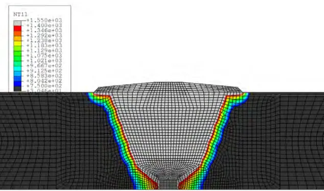
The peak temperature experienced during welding is shown in Figure 5.2. The fusion zone for the 14-pass weld is indicated by a temperature level exceeding 1400 °C. The HAZ is indicated by the temperature band ranging from 750 °C to the fusion line (1400 °C).

Figure 5.1: Geometry, definition of sequence of welding and finite element mesh for Case 2.

Figure 5.2: Fusion zone and HAZ. Maximum temperature experienced during the welding. The locations with a maximum temperature exceeding 1400 °C are plotted with gray colour and the locations with a maximum temperature lower than 750 °C are shown with black colour.

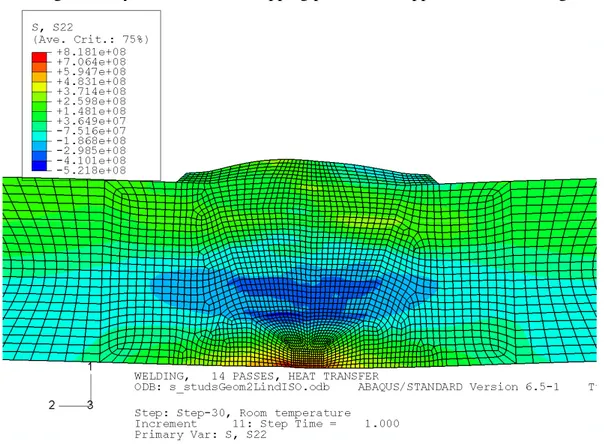
The predicted axial and hoop residual stress distribution, for the isotropic hardening model are shown in Figures 5.3 and 5.4. From Figure 5.4 it is seen that the stress field is

most significantly the fact that the capping passes were applied from left to right.

Figure 5.3: Axial residual stress for the medium thick-walled case 2 weld at 20 °C (unit Pa). Isotropic hardening was specified for this figure.

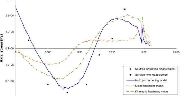
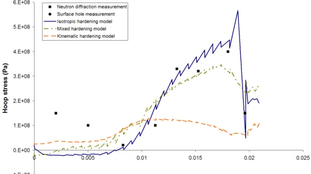
The predicted residual stress distributions along Path1, as indicated in Figure 5.1, are compared with neutron diffraction measurements documented in [24, 25], as shown in Figures 5.5 and 5.6. This path lay mostly outside of the weld zone in parent metal, except towards the outer surface of the pipe, where it came into contact with the weld cap. The three modelling results shown correspond to the kinematic, isotropic and mixed hardening models. Best agreement is observed for the isotropic hardening model – where for the axial stress good agreement is observed for both the shape and the magnitude of the residual stress distributions. For the hoop stress good agreement is also obtained, except on the inner surface of the pipe where the stress magnitude is underestimated. With the kinematic hardening model the magnitude of the stress peaks was greatly underestimated for both the axial and the hoop stress. As might be expected, the distribution for the mixed hardening model lay between the isotropic and kinematic cases. A discussion regarding the observed differences for the different hardening models is given in Section 5.3.

Figure 5.5: Case 1. Comparison of predicted axial residual stress (S22) along Path 1 (defined in Figure 5.1) for different hardening models. Available experimental data is also plotted.

Figure 5.6: Case 1. Comparison of predicted hoop residual stress (S33) along Path 1 for different hardening models. Available experimental data is also plotted.

The predicted residual stress distributions along Path 2 from Figure 5.1 are shown in Figures 5.7 and 5.8. This path began on the inner surface of the pipe in parent material but then crossed into weld material a little less than half way through the thickness. For Path 2 the best agreement with experimental data for the axial stress is obtained for the isotropic hardening model. The best agreement for the hoop stress is obtained for the mixed model. Note also that the hoop stress is overestimated using the isotropic model once the path crosses into weld material.

As with Path1, the kinematic hardening model tends to underestimate the stress magnitude for both the axial and the hoop stress.

Figure 5.7: Case 1. Comparison of predicted axial residual stress (S22) along Path 2 (defined in Figure 5.1) for different hardening models. Available experimental data is also plotted.

Figure 5.8: Case 1. Comparison of predicted hoop residual stress (S33) along Path 2 for different hardening models. Available experimental data is also plotted.

5.2 Case 2 – Thick-walled pipe

A thick-walled pipe case having Rin/t = 2.8 was analysed. Although new material hardening models

have been defined, the geometry and the finite element mesh are unchanged from the previous study; the mesh in and around the weld is shown in Figure 5.9. The sequence of welding (a total of 45 passes) is defined in the figure. Two through-thickness paths were selected for evaluation in this study, namely those labelled HAZo and CL, as indicated in Figure 5.9.

The peak temperature during welding is shown in Figure 5.10, illustrating the predicted fusion zone and the heat affected zone shape and sizes.

Figure 5.10: Maximum temperature experienced during the welding. The locations with a maximum temperature exceeded 1400 °C are plotted with gray colour and the locations with a maximum temperature lower than 750 °C are shown with black colour.

The final residual stress distribution at 20 °C is shown in Figures 5.11 and 5.12 for the axial and hoop residual stress components, respectively. Note that the axial residual stress distribution in Figure 5.11 has a different shape to that seen in Figure 5.5 (Case 1). This can be attributed the difference in

geometry of the pipes. In this case the radius to thickness ratio of the pipe is smaller (2.8 versus 10.5), such that there exists a stronger mechanical constraint to suppress the ‘tourniquet’ deformation within the weld that led to high tensile stresses on the inner surface of the pipe in Case 1.

Figure 5.11: Axial residual stress for the thick-walled case 2 weld at 20 °C (unit Pa). Isotropic hardening was specified for this figure.

The predicted residual stress distributions along the path HAZo (see Figure 5.9) are compared for the isotropic, kinematic and mixed hardening models in Figures 5.13 and 5.14 against experimental measurements, taken from [13]. The best agreement with experimental data is obtained for the

isotropic hardening model, although good agreement is also obtained for the mixed hardening model. Both the predicted axial and hoop residual stresses correlate well with the measured data as shown in Figures 5.13 and 5.14. This is in contrast to the results reported in phase one of this project, where the hoop stress was greatly overestimated at the outer surface of the pipe. The improvement in the stress estimate may be attributed to the more comprehensive material data set used in the later stage of the project. In contrast to the isotropic and mixed hardening models, the stress magnitude was

underestimated for the kinematic hardening model - a similar trend that was observed for case 1 (19mm thick pipe) .

Figure 5.13: Case 2. Comparison of the predicted axial residual stress (S22) along path HAZo (from Figure 5.9) with the measured.

Figure 5.14: Case 2. Comparison of the predicted hoop residual stress (S33) along path HAZo (from Figure 5.9) with the measured.

Stress distributions along the weld centreline (path CL) were also compared in Figures 5.15 and 5.16 for the different hardening models against experimental measurements. The distributions have a similar shape to those along path HAZo, although for path CL the stress magnitudes are greater. Once again, the best agreement with experimental measurements is obtained for the isotropic and mixed hardening models.

Figure 5.16: Case 2. Comparison of the predicted hoop residual stress (S33) along path CL (from Figure 5.9) with the measured.

5.3 Comments on the choice of hardening model

In the previous two sections weld residual stress fields were predicted from FE welding simulations using isotropic, kinematic and mixed hardening models and the distributions were compared with available experimental measurements. Two girth weld geometries were considered. It is possible to make some observations about the suitability of the different material hardening models.

The best predictions of the axial stress were obtained from the isotropic hardening model, regardless of geometry or measurement location. For the hoop stress the best predictions were obtained from the mixed hardening model, although the isotropic model also gave good agreement (except for Case 1 - 19mm thick pipe, along Path2). In contrast the kinematic hardening model systematically

underestimated the magnitude of the weld residual stress field for both the axial and the hoop stress. Based on these results it is advisable to use an isotropic hardening model since it gives the closest overall agreement to experimental measurements. In those cases where the mixed hardening model gives better agreement, namely prediction of the hoop stress for the 19mm thick pipe, the isotropic model predictions tend to be excessively tensile, guaranteeing conservatism for fracture mechanical assessments based on a critical crack size (but not those based on the leak before break principle). There are also a number of questions which remain unanswered:

1. How can the results published by Ogawa et al [2] be explained? There they reported only a small difference in predicted weld residual stress fields when isotropic, kinematic and mixed hardening models were considered. It may be that their results can be reproduced by

modifying the hardening models and defining a very small saturation strain - a method that has been used in the past, for example, by [4]. The implementation of such an isotropic model is the topic of the first sensitivity study.

2. Rate effects have not been considered in this study – can the implementation of a viscoplastic model affect the shape of the weld residual stress field? This is the topic of the second sensitivity analysis.

3. In terms of predicting residual stress fields, the most problematic case was the hoop stress for the 19mm thick pipe. It is not directly apparent why this case is problematic. This point is reserved for the final discussion.

6

SENSITIVITY ANALYSES

6.1 Use of bilinear hardening where there is a small saturation strain

There are some instances in the literature [4] where hardening models have been implemented

differently to the present study such that hardening is only allowed up to a predefined saturation strain, of the order of 0.01. This type of model is applied here for isotropic hardening. It is unclear whether this approach gives improved predictions. To test the effect, the 19mm girth weld geometry from case 1 is chosen and three different material hardening models are defined:

 Perfectly plastic (no strain hardening). This model is used as a reference.

 Bilinear isotropic. Bilinear hardening is defined and the saturation strain is set to 0.01.  Kinematic (Ziegler) hardening.

The resulting stress distributions are shown in Figures 6.1 and 6.2 for the axial and hoop stresses, respectively. Firstly, it is clear that this implementation of the hardening model does not give an improved prediction of the weld residual stress – there is poor agreement with the experimental measurements for the new isotropic hardening model. When compared with the perfectly plastic reference case, the isotropic model gives higher stress magnitudes on the axial and the hoop stress plots. The kinematic model, on the other hand, displays a small amount of hardening on the axial stress plot but softening on the hoop stress plot. It is therefore concluded that the alternative material hardening implementation does not give a better prediction of the weld residual stress field than the isotropic model with flow curves that are fully defined for the temperature range of interest. It may be possible to improve the predictions of the bilinear isotropic model by adjusting the yield stress and hardening modulus, although such changes are likely to be geometry dependent.

Figure 6.1: Case 1. Comparison of the predicted axial residual stress (S22) along Path1 (from Figure 5.1) with the measured, when an alternative implementation of the hardening models is used.

Figure 6.2: Case 1. Comparison of the predicted hoop residual stress (S33) along Path1 (from Figure 5.1) with the measured, when an alternative implementation of the hardening models is used.

6.2 Effect of introducing viscoplasticity

The second sensitivity study concerns rate effects - and whether it is important to consider them. A viscoplastic model has the potential to represent two behaviours:

1. Stress relaxation that may occur during heating and cooling that is induced by bead addition.

2. Strain rate hardening that occurs during initial weld bead addition since there exists a high thermal gradient and therefore a relatively high rate of deformation during this phase.

For the second sensitivity study the Case 1 geometry (19mm thick) was chosen and the following material hardening models were used:

 Isotropic, where flow curves at different temperatures are fully defined in tabular form.  Viscoplastic where tabulated isotropic hardening is defined together with a strain rate

sensitivity.

Figure 6.3: Case 1. Comparison of the predicted axial residual stress (S22) along Path1 (from Figure 5.1) with the measured, when a viscoplastic hardening model is considered.

Figure 6.4:. Case 1. Comparison of the predicted hoop residual stress (S33) along Path1 (from Figure 5.1) with the measured, when a viscoplastic hardening model is considered.

7

DISCUSSION AND RECOMMENDATIONS FOR FUTURE

WORK

The focus of this study was to determine which type of material hardening model should be used in weld residual stress simulations. The results indicate that an isotropic hardening model that is

temperature sensitive and has fully defined strain hardening curves gives the best agreement with weld residual stress measurements.

One instance in which the isotropic model did not give good agreement with experimental data was for the hoop stress for the 19mm thick weld (Case 1). In this case the hoop stress was underestimated on the inner surface of the pipe and overestimated on the outer surface. It is difficult to identify the cause of this discrepancy since for the 65mm thick weld (Case 2) good agreement for the hoop stress was obtained. The key difference between these welds is geometrical. In Case 1 the radius to wall thickness ratio is 10.5 whereas for Case 2 it is 2.8. It may be that 2D axisymmetric weld simulations with higher Rin/t ratios are overconstrained in the hoop direction due to the fact that the weld bead is

effectively added instantaneously around the entire pipe circumference. Further investigation of this is required.

It is also not directly obvious why the isotropic hardening model gives better overall agreement with experimental measurements than the mixed hardening model. It must be noted that two different sources of data were used for the isotropic and mixed models in this study and this may have

contributed to the discrepancy in predictions. When defining a mixed hardening model it is difficult to delineate the relative contributions of isotropic and kinematic hardening and for the model used it may be that a greater isotropic hardening component should have been specified. There also exist two issues relating to the formulation of the mixed hardening model available in ABAQUS:

1. The range of temperatures experienced during welding simulation is vast and the mixed model used in ABAQUS was probably not originally intended for such an application. When rapid changes in temperature occur, as with bead addition, it is possible that the backstress X is not properly represented. In the present mixed model the value of the backstress does not change with a sharp change in temperature. Therefore when there is a sudden temperature rise from an equilibrium state (e.g. bead addition) the magnitude of the backstress is overestimated. This problem could be overcome by reformulating the model in the framework of the theory of thermal activation [31].

2. It is well known that the mixed model must be calibrated for a specific strain range [20] and that different material parameters are obtained if cyclic tests are conducted over a different strain range. In a multipass weld it is unlikely that the strain range will remain constant for the history of a specific bead and, to the authors’ knowledge, the strain history has not been well quantified. It is therefore not immediately clear which strain range the mixed hardening material parameters should be based upon. An alternative approach would be to obtain or

in this study were taken directly from experimentally determined stress strain curves. It is

acknowledged that with engineering judgement it may be possible to modify the models such that they give similar results, although such an approach is not beneficial to the improvement of the welding simulation method.

7.1 Recommendations for future work

Any engineering model has to be validated to experiments and measurements in order to demonstrate that its output is representative for the reality. Weld residual stress calculation models are complex and involve several physical processes and accompanying assumptions, so it is important that they are validated experimentally. Large improvements have been made by the new weld residual stress modelling procedure developed in the different stages of this project. However, there still exist some questions that are not fully resolved. As discussed above, well grounded assumptions are fundamental in order to attain a reliable prediction model. Some issues in weld residual stress modelling still need further investigation in order to confirm and settle some basic assumptions and approximations. Further model refinements should preferably be validated to residual stress fields measured using the latest versions of the measuring methods.

The recommendations for future work that have been made below relate to the material properties used in welding simulation. There are also other areas of improvement, such as further improvement of the heat source calibration procedure. For each identified issue a tangible proposal is given for how to solve the problem.

1) Investigation of the mechanical overconstraint that arises from instantaneous addition of

a weld bead during 2D weld simulation. The degree of this overconstraint can be estimated

by calculating the amount of cooling around the circumference that occurs during the addition of a bead. It may then be possible to adjust the coefficient of thermal expansion in the hoop direction to relax the constraint accordingly. Such a procedure could also be applied as part of the development of a 2D method to simulate repair welds, where only a fraction of the

circumference undergoes contraction due to the addition of weld beads.

2) Testing to obtain temperature-dependent flow curves and cyclic stress strain data for

important welding alloys. One barrier to improved weld residual stress simulation is the

availability of material data for the temperature range of interest. Cyclic stress-strain data is generally lacking for all of the important welding alloys and even good quality monotonic data is missing for materials such as alloy 82 and 182. A testing program to determine material properties for common welding materials would be of direct benefit to the accuracy of weld residual stress simulations. It would also allow development of material models for use in welding simulation.

3) Observation of grain size distributions within weld regions and development of a

recrystallization model to predict the grain size and the grain size dependence of the flow stress. This recommendation relates to the specification of material properties in the weld

region which is a topic of current discussion [12, 32] and was raised in the first phase of this project [1]. At present no comprehensive method is available to properly represent material behaviour in the weld and the heat affected zone. Efforts have been made to measure the properties after welding but by this stage the material is already plastically strained. High temperature thermo-mechanical test results could be used to develop a model to predict the

grain size and the grain size dependence of the flow stress for welding alloys. This would allow the more accurate material properties to be specified within the weld region and the heat affected zone.

8

CONCLUSIONS

The aim of this study was to determine which material hardening model gave the best agreement with experimentally measured weld residual stress distributions. Two girth weld geometries were

considered.

As a preliminary step some improvements were made to the existing welding simulation procedure:  Monotonic stress strain curves and a mixed hardening model for 316 stainless steel were

sourced.

 More detailed information was obtained regarding the geometry and welding sequence for the Case 1 weld (compared with phase 1 of this project).

Following the preliminary step welding simulations were conducted using isotropic, kinematic and mixed hardening models. The isotropic hardening model gave the best overall agreement with experimental measurements; it is therefore recommended for use in welding simulations. The mixed hardening model gave good agreement for predictions of the hoop stress but tended to underestimate the magnitude of the axial stress. The kinematic hardening model consistently underestimated the magnitude of both the axial and hoop stress and is not recommended for use.

Two sensitivity studies were also conducted. In the first the effect of using a bilinear isotropic hardening model with a saturation strain of 0.01 was evaluated. This model was not capable of accurately predicting the weld residual stress field and its use is not recommended.

In the second sensitivity study, the effect of defining a viscoplastic model was evaluated. For

predictions of the axial and hoop stress the viscoplastic model was found to give slightly lower stress peaks, although the effect was sufficiently small that the increased complexity and computational cost of defining such a model probably outweighs the benefits. It was noted that a similar effect could be obtained by lowering the annealing temperature.

Following the outcomes of this study three recommendations for future work are made:

1. An investigation of the possible overconstraint of 2D axisymmetric girth weld simulations in the circumferential direction. This effect may lead to overpredictions of the magnitude of the hoop stress for pipe geometries where there is a large radius to diameter ratio.

2. Testing to obtain temperature-dependent flow curves and cyclic stress strain data for important welding alloys. This would be of direct benefit to the accuracy of weld residual stress

simulations, particularly for alloys where little material data is available.

3. Development of a model to accurately predict the material properties within the weld region and the heat affected zone.

9

REFERENCES

1. Zang, W., Gunnars, J., “Improvement and validation of weld residual stress modelling

procedure,” Inspecta Technology Research Report No. 50002550-1, Rev 1, 2008.

2. Ogawa, K. et al, “The measurement and modelling of residual stresses in a stainless steel pipe

girth weld,” Proceedings of 2008 ASME pressure vessels and piping division conference, PVP

2008-61542, 2008.

3. ABAQUS Analysis User’s Manual Volume III: Materials, Version 6.7, SIMULIA, Providence, 2007.

4. Hedblom, E., “Simulation of multipass welding to reduce intergranular stress corrosion

cracking,” Licentiate Thesis, Department of Mechanical Engineering, Luleå University of

Technology, 2000.

5. Brickstad B, and Josefson L, “A parametric study of residual stresses in multi-pass butt-welded

stainless steel pipes,” Int. J. Pressure Vessels and Piping, Vol. 75, pp 11–25, 1998.

6. Price J.W.H., Ziara-Paradowska A.M, Joshi S., Finlayson T., C Semetay C., Nied H., “Comparison of experimental and theoretical residual stresses in welds: The issue of gauge

volume, “Int. J. Mechanical Sciences, Vol. 50, pp 513-521, 2008.

7. Rosenthal, D., “Mathematical theory of heat distribution during welding and cutting,” Welding Journal, Vol. 20, pp 220-234, 1941.

8. Friedman, E., “Thermomechanical Analysis of the Welding Process using the Finite Element

Method,” Journal of Pressure Vessel Technology, Trans. ASME, Vol. 97, pp 206-213, 1975.

9. Goldak, J., Chakravarti, A. and Bibby, M., “A New Finite Element Model for Welding Heat

Sources,” Met. Trans. B, Vol. 15B, pp 299-305, 1984,

10. Taylor, G.A. et al., “Finite volume methods applied to the computational modelling of welding

phenomena,” Proceedings of Int. Conf. on CFD in the Minerals and Process Industries,

CSIRO, Melbourne, Australia, 1999.

11. Eagar, T.W. and Tsai, N.-S., “Temperature Fields Produced by Traveling Distributed Heat

Sources,” Welding Research Supplement, pp 346-355, 1983.

12. L. Edwards, et al., “Advances in Residual Stress Modeling and Measurement for the Structural

Integrity Assessment of Welded Thermal Power Plant,” Advanced Materials Research, Vols.

41-42, pp 391-400, 2008.

13. S.K. Bate, P.J. Bouchard, P.e.J. Flewitt, D. George, R.H. Leggatt and A.G. Youtsos, “Measurment and Modelling of Residual Stress in Thick Section Type 316 Stainless Steel,”

Welds, Proc. Sixth International Conference on Residual Stresses, ICRS6, pp 1511-1518,

17. Material specification, “Specs: 316, 316L & 317L,” Sandmeyer Steel Company, 2009,

http://www.sandmeyersteel.com/images/316-316L-317L-Spec-Sheet.pdf

18. Albertini, C. et al, “Dynamic Mechanical Properties of Austenitic Stainless Steels – Fitting of

Experimental Data on Constitutive Equations,” Proceedings of the 7th International Conference on Strutctural Mechanics in Reactor Technology, Division L, pp 53-62, 1983.

19. Lindgren, L., et al, “Dislocations, vacancies and solute diffusion in physical based plasticity

model for AISI 316L,” Mechanics of Materials, Vol 40, pp 907-919, 2008.

20. Van Eeten, P.J.C., “Cyclic plasticity of a stainless steel: investigation of cyclic plasticity of

316L through experimental and numerical methods,” Masters of Science Thesis, Department

of Solid Mechanics, KTH University, Sweden, 2005.

21. Ohmi, Y. et al, “Constitutive modelling of proportional/nonproportional cyclic plasticity for

type 316 stainless steel applicable to a wide temperature range,” Materials Science Research

International, Vol 1, No 4, pp 247-253, 1995.

22. Ohmi, Y. et al, “Formulation of constitutive models for cyclic deformation of type 316

stainless steel at high temperature,” The Japan Society of Mechanical Engineers, No. 95-0074,

pp 98-105, 1995.

23. Leggat, N. A., et al, “Numerical methods for welding simulation – the next technical step,” Proceedings of 2008 ASME pressure vessels and piping division conference, PVP 2008-61498, 2008.

24. Bouchard, P.J., “Validated residual stress profiles for fracture assessments of stainless steel

pipe girth welds,” Int. J. Pressure Vessels & Piping, Vol. 84, pp 195–222, 2007.

25. L. Edwards, G. Bruno, M. Dutta, P.J. Bouchard, K.L. Abbott and R. Lin Peng, “Validation of

Residual Stress Predictions for a 19 mm thick J-preparation Stainless Steel Pipe Girth Weld using Neutron Diffraction,” Proc. Sixth International Conference on Residual Stresses, ICRS6,

pp 1523-1526, Oxford University, Institute of Materials, UK, 2000.

26. S.K. Bate, P.J. Bouchard, P.e.J. Flewitt, D. George, R.H. Leggatt and A.G. Youtsos, “Measurment and Modelling of Residual Stress in Thick Section Type 316 Stainless Steel

Welds,” Proc. Sixth International Conference on Residual Stresses, ICRS6, pp 1511-1518,

Oxford University, Institute of Materials, UK, 2000.

27. Price J.W.H., Ziara-Paradowska A.M, Joshi S., Finlayson T., C Semetay C., Nied H., “Comparison of experimental and theoretical residual stresses in welds: The issue of gauge

volume,” Int. J. Mechanical Sciences, Vol. 50, pp 513-521, 2008.

28. Dong, P., “Residual Stress Analysis of a Multi-Pass Girth Weld: 3D Special Shell Versus Axisymmetric Models,” Journal of Pressure Vessel Technology, Vol. 123, pp 207-213, 2001. 29. Bouchard, P.J., et al, “Measurement of the residual stresses in a stainless steel pipe girth weld

containing long and short repairs,” International Journal of Pressure Vessels and Piping, Vol

82, pp 299-310, 2005.

30. Tomota, Y., et al, “Application of the Kocks-Mecking model to tensile deformation of an

austenitic 25Cr-19Ni steel,” Acta materialia, Vol 49, No 15, pp 3029-3038, 2001.

31. Kocks, U.F., et al, “Thermodynamics and kinetics of slip,” Progress In Materials Science, Vol 19, 1975.

32. M. Kartal, et al., ”Determination of Weld Metal Mechanical Properties Utilising Novel Tensile

Testing Methods”, Applied Mechanics and Materials, Vols. 7-8, pp 127-132, 2007.