Measurement of the bearing capacity of roads : A comparison between four measuring methods

STATENS VAG- OCH TRAFIKINSTITUT

National Swedish Road and Traffic Research Institute

MEASUREMENT OF THE BEARING CAPACITY OF ROADS

-A COMP-ARISON BETWEEN FOUR ME-ASURING METHODS

by

Olle Andersson

REPORT No. 61 A

Stockholm 1975

STATENS VAG- OCI-I TRAFIKINSTITUT

National Swedish Road and Traffic Research Institute

MEASUREMENT OF THE BEARING CAPACITY OF ROADS

A COMPARISON BETWEEN FOUR MEASURING METHODS

by

Olle Andersson

REPORT No. 61 A

Stockholm 1975

VTI. Report No; 61;A 'Table 'Table 'Table ' CONTENTS

SUMMARY

INTRODUCTION

MEASURING EQUIPMENT

TEST LOCATIONS RESULTS T el Table 2 Table Table Table Table 'Table 10 MEASURING CAPACITY

-SELECTION OF MEASURING SYSTEM

CONCLUSIONS

ACKNOWLEDGEMENT

REFERENCES

Figures 1 - 24 . Page 10 12 13 13 15 15 16 18 19 20 21 . 22 23 , t h yr v u», I: my. .. _

SUMMARY

The present report deals with a comparatiVe investigation of four different methods for measurement of_the bearing capacity of roads, 'namely V

- conventional static plate hearing test (SP)

deflection measurement at transient drop hammer loading (DH) ' deflection measurement at heavy vibrator loading (HV)

- determination of dynamic elastic modulUs from measurements of propagation of elastic waves caused by a light vibrator (LV).

All methods were tried regurlarly on eight test sections on eight

occasions distributed over one climate cycle. These test sections were a selection of five test sections of a test road at Brista near

.Arlanda airport and three sections on abandoned parts of the shunt

road 849 between E4 and E18 in the same area. lsolated meaSurements

'were also made in the city of Malm , Sturup airport near_Malm6 and E18 bypass near Urebro, mostly full depth type of pavements.

Based on the main sequence of tests a judgement of the four systems with respect to

- technical features

- measuring capacity

- measuring costs

has been made.

Seasonal variations were significant only on thick bituminous pavements and pavement on organic soil. On such measuring objects there is also av significant difference between static and nonstatic tests. Where high

measuring capacity in mileage is important Swedish experience is not

in favour of static measurements, including Benkelman beam systems,

neither of existing wave propagation measuring systems. This work was sponsored by the Swedish Road Administration.

MEASUREMENT OF THE BEARING CAPACITY OF ROADS A COMPARISON BETWEEN FOUR MEASURING METHODS

INTRODUCTION

The following report deals with the results of measurements of the bearing capacity of roads at eight different locations and at eight different times during one climate cycle, the measurements being performed by four different instruments:

- conventional static plate bearing tester (SP)

- drop hammer (DH) I

- heavy vibrator (HV)

- light vibrator (LV).

By the three first instruments a load is applied to the road surface

via a circular plate (diameter 300 mm) and the deflection of the road surface is measured. In the present mea3urements the DH och HV deflections were measured at the centre of the plate. The SP deflections were measured

on opposite edges of the plate..By the light vibrator technique the phase' shift of elastic surface waves was measured at frequencies mainly in the

_interval'40 - 1000 Hz. From these data diapersion diagrams (rate of wave

propagation/wave length) were worked out for assessment of the layer

elastic moduli. The composite elastic modulus of each pavement was

computed by the Chevron programme for multi-layer elastic system analysis. »The deflections obtained by the first three methods were used for

computation of the nominal elastic modulus according to the formula,

E = 1.5 P/Tfrd

II

where P applied load

' r radius of loading plate

.deflection.

The load P was in the DH-test 44 RN and in the SP and most of the

HV-measurements 40 RN.

The modulus values were used exclusively in order to make possible a compariSon with the results frOm the light vibrator measurements and should be considered mainly as normalized deflection values.

The purpose of the Study was to obtain a comparison between deflection

measurements made at; i

- static loading - impact leading - cyclic loading

all at simulated truck load level and also the dynamic elastic modulus resulting from analysis of propagation of elastic waves, when measurements

are made on the same occasion, at the same measuring points, the main source of variation in bearing capacity being change due to climate. The .measuring points were selected to represent the five subgrade classes

referred to in the Swedish Road Administration thickness design

specifications and the most common types of road base. Suitable road ' sections were found in the vicinity of Stockholm. Measurements made at a few other locations in Sweden, where two or more of these instruments were used at the same measuring points have also been-included in the

report.

MEASURING EQUIPMENT

The static plate bearing tester used is a hydraulic jack mounted at the-rear end of a conventional truCk, Scania vabis L 8046. The oil pressure actuated piston carries at its lower end a universal joint, to which the load plate is attached. The deflection is measured at two opposite points

on the plate close to the edge of the plate by means of dial gauges

attached to a 2.5 meterslong reference bar. On stiff pavements a 4 meters.

long reference beam has also been used, but the difference between the

measurements Was negligible. The loading routine implies application of the load by 10 kN increments, 1/2 minute apart. At full load the pressure is released to zero, followed by application of full load as soon as the dial gauges show a constant reading. The rebound deflection taken as the difference between dial gauge reading at full load and after the

censecutive deloading, is noted at consecutive load-deload cycles until two consecutive rebound deflections differ by less than 5 Z. The latest rebound deflection is then recorded as the final deflection reading. The measurement was made at two points, separated 15 - 30 meters, on each

test section.

The drop hammer used is of Danish design (1), and works by dropping a 150 kg weight on to the upper end of a spring, whose lower end is.

Vattached to the loading plate. The load pulse is therefore theoretically'

a half sine wave of about 25 ms duration. In the centre of the loading plate there is a hole which makes possible the attachement of a deflection measuring device to the naked road surface. The deflection measuring

device was in these measurement a seismometer type LVDT deflection meter (2) designed and built at our institute, which gave the peak deflection

reading on a peak voltmeter. Loading was at each measurement repeated

'several times, until the difference between two consecutive readings

was approximately 0.01 mm. The reading was then assumed to repreSent

rebound deflection. The loading plate diameter was in all measurements

300 mm. A rubber carpet was attached to the plate for pressure equilization. The heavy vibrator used in the measurements is a Losenhausen 2000/15-75 machine foundation vibration resistence tester, which is hung up inside

a city bus. Through a square hole in the floor of the bus the vibrator can be lowered hydraulically to the road surface. To the lower face of

the approximately cubically shaped vibrator is attached a heavy steel

rod, carrying at its lower end a load_and deflection measuring cell,

the bottom of the cell being shaped as a circular loading plate of 300 mm diameter. The cell and the load measuring system have been designed.in' the same way as in the Shell heavy vibrator (3) and was built according to drawings kindly supplied by the Shell Laboratory in Amsterdam. The deflection measuring device is a geophon, manufactured by Sensor NV, Holland. The geophon is attached to a 12 mm steel rod, which protrudes

downwards through a hole in the loading plate and is spring mounted to this plate inside the cell. When the whole assembly is lowered to the

road surface the steel rod is.therefore pressed inwards (upwards) against 1

its spring load and.is therefore forced against the naked road surface, the force being sufficient to ascertain contact with the road surface at any vertical acceleration expected.

The vibrating mechanism is an unbalanced double rotor, which gives a resultant vertical centrifugal force adjustable, by setting of the

unbalance weights, between zero and 4 tons double amplitude, the force

varying sinusoidally. The frequency of the vibrator can be varied continuously in the interval 15 r 75 Hz. In the measurements reported

here the frequency was set at about 20 Hz. Load and deflection signals are processed electronically in a homebuilt operation amplifier-device and their peak value measured by a Br el & Kjaer Type 2409 electronic voltmeter. The setting of the unbalance of the vibrator is stepwise,

and therefore in the present measurements the unbalance was set as close

as possible to giving the intended load amplitude (40 kN), and final. adjustment was done by adjusting the frequency. Due to the flexibility of the rOad pavement the vibrator plus road forms a vibrating elastic system, which transmits forces greater than the centrifugal force and which varies with frequency. Preset load at a preset frequency cannot be implemented by this equipment due to the stepwise unbalance setting. The wave propagation equipment used was a Ling Dynamic Systems vibrator

and amplifier, HP function generator, double beam oscillosCope and ' various homebuilt electronical compOnents for amplification and frequency control. Detection was made by a Philips geofon. Type PR 9260. For

frequencies above 1000 HZVa piezo detector was uSed..Detection of

half-wavelengths was done manually. Since the measurements are very time- 0

consuming, some reduction of the.procedure had to be done, and measuremente; above 1000 Hz were omitted, except in a few cases, the missing modulus

of the top layer obtained by using known modulus-temperature curves. For analysis of the diapersion diagrams the technique suggested by Jones (4) was used.

TEST LOCATIONS

.

'

»

Cy:

The main test sequence Was carried out on five different pavements along road 263 at Brista near Arlanda airport and on three pavements on road 849, a shunt road between E4 and E18, joining E18 at the Staket junction. The measurements on road 263 at Brista were made on a test road with different road bases, which was built in 1963 (5). Five sectiOns of this

test road were used, denoted according to the following list: (Figures

within ( ) correspond to the section number in (5)).

.Section . rRoad Base ' , ' Subgrade

1. (MM) (1) I Hot mix grouted macadam Till

2. (CM) (3) Mortar stabilized macadam Sandy clay

3. (CG) (4) Lean concrete - . Sandy clay

4. (BG) (7) Bitumen stabilized .Clay

5. (OB) (8) 'Unbound graVel Clay

. The subbase was in all sections gravelous sand - sandy gravel. A schematic section of these pavements is shown in fig. 1. The test sections on road 849 were located on untrafficked parts which were left available after the road was rebuilt and partly realigned in 1970. The sections were denoted as follows:

Section Road Base 7 . I Subgrade

6. (Staket) Bitumen grouted macadam i

Till-7._("Sawmill") Bitumen grouted macadam Gravel layer on till

8. ("Swamp") Unbound gravel Silty till on peat, swampy area

The "sawmill" section is located close to a sawmill and is partly used

for lumber storage and has been trafficked by heavy timber trucks after

the section was abandoned by ordinary traffic. A schematic section of

these pavements is shown in fig. 2.

Test locations outside the main sequence which were not tested by all the four methods and on isolated_occasions were the following.

yalms, iralsgatanz City street with full depth asphalt pavement on a clay subgrade. The details are shown in fig. 3.

Malmo, Kaglingevagen: City street with full depth asphalt pavement on

a clay subgrade.

§tgrup: Various pavements (runways, taxiways and aprons) on Malmo airport at Sturup. Details are shown in fig. 4.

Qrebrg_22: City bypass along road E18 at Crebro. The details are shown

érlanda: The first section of road E4 north of Arlanda junction. The measuring points cover two_different pavement structures, one having

10 cm bitumen stabilized road base upon crushed rock subbase, the other ' one having 15 cm.bitumen stabilized road base upon a gravel subbase. The road was a neWbuilt motorway.

The measuring points in the main sequence were selected according to fig. 1 and 2. In each sections two groups of three points each

were selected, the groups being 15 - 50 meters apart and the

points-within each group 3 meters apart. Drop hammer and heavy vibrator measurements were made at each point, whereas static plate bearing tests were made only at the middle point in each group of three. Wave propagation measurements were made along lines through these points.-Eight test locations at eight occasions therefore added up to 384 moduli each by the drop hammer and heavy vibrator methods and 128

moduli by the static plate bearing test. The wave propagation measurement had to be omitted on two occasions, and the total number of wave '

propagation moduli was therefore 96. This amounts to 992 modulus values altogether in the main sequence.

The main sequence started in March 1973 and ended in April 1974. The intention was to catch one frost breaking state. The winters of the respective years were however exceptionally mild, and measurements of frost penetration showed no frost in 1974. Some occasional frost penetration had probably taken place in 1973 before the start of the measurements. Measurement schedule:

No. l 2 3 4 _5 - r 6 7 '8

March May June July September October November April

At all measurements the air temperature and the temperature at various depths were measured (table 1).

RESULTS

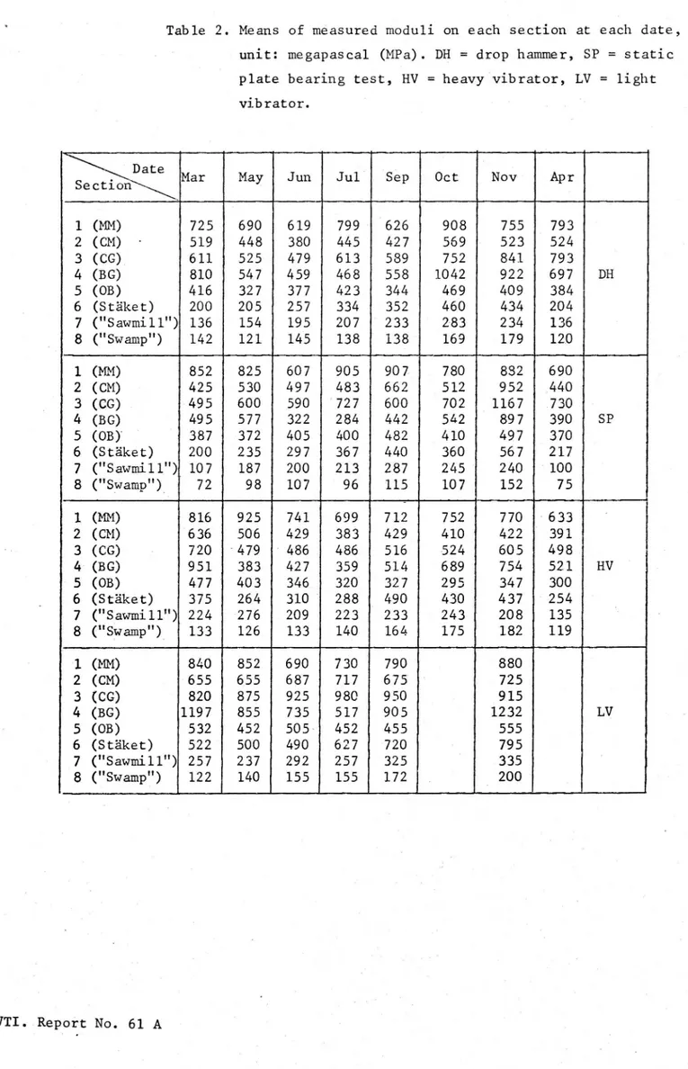
The mean modulus value of each section at each measuring date obtained

by each measuring method is listed in table 2. The modulus values are

given in megapascals (MPa) = Newtons-per square millimeter. The drop hammer and heavy vibrator values are means of.SiX points, the static

plate bearing values are means of two points and the light vibrator

values are means of two lines.

It is observed that the Brista sections show higher values than the. other three sections throughout, which could be expected when considering -the pavement class on these test roads. The "swamp" section shows the

lowest values throughout. Of the Brista sections the highest values are

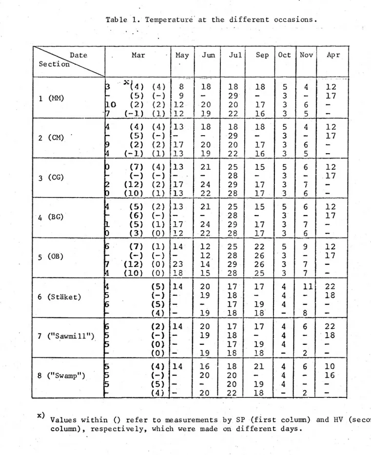
Table 1. Temperature at the different occasions.

Date . Mar - May Jun Jul Sep Oct Nov Apr

Section - ' _

3

(4) (4)

8

18

18

18

5

4

12

1034)

~

(5) (-)

9

-

29'

. 3

-

17

_

11)

(2) (2) 12.

.20

20

17

3

6

-~7 (~1) (1)112 .19 22 16 3 5

4

(4) (4) 134

18

18.

18'

5

4

12

2 (CM) - (5) (-) : 7 - v 29 - 3 17

9

(2) (2)*17

20.

20

17

3

6

4

( 1) (1) 13 _ 19

22

16

3 I 5

~

,

o

(7) (4) 13

21

25

15

5

6

12

3 (CG)

'7

('7') ('7) ~ --

-

28

-

3

-

.17

»

2

(12) (2) 17

24

29

17

3

7

o

(10) (1) 13

22

28

17

3

6

~

4

(5) (2)f13

21

25

15

5

6

12

1 (Ba)

-

(6) (-) g" -

-

28

-

3'

-

17

.

1

(5) (1);17

24

29

17

3

7

~

0

(3) (0) 12

22. '28

17

3

6

-V 61'

(7) (1) 14 v12

25

22

5

9

12

»5 am)

-

(-) (~)

12,

28

26

'3

'17

7 '(12) (0) 23

14

29-

26 v 3

7

4

(10) (O)'18'

15

28 ' 25

3

7

4

(5) 14

20

17*

17

4

11

22

6 (staket) 5 ( ) "' 19 18 . - 4. 18

6

(5) -

-,

17 - 19

4

-

- '

~

(4)'-

19

18

18 .-

8

-6

(2)'14.

2o

17

17

4

6

22

7 ("Sawmill") 5

(- ) .-

19-

18

-

4

-

'18

' 5

(0)

17

19

4

-~

(0) u'

19

18. 18

-

2

-. s

(4) 14

16 - 18

21

,4

6,

10

8 Cswmmw)

5

'(e) -

20,

20

4

-

16»

5

(5) e

~

20

19

.4 .

(4)'-

20 A 22

18

- . 2

x) Values within () refer to measurements by SP (first column) and HV (second

column), respectively, which were made on different days.

.9.

Table 2. Means of measured moduli on each section-at each date,

unit: megapa3ca1 (MPa). DH = drop hammer, SP = static

plate bearing test, RV = heavy vibrator, LV = light

vibrator.

2\;;:::3323:i\ Mar May Jun Jul . Sep Oct Nov Apr

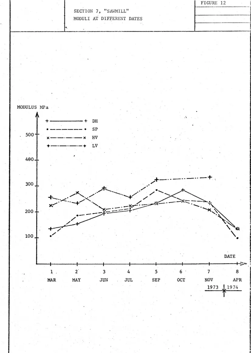
1 (MM) 725 690 619 799' 626 908 755 _ 793 a 2 (CM) - 519 448 380 445 427 569 523 524 3 (CG) 611 525 479 613 589 752 841 793 4 (BC) 810 547 459 468 558 1042 922 697 DH 5 (OB) 416 327 377 423 344 7469 409 384 6 (Staket) 200 205 257 334 '352 460 434 204 7 ("Sawmill") 136 154 195 207 ' 233 283 234 136 8 ("Swamp") 142 121 145 138 138 169 -179 120 1 (MM) 852 825 607 905 907 780 882 690 2 (CM) 425 -530 497 483 662 _512 952 .440 3 (CC) . 495 600 590 '727 600 702 41167 .730 4 (BC) 495 577 322 284 442 542 897 390 SP 5 (OB) ' 387 372 405 400 482 410 497 370 6 (Staket) 200 '235 297 367' 440 360 567 217 7 ("Sawmill") 107 187 200 213 ' 287 245 240 "100

8 ("swamp")~ F 72

98

107

- 96

115

107

152

75

1 (MM) 816 ' 925 741 699 712 752 770 '633 2 (CM) '636 506 429 383 429. 410 422 I 391 3 (CC) 4 720 '479 486 486 516 524 605 498 4 (BC) 951 383 427 359 514 689 754 521 HV - 5 (0B) 477 403 346 320 327 295 347 300 6 (Staket) 375 264 310 288 490 a 430 437 254 7 ("Sawmill") 224 ~276 ..209 223 233 243 208 135 8 ("Swamp")A 133 126 133 140 164 175 182 119 1 (MM) 840 852 690 730 790 880 2 (CM) 655 655 687 717 675 725 3 (CG) ' 820 875 925 980 950 915 4 (BC) 1197 855 735 5173 905 1232 LV 5 (OB) 532 452 505 452 455 555 6 (Staket) 522 500 490 627 720 795 7 ("Sawmill") 257 237 292 257 325 335 8 ("Swamp") 122 140 155 155 172 I 200

10.

recorded from section 1 (hot mix grouted macadam base), the.LV values excepted. This is probably not caused by a high base modulus but rather a stiffer subgrade. The "sanill" values (section 7) are unexpectedly low. This section was originally intended to represent a sandy gravel

subgrade. The gravel layer on top of the till subgrade, however, appeared to vary considerably in thickness along the road, and at the actual

.measuring points it was fairly thin, and the till had a high water content throughout the season. This explains_the comparatively low

values recorded at this section.

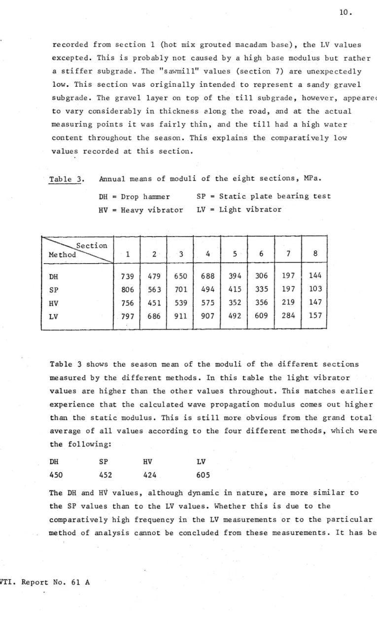
' Table 3. Annual means of moduli of the eight sections, MPa. DH = Drop hammer SP = Static plate bearing test RV = Heavy vibrator LV = Light

vibrator-Section . Method ' l . 2 .. 3 . 4 . 5' 6 7 . 8 DH 739 479 650 688 394 306 197 144 SP 806 563 701 494 415 335 197 103 HV 756 451 539 575 352 356 219 147

LV

797

686

911 , 907

492

609

284

157

Table 3 shows the season mean of the moduli of the different sections measured by the different methods. In this table the light vibrator values are higher than the other values thrOughout. This matches earlier experience that the calculated wave prepagation modulus comes out higher than the static modulus. This is still more obvious from the grand total

average of all values according to the four different methods, which were

the following:

DH ' SP HV LV

450 452 424 605

The DH and HV values, although dynamic in nature, are more similar to

the SP values than to the LV values. Whether this is due to the

comparatively high frequency in the LV measurements or to the particular method of analysis cannot be concluded from these measurements. It has been

ll.

argued that the light vibrator causes much lower stress levels than the

other three testers, and the reason for the higher wave prepagation modulus-is the high initial slope of-the stressrstrain curve of soil materials. Triaxial cyclic tests of typical road building materials in Sweden do n0t_confirm this View, the stress-strain curves being progressive rather than regressive. It should also be noted that the

moduli computed from the two slower dynamic tests (DH and HV) are purely ~ nominal, since they are not derived from inertia influenced stress-strain behaviour of the measuring object.

The seasonal variation of the moduli listed in table 2 is illustrated

diagramatically in figures 6 - 13. Although it is not the purpose of this work to study the seasonal variation of bearing capacity, a few ' observations will be made. In_most of the measuring objects dealt with

the seasonal variation is not considerable in comparison to the

randOm-Vlike fluctuations. The BC section (fig. 9) shows the U-shape which could

be expected from a road base whoSe bearing capacity is sensitive to the variation with temperature-of bitumen viscosity. The same shape is not Iobserved in section 1, although the road base is in this section also

bitumen bound. This observation supports-the statement made above, that section 1 derives most of its comparatively high bearing capacity from the particular subgrade, the stabilization of the road base being of less importance. Sections 6 -'8 whose seasonal variations are plotted in figures 11 - 13 show an increase in modulus throughout the year and a return to lower moduli the following spring. This is true for most of the measuring methods. The increase during the year is most probably I caused by.a decrease in moisture content of the pavement and subgrade. .In section 6 (Staket) the wave prepagation values are much higher than.

the other groups, and in section 8 ("swamp") the static bearing capacity

curve is lower than the other curves, which criss-cross. The high level

of the wave propagation curve in section 6 reflects a rather high value' of the till subgrade modulus derived from the dispersion curve. It Could be argued, that_this being the case, a Similarly high level would result

in section 1, having a similar subgrade. In this section the pavement is, however, considerably thicker, and the low frequency waves do not reach

the same depth as in section 6. This illustrates the importance ofta correct interpretation of all the details of the disperSion curve.

12

In section 8 the comparatively low level of the static plate bearing modulus illustrates the high deflection of swampy systems under static, loads. Apparently the yielding water soaked bed offers inertia

preSistence against oscillatory loading, which gives a lower deflection amplitude than is given time to occur under static load.

For a comparison of the numerical values of the moduli of the different measuring methods the values of table 2 were used for calculation of ratios of moduli according to different measuring methods. Four numbers, taken two-at a time, can give twelve different ratios, six of which are the inverse value of the other six. Six/ratios were therefore

calculated, and the grand total_average over sections and season

gave the following values

DH/SP

HV/DH'

LV/DH

HV/SP

LV/SPCI

LV/HV

This sequence suggests quite similar numerical values of heavy vibrator and drop hammer moduli and also rather similar numerical levels in comparison of these moduli with the static moduli. The almost 50.2

higher level of the light vibrator moduli is again illustrated. Calculation .of ratios and averaging.Can actually be made in many different ways,

' leading to different end results. Conclusions from these figures should therefore be drawn_with great care.

The correlation matrix involving the four measuring methods and based on two individual readings from each test section and from the whole

test period is shown in table 4. It is noted that the correlation

Table 4. Correlation coefficients

DH

SP

HV

LV

0.84OV 0.901 0.863

DH

0.760 0.769

SP

0.781'

av

coefficients involving drop hammer are fairly high, all above 0.8, the, highest value pertaining to the DH-HV correlation. The difference between VTI. Report No. 61 A

'13.

this correlatiOn coefficient and any other correlation coefficient in the list is statistically significant. Differences between the nearest lower coefficients are not statistically significant. This indicates a closer correlation between the two methods DH and HV than between other methods tested. The accompanYing regression coefficients and their standard deviations are listed in table 5. Regression coefficients closest to 1 and

Regression coefficients.and standard deviations

Table-5.

Independent variable DH SP HV LV 0.65 0.88 0.61 DH -0.043 0.044 0.037

1.08

0.95

0.70

SP -0.072 0.084 0.06 Dependent 0.92 0.60 0.56 variable HV -' 0.046 0.053 0.046 1.23 0.85 41.08

LV

0

-0.074 0.073 0.089

. Table 6. Standard deviations around regression lines, MPa. Independent variable DH SP HV LV

DH . -

117 I

94

110

SP 152 ' - 182 179

Dep8ndent

HV

96 .

145

~

139

variable . LV 156 197 193 f

v11. Report No. 61 A

14.

the smallest standard deviations belong to the DH-HV correlation,' confirming the indication that these two methods have the closest

relation.

The standard deviation about regression, listed in table 6, shows the smallest values in the DH/HV regression.

A.plot of section-mean values of.DH and HV readings is shown in figure 14, and a plot of means of readings from all sections (the remaining variation being only season) is shown in figure 15. In this plot the 95 Z confidence

limits are also drawn. For a further analysis of the different

contributions to variation in the results the whole bulk of raw data

and seleCted parts of them were subjected to analysis of variance. The purpose of this analysis was primarily to find the stochastic variation inherent in the four different methods tested and the significance in-differences between methods. "Inherent variation" in this connection

means the part of the ObServed variation, which cannot be aSCribed

to any one of the variables studied.

An analysis of variance based upon the mean modulus at eaCh test section

Ion each occasion and measured by the methOds DH, SP and HV gave

Significant influence of test sections and seasons but not method.

For a teSt of the influence of method this approach is, however, too

blunt an instrument. This is so partly because seasonal variations with test sections are systematic in a sense not fully taken care of by the analysis of variance. Consider for instance figure l3, where the SP curve is obviously different from the other three curVes. Statistical confirmation of this observation has been obtained by taking differences between simulataneous moduli from SP and DH and testing the difference

between zero and the mean of these differences by the t-test. The test_

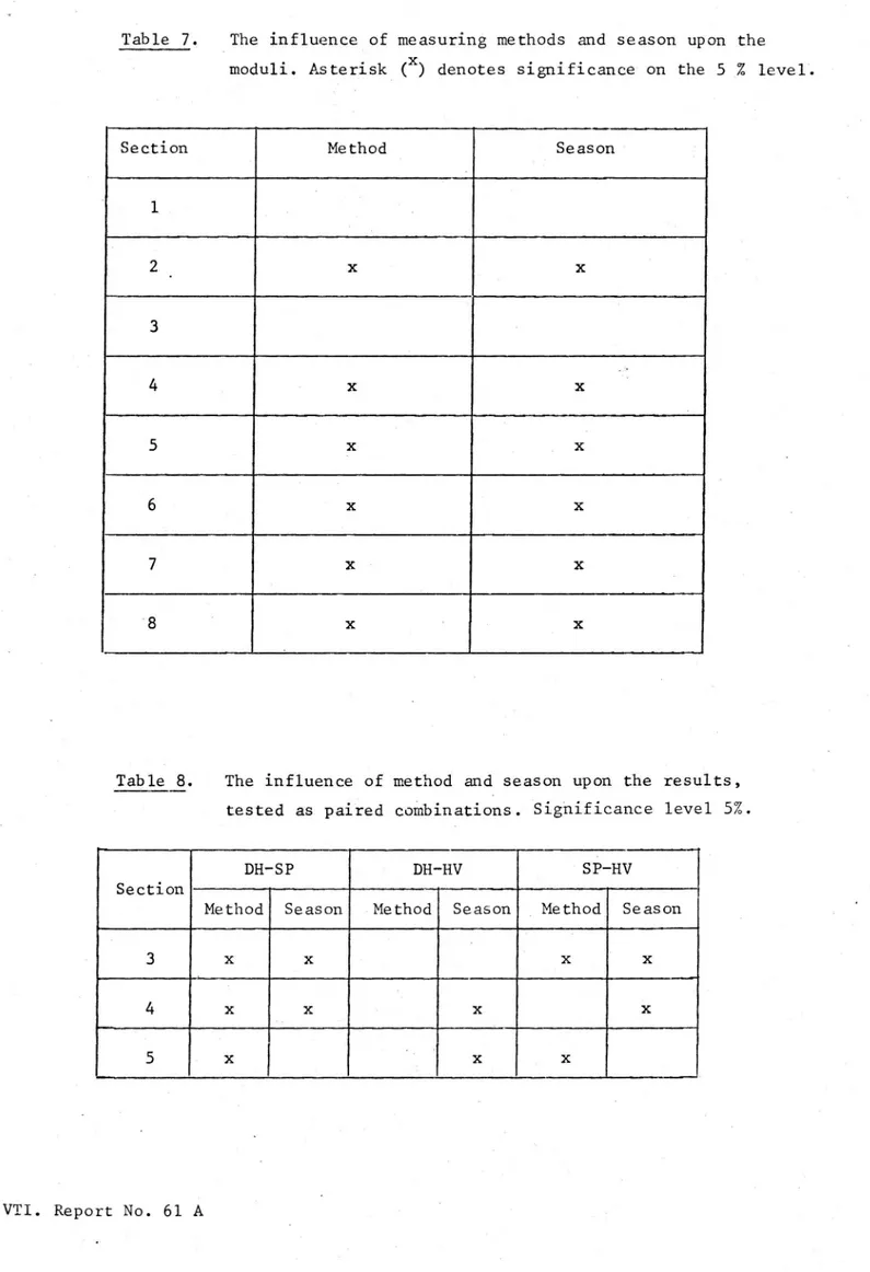
gave high significance. Similar tests of more limited sets of data have occasionally given significant differences. In table 7 are listed results

of analysis of variance made separately for.each test section. The

' components of variation due to season and method were tested. The asterisks denote significant variation on the 5% level, which was obviously prevailing_in most cases when considering one test section

at a time.

15.'

Table 7. The influence of measuring methods and Season upon the moduli. Asterisk (X) denotes significance on the 5_Z level;

Section Method , Season

1 2 x x 3 4 x X 5 x x 6 x X 7 x x 8 x x

Table §. The influence of method and season upon the results,

tested as paired combinations. Significance level 5%.

DH-SP

.DH HV

SP-HV

Section

Method Season -Method Season 7 Method_ Season

3 x x x x

4 x x x x

S x x x

16.

A more broken down_test. limited to two methods at a'time and one test' -section at a time, comprising three test sections, is shown in table 8.

The test seetions.were those with the cement stabilized base, the bitumen stabilized base and the non stabilized base (sections 3, 4

and 5). The DH-HV comparison did in no case give significant influence of method. Of the remaining six comparisons significance due to methodf was recorded in five cases. Of the total of nine comparisons,

significance due to seasonal changes was recorded in six cases. Indications.of various kinds point towards a rather wide agreement between drop hammer and heavy vibrator mOduli. whereas_comparisons involving other methods show greater discrepancy. 3

my» 7 z

. 1 .'0'

Table 9.

Inherent variation in different methods 0n different sections (MPa). The.standard-deviations were calculated

from the various variance compontents.

Method

DH

»

_

SP

HV

.

LV

' . - Coeff. ~4 "Coeff. - Coeff. 4 Coeff.

Seetxon E G of var. E O of var., E G of var. E O of var.

3 648 88 0.14 702 111 0.16 539 72 0.13 r r

-4 » 688 54 0.08 494 135 0.27 574 96 0.17 907 39 0.04. 5. 393 19 .0.05 416 '41 0.10 352 34 0.10 492 46 0.09

4 8

144 20

0.14

103 .20 0.19

147 21 0.14' 157 17 0.11

An approaCh to isolation of the variation inherent in the different methods was attempted by analysis of variance of the original readings

from each instrument on four separate test sections as shown in table 9. The sections were number 3, 4, 5 and 8, and the readings from the six

different points measured by DH and HV, the two different points meaSured . by the SP and the two different lines measured by LV were processed

in-the analysis. Each variance was divided into in-the three components caused: by variatiOn in

¥location of the point along-the section

~season and

residue.

17.

In table 9 are listed - grand mean

f stanard deviation based upon residual variance

- Coefficient Of variation.

Comparison of the means shows a fair agreement on section 5 (unbound base) and some agreement between plate loading methods on section 4

(bitumen stabilized base). It is noteworthy that the means of section 4 are higher than those of section 3 (cement stabilized base) when measured by dynamic methods. The static plate bearing method shows a considerably higher value on section 3 than on section 4, a discrepancy which is

probably typical for the static type of measurement. The residual standard deviation varies considerably when making comparisons between sections but not so much when comparing methods on the same sections. This is

partly caused by the difference in-means, since the coefficients of lvariation do not vary appreciably between sections. All the basic

conditions of the analysis of variance are obviously not fulfilled, and general conclusions regarding the residual variance cannot be drawn. An inherent coefficient of variation of the single observation in the region 10 r 20 Z can, however, be considered as a reasonable estimate. The standard deviations (o) of LV in table 9 are small in comparison

to that of other methods. This is a consequence of the method of calculation of the LV modulus, in which the modulus of the wearing course was given constant values at each temperature.

For more reliable analysis of the variance among different points on the same section a different approach was tried. The actual standard deviation and mean of the six readings on each section at each measuring occasion were calculated. The results are listed in table 10 and are for the sake of better illustration plotted in figure 16. This analysis was. limited to the two methods DH and HV, since these were the only two methods by which six-readings were taken each time. The six readings Vwere distributed along the road c0vering a distance of some 30 meters.

It is seen in table 10 that the standard deviation varies considerably,

which probably reflects the seasonal variation of the bearing capacity.

Each standard deviation displayed in the table is composed of inherent instrument variation and variation along the road. A separation of the

VTI.

18.

yzab1e_10. Drop hammer and heavy vibrator. Mean (six points) and

standard deviation on different occasions, sections 3, 4 and 5. Unit: MPa.

Mean Standard Deviation Range Occasion -DH HV DH HV DH HV Section 3 1 610 719 89 141, 215 355 - 2 524 478 74 59 195 115 3 461 485 47 56 130 140 4 612 485 94 111 _255 305 5 588 515 98 84 265 205 6' 751 523 156 65 360 150 7 840 605 247 108 530 255 8 792 497 56 49 160 100 Section 4 1 809 950 84 146 165 405 ' 2 545 382 74 59 215 '135 3 459 426 22 58 V 65 175 4 468 358 33 34 95 90 5 557 514 41 - 30 100 85 6 1041 688 ' 94 107 205 270 7 921 753 114 153 325 425 8 696 520 59 79 130 235 Section 5 l 415 476 45 37 110 105 ' 2 326 403 32 85 90 235 3 376 345 38 41 105 105 4 423 319 51 ' 38 130 100 5 343 326 35 38 ' 90 110 6 »469 295 67 16 150 40 7 408 346 62 47 150_ 115 8 383 300 32 60 80 155

two components is not feasible, but comparison-With table 9 would suggest-that the major part of the variation is inherent in the measuring systems. A closer analysis at some isolated points showed a rather close correlation

between the composite modulus of the pavement and the modulus of the subgrade.

Modulus variations along the road are sometimes assumed to reflect the

occurence of weak spots. Such variations would, however, not Show tlie recovery during the season, and therefore, in the present study,

' o o o 0

along the road variations can be conSLdered as caused mainly by

19.

variations in the subgrade modulus. The Brista test road, although ten years old, is still in very good condition and has shown no evidence

of weak Spots apart from those that occurred due to temperature cracking

in the very beginning.

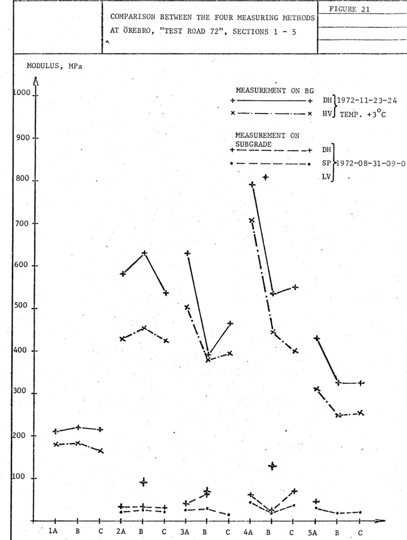
Results of measurements made at other test locations outside the main sequence are shown diagrammatically in figures 17 - 24. Measurements

were made mainly by DH and RV and at some places by SP. Mostly there

is an obvious conformity.between the curves relating modulus to measuring point, although levels do show some discrepancy. This is especially true for the SP moduli, cf for instance figure 17, where the similarity in the shape of the curves is unmistakable, but the SP level is appreciably

lower than the DH and HV levels. This is a full depth pavement on a

rather weak subgrade, and most of the bearing capacity is probably due

to the properties of the bitumen bound pavement. The discrepancy is

therefore in all probability a result of the particular resistance of bituminous systems to dynamic loading. The DH level is somewhat higher

than the HV level, which is true for most pavements of this type.

In figure 23 the ratio of DH to HV moduli is plotted against section

number. A systematic variation appears to be at hand. It should be noted that the sections were tested in random order, which rules out

the influence of factors varying with current time. The pavement. _structures are shown in figure 5, which_reveals that sections 2 -~5

are full depth pavements, some of them being built on a lime stabilized

subgrade. Sections 1 and 6 -IlO are mainly unstabilized rock embankments.

A similar result is obtained also from other sections, including those of the main sequence (sections 4 and 6). The results suggest a systematic

difference between transient loading and oscillatory loading, resulting

for instance from the difference in the distribution of bonding strength with respect to inertia in the two types of pavements.

MEASURING CAPACITY

This report has so far been limited to the purely physical aspects of

the four methods tested. In selection of methods for practical

application in measurement of the bearing capacity of roads decisions also have to be based upon time consumption and cost, these two factors

20.

being to a considerable extent related to each other. Advantages and

ldisadvantages also vary considerably with the type of application intended. Two types of application will be considered, based upon the

instruments actually used in the present study. Other versions of these

instruments may have different time and labour consumption. Application (1)

considered here is continuous measurement along a primary road at 50 meters

interval with the purpose of surveying road networks. Application (2) is 1 km of paved road, measured at 50 meters intervals serving for instance as a.basis for decision about strengthening priority.

as

2.1.1.

.113

.131

appl (l) measurem./hr 3 12 '12 l

appl (2), no of days 1 1/2 1/2 1/2 4 l/2

manpower-required l l l 2 I

automization no yes yes no

The last line denotes the feasibility of having the measurement automated

in the sense that push-button controls can be arranged in the driver's

'seat for remote operation of the instruments. Automization of the heavy vibrator is a routine matter and is known in market instruments of this

kind, whereas automization of the drOp hammer requires development work. SELECTION OF MEASURING SYSTEM

The present study was made partly in order to give a basis for selection' of appropriate meaSuring systems for different purposes in Sweden. In these considerations systems based on the Benkelman beam were also included, the conclusions being based upon earlier experience of the

Benkelman beam in Sweden.

For occasional applications, where high measuring capacity is unimportant,

any one of the methods considered_can be recommended, with the exception

of the Benkelman beam in gravel road or thin pavement application- In such applications the Benkelman beam showed erroneous results due to lateral

movement of unbound material between the twin wheels.

>

In large scale applications, where high measuring capacity in mileage is a prerequisite, the drop hammer and heavy vibrator systems can be

21.

recommended, provided the drop hammer system is developed to the push-button operation stage. Such a development has not yet been done but is

feasible. Fatigue properties of certain vital parts of the drop hammer

system are not yet fully known. The heavy vibrator and semi-heavy vibrator systems are on the other hand fully developed and marketed.

No semi~heavy vibrator was included in the present study, and their correlation with heavy vibrators of the type included remains to be found out. The deflectographs have too small measuring capacity in-mileage for the applications considered.

CONCLUSIONS

Measurement of the nominal elastic modulus of various road pavements by three plate bearing methods, implying impact loading, static loading and oscillatory loading at simulated traffic level and by the wave

propagation method at low loading level has shown a noteworthy agreement

betWeen the four methods both with regard to magnitude and seasonal variation of moduli. Systematic differences were observed, which were mostly expected

- wave propagation moduli had a higher level than the others, but in grand total average only about 50 Z

- static plate bearing moduli were lower than the others, when meaSured on heavy bituminous pavements

- static plate bearing moduli were lower than the others when measured on a swampy subgrade

- impact loading gave higher moduli than oscillatory loading on pavements with bituminous bound road base and vice versa on pavements with

unbound crushed rock road base

~ on conventional pavements with well-graded unbound base the differences

between methods was not very pronounced H

I

- the variation of modulus with season was appreciable only on pavements

with bitumen bound base and pavements on a very wet subgrade

VTI.

22.

~ the seasonal variation was most pronounced with the dynamic methods~ ~ variation of_subgrade modulus along a pavement had an appreciable

influence upon the composite modulus

* the inherent variation of the single observation was 10 - 20 Z of the mean, when measured at impact and oscillatory loading.

ACKNOWLEDGEMENT

The work reported here was sponsored by the Swedish Road Administration. The measurements in the main sequence were planned in cooperation with Olle Tholén and the soil investigation was done by Nils Lundgren. The measurements outside the main sequence were made in conjunction.with other research work, mainly sponsored by the Road Administration, the' Administration of Civil Aviation and the City of Malmo. The measurements

were made by staff of the road base group of the institute and were most of the time led by Lennart Carlbom. The mathematical analysis and

the compilation of the report was made in cooperation with Lennart Djarf.

The Benkelman beam studies were performed by Sven Engman, who supplied

the basis for the conclusions regarding its applicability. The contributions of my coworkers is greatly acknowledged.

23.

REFERENCES

1. -Bohn A, et a1: "Danish Experiments with the French Falling Weight Deflectometer", Proceedings, Third International Conference on

the Structural Design of Asphalt Pavements, Vol 1, London 1972, pp 1119-1128.

2. Tholén O: "Provning och utveckling av apparatur for stBtbelastning med fjadrad fallvikt", Statens vag- och trafikinstitut, Internrapport

nr 107, Stockholm 1973.

3. Klomp A J G and Niesman Th W: "Observed and calculated Strains at

Various Depths in Asphalt Pavements", Proceedings, Second International

Conference on the Structural Design of ASphalt Pavements, Ann Arbor ~

1967, pp 671-672.

4 a. dones R: "Following Changes in the Properties of Road Bases and Sub-bases by The Surface Wave Propagation Method",_Civ Eng and

P W Rev, London 1963, 58 (682), 613, 615, 617, (683), 777-80.

4 b. Jones R: "Thickness and Quality of Cemented Surfacings and Bases -1 Measuring by a Non-Destructive Surface Wave Method", Civ Eng and

Rev, London 1965, 60 (705), 523, 525, 527, 529.

5. Drbom B; "Barlagerprovvagen vid Brista", Statens Vaginstitut, Specialrapport nr 31, Stockholm 1965.

6. Tholén O: "Barighetsbestamning med fjadrad fallvikt , Statens vag-och trafikinstitut, Internrapport nr 173, Stockholm 1974.

7.- -Transportation Research Board, "Pavement Rehabilitation: Proceedings

of a Workshop", Transportation Research Board, Report No. DOT-OS-AOOZZ,

Washington 1974.

r.

LA

NE

-,

-I

_

',

.

O -. . I v. -« v F un k . c a n . ~ 7 . 3 . . " f . . . c a n . b ut m t o ut m -uC -n wm uw-0 % H I . ' 9 . m e cul l-~n -n . w a n . m wwm a n . -o c u. m b -. -ya m -m -m -c n . p m uI II I-b n -m w-m a n . k -f F l a wJ " -' . -' -W U . -l - v-. -l -~w ~* . -~* .I 9-1-0-Tr0

1+-Odd-LL¢I

HO

RI

ZO

NT

AL

VI

EW

OF

SE

CT

IO

NS

,

LE

NG

TH

OF

SE

CT

IO

N

10

0

M

_

|

_1

.

2

.

'

.

3

4

h

I

'

5

3 5 + 0 . 0 0 , V2 ,5 ;C m AC , v, V W Z I S c h AC ' Al l) CE II HA IL 1/ 7 10 cm OB 2, 5 cm AC v 2, 5 cm AC 4, 5 cm AC I r ,r v. vrx .r rr r7 v r r 1'71 A U T W 1f '1 / 1 I; 7 lf 2 * J-ém AC ' 1' 7, / 7/ '

15

cm

36

.

18

cm

BA

SE

GR

AV

EL

.

f i l f x f f ' ? ' 4' ' 1 # 4 A l 1 5 -c m C G I S C M E M

.5

cm

EA

SE

GE

AV

EL

v =9"4%

GR

AV

EL

LY

SA

ND

-G

RA

VE

LL

Y

SA

ND

.

"

GR

AV

EL

LY

_S

AN

D

GR

AV

EL

LY

SA

ND

'

SA

ND

Y

GR

AV

EL

.J'. __,ra~ Q nun-urn. .«wm

.Olp qr-D'O- np A nno -mos -._u

.-3: U GxL -O

\

02:1 31998 P\OOI=I»91958

.

-f

'

r:

®\

II

NT

ER

ME

DI

AT

E

'/

1'

\\

-CL

AY

."

'

,

/

.

\

'/

SA

ND

Y

TI

LL

CL

AY

EY

sI

LT

_

I

r-E f--I H {-4

,\ , I

.Ji...

:3}-.

V

/

\

.

.F

IN

E

CL

AY

\

"

. I A/

h'

uZ

O

1

'

'

'

I

.S

OL

ID

GR

OU

ND

.

i

_

x

. ia

_w ' Mum onmv-vcu-n Q

5 a I _ . . v

LO

NG

IT

UD

IN

AL

S

CT

IO

N~

'

>

v

'

"

'

-_ E , &. . , . . IV ,E ;, . . AL L LENG TH S AR E GI VE NIN ME TE RS ,»T EE OR IGIN AL WE AR ING CO UR SE IS -' t ' ' , -, é , ,'_ I F ER JD To. TH E RO HAS BE EN . P OS ITIO N 0F ME AS URIN G PO IN TS . «1 1L 1: b. OF MEASURING POINTS

TEST ROAD AT BRISTA , SECTION 1~5 . SUBGRADES, PAVEMENTS AND POSITION

EE

SU

EE

AC

ED

ON

CE

AN

D

AN

UN

KN

OW

N

:

'

,

_'

.

.

*

SP

\V

.LV

SP

7'

L?

TH

IC

KN

ES

S

HA

S

BE

EN

WO

RN

AW

AY

.

'

I-,

I

\

' 1; m m II I-u. ~ -( Vi ew A . M f . . . m o m O -I V 3+ 3 yi n m * ¥ A_ _A . :; 43 i, ' N . 1 3+ 3 <9 1 m a . . . C u-m 4 }1

{NJ

15 -30 ~n -4 1 . 4 5 t h a.. , o n ! a n a n " . In m N. » wwwm - v-1 3 ? M m g 1 * M y i j vm m h m 3 . 7 »; E u-w g+ ¢r .. ¢, m. twa ng . m k ' f éy um vw. m4 p w-a m «t n w4 m ym ' m ua s n wn w 4a a a m . » m4 : w 2~ b' PQ t we n t -v. o rr vwwi ws m 9. ; 3 » 3w - a- w-r W 4 i m ii . a w no a n r ur n: v In t-m = A N W W W " n in m t FIGURE 1

50 m

T

:1

9%

'

??7

6 (STA KE T) 2. 5 cm AC 5 ! I

3-3}'

7{§3

m

a 1 ' 0 j o I a...

J-

O ' I

6

cm

GR

OU

TE

D

MA

CA

DA

M

4

'

20 cm GR AV EL A A A v. TI LL O O *: -- o o 50 m . I I I ' | J 5a

_if

£

3

m r 3 m 3' m, m c d- v-JL n o 7 (S AW MI LL ) 2. 5 cm AC f r r». d o J r A . A 4 , : , , , " ; , p L -; ; AA ej 5 cm G R O U TED M A C A D A M AI S ' 20 cm GR AV EL ! W l

....J

V C L A YEY T I L L ~. .

.JI.

.JLlw-I.-~..~C no .Jho dH-I 8 (S WA MP ). n

l-oqr umo "Jr. col-+0

d*

-*

axa

l~i

s'

;~m

ri

sm

-"

-4 -4 A 25 cm GR AV EL w w 35 cm C L A Y E Y TI LL

WI

TH

CO

AR

S

MA

TE

RI

AL

J

A A A W E T O R G A N IC MA TE RI AL( BE AT ) I MEASURING POINTS,

SUBGRADES AND LOCATION OF

SECTIONS 6+8

PAVEMENTS,

FIGURE 2 _ov.(wh

i

LMb ' " FIGURE 3

AMIRALSGATAN

. n SUBGRADE AND PAVEMENT

N S F -N a n d , 7 . «-, gr um pyx y, ..

LOCATION OF MEASURING POINTS

I

«M

p

-9

All lengths are given in meters

v. 28;.7 1g, 1,3; 2c; 1+5

#35 3,12.

a

~3 ;I1a-l

_{cars: it": ' .:*.::é;:.;~:~ a}

£23;

_{35:: m}

ba.

_{. W'}

' §4a g 5a. g

_{m fig??? Y"?.3;. '. m rig/3:2" T}

7a;

_{323.1 7 w,"}

8ai

.

\ . r 1 o i . _ . _ l , .

' Tmfgf1.5 : tw ik'na 1...; 3-33? -- -. 2141:! im- » «3 » 3% ,_, 1%.: 11.2; 7

j .

1b

2b

3b

4b

5b

6b

'7b

. '8b 3

3

g 50' - 50 _ 50 L 50 _nm 50 _ 50 _ 50 » 50 A»

Road base made of crushed; gravel cruShed gravel crushed gravel crushed gravel

rock rock rock rock

Road base '7 .

thickness 21 - 21 . , 26 30

7 t

Constructlon BC on 7.5 cm of . . .

crushed rock _{BC on glac1al clay subgrade}«

Wearing course _ _{v 2.5 cm dense graded AC, 8 mm, on 2.5 cm AC, 12 mm}

W

W

»:

. -M -.-._.... FIGURE 4 .

STURUP AIRPORT ' '

PAVEMENT SECTIONS (SUBGRADE: GLACIAL CLAY)

BQEEé3112ZQE

H26 H7.5,V7.5

,

V26 «; H15, v 15

.

. 4 CID érwma sm fermm ! 5 cm

10 cm BG ' *" 18 cm BG

20 cm GRAVEL 1**~ ~1

20 cm GRAVEL

SUBBASE ' ' ' SUBBASE

89

I

. I}

l

80

.

1

ii

'

'

'

l

I!

!

EéXiEé§-§:§

H14 V7.5

4 cm Ac

gm:

5 cm Ac

10 (:31 BC I . *1 LWM'M 18 cm BGV 20 cm GRAVEL' 3 ." " " 1mm g 20 cm GRAVEL ' I .

SUBBASE 1

(l -

.1 SUBBASE

I I

I?

!

BEE éXAtZE

IQE Q

'~.

.é w

L. 4 cm AC 1 I - wgémmwnw. 5 cm AC f 4 5 cm BG 18 cm BG I l 15 cm GRAVEL .~~~~4 20 cm GRAVEL

.

SUBBASE

~

I '

1

'

_L

l

57_

.

SUBBASE

1

1

I- .

l 80

hm

.L .LUU LU. J ._ .. r -< x b y. ~ " -r «a v-«a wn ' m w' vww wu-r v-vvv. -m u-r r v-A w -'v

. n g S m m m SI . . \ I . W L S m m m g 5 n g q u m m xxk a -vK W ? -, ' n g S ,4? " "* r " 5; ; ' r'r . ' m 3 ' ,N __ . IN HN EO GN V KN IT -n g s gm lq ms 91 1/ :7 zr i/ 2r . C; t% /; QH ER V1 HG ;T I& OZ

»1;

7

/

7

77

7}:

.

,

/ém

wéa

at

AA

.

A:

E;

~

"1

V

ér

r/M

{5

4

4'*

{X

A

M

W

M

W

V

7

7

7

7

7

77

7

'

'

'

z

AM

MX

A

OA

QéM

AI

véM

a/

Jd

'¢

»

'

mm

91-0

23 03 GE HS HH D mo 09 xo oa GH HS HH D m0 0? 23 02 GH HS HH D mo 07 x3 03 da us na a ms 09 .H so a qa as ng o ms 09 nun-w. a gnu..." .- m . m o w o was. .. MW 0

0 ME-n-rmv f-.. W om" c e.-m ' wq ». «M in n-k h a s » M n 32 wa um m m H M vi w ¢m ~a k e éw 30 %? 4 19 xx»? ?? =: :s ue wm -a »

(SUBGRADE: FINE GRAINED CLAY)

N l\

53:9

4

O Z O m i t ) m :21

Ei

_éi

y

, 2 a d m < r 3 2 0 5 4 3 4 A 4 J 7" 7 r 4 : : 1, 4) ,4 7 w_ A, . 17 ,7'1 .{1 } '7 1, : 1 /J IJ / K/ TI JV JH -I A, -'. x 7 ' 2 1 " " ; 7: 'm. ___ " -2 . 2 . 1 ' A,» A A , w 1 3 1 Ar V A 4 _ " . g A-A V A 4 I * Y v

OI

6

_

8

_

L.

'*'

-9

'

,

.

33

m0

94

' 3 V m 3 9 '4 Ln n (3 Si NI oa SN IH HS VH N <; OL §_ 3 LA &O _N OI LV QO T . A A. u *4 ~ 0 _ r . m : : : . m . a . g t o . . . Lg c : 9! m ' -a un i -r ' : . . N r ; ( 7 ? ! vi z ~3 ~3 § we . I. a ur a n o M uT q n o o n uu :-c . . ' ' ' i if ng g f " I 3 V2 sa al aw NI NH AI D l 3 __ s ' , ~ £1 3L AV ? Ha lq lg 'm a Z

-i

kg:

33v

SHL

SNH

T

11V

?'

""

f'

"*

*"

*

"'

*"

*q

éy?

J

. 3 is i » ' A . .

1

x1;

3N1

?

HHL

NHD

10

.

'

9/!

*g

.w _ _ u ;" \\ t o w/ ivr Yr : x: 12 szf o W I S B R I T h m g1 53 a} g 5" K "( I z. . l :3 * V 1 _H EC L' II JI L1 3 '7' " 7 ' 7-: <3; -\\ 7 Q" ; x}; xx; \xt m ; xi , 1111 11 i '-NH H G H H S P H D 1 3 OT. \f" /u/ ér / g/ r2 163 '; m ; f: v Ir {, 0 3 :3.q -a n vy; 1. " ~ I b , -A SH as La ;H DO H GH HS HH D mo 09 33 m0 BI 39 m0 8: 33 WE 81 P_ ~ L i ; / A : 1, ,4 t i f 3' 4 1 A -. -s f , [' 7 I I , f h r l f ul f d ; vi -1. ." A A ; A I r i s , _ \ . " " * ' in A . I L > J A _ A i f ' I! h in-I! v

f

s

v

-_

e

A

z

_

.igs

a

um

g~

I

!

(T V 111 0

FIGURE 6

SECTION 1, HOT MIX GROUTED MACADAM

MODULI AT DIFFERENT DATES

MDDULUS MP3

1000-~

900--

800--

700.-

600*-500:

~400__

300"

+

+ DH

'f" --- ---- SP ' 4~ I xe.__:.._..:_._x ' 200'" +...__.._.T_..____. LV

100;-DATE

1 l 1 1 1 IV I I a... I u 3 l } I" I 9

> 1

2

3

4

5

6

7

8

MAR *

MAY

JUN

'JUL

jSEP

OCT

NOV

APR..

FIGURE 7

'*

SECTION 2; CEMENT STABILIZED MACADAM BASE

MODULI AT.DIFFERENT DATES

MODULUS MPa '

1000 4. '

C

_

/\

~90 -

-- -

~

.

I\

800 rf . 0 _ ,- I

.

f

l

,

j _ ,

_

f

.I

,I

r \

,

_ 1 + \

700°"

, _

.

Odd/

§

X

4.-/""+" \.

\fiul

'

'

I

\

\

+~ -. .._+

/\

I

600

\

I»

' .

/

\

I

\

500' .;.

'400 __

300 :--

«I

.

5|" . , +DH X - - .f_...j._,~___x + '..;.___. .__..._+LV . 9

DATE

: § i V? : :__ ; Jr

1

2*

3 *

.4

, 5

6

7 ' , . . 8

MARl'

MAY

O JUN

,JUL

SEP

OCT "

NOV

APR

I

.

FIGURE 8

2

SECTION 3, CEMENT STABILIZED GRAVEL BASE

E

*

MODULI AT DIFFERENT- DATES

1

. _ . , E n_ ' E

MODULUS MPa

f

t

1100?},

I \

5

l \

1000 _

I

\_

1

.~.

I

\

1

g

E

900 __

_E

E

E

l:

800 ..

"

- E

E

700--a!

1 600__

500--400; ,

4300-- +

.

.+ 'DH

> . o ' ;_ ._o SP

x..._._.__:.._ x ,Hvl

200__ ,_.._,.._..._+

LV

V 100..-. '

V

_DATE

' %

£

%

z

:

'

:

'

:2: a

- 1

2

3

4

5

6

7

8

g

'MAR

MAY

.JUN'

JUL

SE}?

, OCT'

NOV

' APR

3

1

_SECTION 4, BITUMEN STABILIZED GRAVEL BASE

MODULI AT DIFFERENT DATES

I .LUUJXIL J ' MODULUS

MPa 4: (1197)

iS (1232)

1000__

' '.\

.900 _

800-.

700--600.-.

500I-

400--300__

.1' + + I . I C_ . ____.o

.200" x..._...._..._x m,

+' - -- - -+

LV

1 _100_,

.

DATE

1

:

.

a

.

:

1

:

1 ,

2~

..,; 3

4

5

.

6 ,I

7

8

'MAR

MAY

JUL ' I SEP

OCT

NOV ' 'APR.V

FIGURE 10

SECTION 5, UNBOUND ROAD BASE

MODULI AT DIFFERENT DATES

MODULUS, MP3

.1"\

1000 -'~ + + .DH

_--n- -

- SP

,

x- ~~+ -- x HV

900 '7 *" '"" ""'"""'* LV

.800 "f 700 .0.

OOO ._

'

+ _

./+

0 \. + - /.. .

500 --.

_{0 \}

,

.

_{\.. v_ -}

0

. , .-

_{/ . o}

' 400 ._'

300

-+-_200 .-'

. .

'

"

' .

100 .; . ' I . r _

DAIE

%

₁

₂

3

_{. 3}

§

_{4 _}

%

_V

₅

§

_6.

4.

₇

i

_V

£2;

_{_}

MAR

MAY 3 JUN

JUL

SEP

' OCT 1-

'NOV'

APR

- 1973' i 1974

SECTION 6, "STAKET"

FIGURE 11

1973 + 1974

MODULI AI DIFFERENT DATES

M}

a

.

.. ....

j

MODULUS, MPa

+ + DH

,

0~ mm~ m~oSP

1000 de x- ---. -u -X HV

+._..._.-...._...__+ LV

900

--800 ~

. 4}

/-r'/

700 ....

_/

l/'

600 --

l;

V

v . o f

I

// ' '

/\

+ K . " 0'} l

500 .-

"-+~_ ._ __ /

4/ .\

400 ._,

I 300

+-200

~100

-.1

..

DATE

1 I 1 l 1 1 1 J-~..__ ' I I I i I 3 5"

1 ,v

2

3*

4 .

.5

6

7

8

MAR

V MAY-

JUN.

JUL

SEP'

' OCT - ~ NOV

APRV

W W w-w un vt h m r uw

.SECTION 7, "SAWMILL"

I MODULI AT DIFFERENT DAIES

FIGURE 12 manww ~ MODULUS MPa

A

.

+- DH 5001- . 4-80.... 300

200 .4;

-100 __ ---° SP

x- » +~ -~ -x HV

:

:

1L

:

:_

:-

:

:3 .

1.;

2

.3

4

5

6 -

7

8

MAR

SEP

OCT

NOV

APR

1973 +1974 1 wwwr -wr -" W F v " I v

FIGURE 13

17

SECTION 8,-"SWAMP" w,

MODULI AT DIFFERENT DATES

n.

MODULUS MPa

+

+ DH

o - - é ~ - - -o SP

500 -

,

x.--- '---x HV +__...-....'.___...+ LV

400

300

«h-200 -_ -

, .

.

l

.

I ~

. .M____,t

$0.... ».

1'S.:;' §3'MJT\.

§L-

v

',::<:;QZTt==- % =- ~ +-

,

. 5\

+ "i . ____ *5 .H; . I. ..~'.~ .~.N ~~ N . \ 0 , I \0 DATE I 1 1 1 j 4 1 . .7 I 5 ' , I T I

1

2

.

*3

4_

,

5

§

6.

7

8

MAR - MAY I " JUN' JUL SEP OCT. ~NOV- .APR

' 1973

1974

1 .

FIGURE 14

.CORRELATION BETWEEN DROP HAMMER AND HEAVY

VIBRATOR MODULI, MAIN SEQUENCE, MEANS OF

MODULI AT EACH DATE AND EACH SECTION

FHEAVYVVIBRATOR MODULUS, MPa

-~1000 V

1800

600 . 400

'I200

[A

o o V CE. .I- O c 00 a. a 0 0 O O _b 'c O G O O O 0 O O Q 0 O o c .y c To "' o 0 ho a o ' c o ' O 7. I o o a O 0'0 I 0 -_ o 3.0 I O o 000 . ,

%

_ :

}

_ f, _

:

i

:3»

200 400 600 " 800 1000

FIGURE 15

4- CORRELATION BETWEEN DROP HAMMER AND HEAVY

z

VIBRATOR MODULUS INCLUDING 95 Z CONFIDENCE

:

LIMITS. EACH POINT REPRESENIS THE MEAN OF

g

IN ALL MEASUREMENTS AT EACH SECTION.

;

I

I

E

I

E

HEAVY VIBRATOR MODULUS, MPa

.

w

» '

b I

a

800 ~~

?

700

;-j:

1

i

L

E

600 '

*

'

E

500 ~~

E

400 -w' i: I _1,

300

--

200.--100 w, E 1 . I I l l l I . I :-, I I . I I r I I I w" I

100

200

300.

400

500

' 600

700

800

1

3

DROP HAMMER MODULUS, MPa

₃

3

»

FIGURE 16

}

SEASONAL VARIATION OF STANDARD DEVIATION

3

OF DH AND HV MODULI;

j

A. ' §

STANDARD DEVIATION, MPa

'

. . +-

+ DH

~1§

'

x-¥+~ ~ u-x IR]

300 ,N

250 --

g

200 ~

%

*

E

150 ~*

SECTION 3 (CC)

100

--50 .-

F

0 ~--

_,

i

_r

E 15'

200 ~

f

150 m

x

. 5

' ./ \. . 1% c / _ \ - n, 100 "_ \ ) ///4\\<\ SECTION 4 (Bb) F JET. .._{4 ... -}' . \_x .,_s m. x "'"xx r

50

.\

_(M + ,«o é" 8-K 0 Wm /x\ As. I '

.

-

"-.

SECTION 5 (OB)

50 -- /_Nu? \ «£- _ _{.,« <>\+}M" . 'NV/

-.0 wm mm

:

- J.

g

a 4

%

z

_{2 ' : gr DAT?}

_I

1

2

3

A 5

6

7 _ 8

_%

MAR MAY JUN JUL SEP OCT NOV APR

§

' '

1973 1974

g

'

E

_i

g

E

i a, s wa m .J Qh .4 1.

.I. - I

--a».

» 4L MALMO, AMIRALSGATAN-

. I

_ FIGJRL 17

COMPARISON BETWEEN MODULI MEASURED BY %

.DH, SP AND HV E

_

DATE

TEMP c

+» 4- DH 1972-10-31 + 9

.'

_{MOD LUS MP}

----~ ._.._.. SP 1972 10 31

_{' -}

+ 9

_H

L

U

,a

xe-h~+u -- -X'IH7 1972 10«25-

+12

;

1600«-

*

1400 -

i

1200

1000,

3

--

g

i 800" ; ' 4' f 5

,

\\h

¢~

i

600 . j ,. a g 5 gig >"\.\~ % § u. x 400' 3»: 3... we a E

200 .

egr

1 1 1 .- z I l- x I 2 ' l 1' 1 1 9 ' v i I I I 1 I I I I i I l I I . I l «w

1A 2A_ B' _3A B 4A; B 5A B 6A B 7A B 8A B g

. é

[ 21 cm BG

_21 cm BG

3

26 cm BG

g

30 cm BG

1

g

W7.5 cm WP] MP W" i

CRUSHED ROCK GLAC'L".T CLAY GLACIAL CLAY GLACIAL CLAY GLACIAL CLAY

COMPARISON BETWEEN DH AND LV MODULI AT. 2

AMIRALSGATAN , MALMéi

'

'

FIGURE 18,

MODULUS, MPa

5 '3600~ >0 0 O l i 1800-, 600»

f\

qr é-3 U 2A 21 cm BG 7;5 cm I CRUSHED ROCK-GLACIAL CLAYV 1 3 3A h, .--' w l Zl-Cm'BG -l: GLACIAL CLAY '

DATE 1

TEMP °C

+

,. .

+ DH ,1972~12 06

+~5

+ 5

V+- -~ee -«u- +VLV' 1972-12-06 '

POINT NUMBER

: " .

s

" v

: . sap

5A

6A

.,

_

8A.

f=.30 cm.BG- :l ' 26 cm BG'

GLAciAL CLAY

-GLACIAL CLAY

M n 9. .. .. . u. .1 A .. _ 1 ! W W W ,

DH, SP AND LV MODULI MEASURED 0N

KAGLINGEvAGEN, MALMG

'FIGURE 19

MDDULUS, MPa

1.

400--300 '1"- -100-5 cm BG 'GLACIAL CLAY I'

L§¥cm'CRUSHED ROCK

DATE

TEMP 0c

+

+

+ ~~~~~ ----+ DH

2 _____ .mmi. SP >1972 10 26~29 +8~+12

+

+

k! W F 0-50 mm

[_smmY

" TILL

! 1

-SOLID LINE: ROAD BASE' BROKEN LINE: SUBGRADE

DH, SP AND HV MODULI AT STURUP AIRPORT

FIGURE 20

a I ' I Q -v' L wM W W » M -h a d a n I i

MODULUS, MPa

A

I 1000., .3. 900» 4,. + 800-.. \ O

_

+

x

700__ / / 600-500" o x O

\/

400"

_{v \x'}

_{' \}

\.

300-.

\y/

+ +DH DATE: o- - - o SP 1972 10 22924 200-.. x - --- -- x HV 0 ' ' ~ ' TEMPERATURE: +9 C 100-..

LOCATION AND POINT OF 7 MEASUREMENT

'

1

4.

:

2

z

=

; '

;

:

:

=

:

H7.5 H26 H7.5 v15 H15 v7.5

H14 H7.5

*

L RUNWAY 17 - .35 J TAXI B-E RUNWAY 1 ~ 29 J APRON J

l I _ :1 1::I 73 '1

FIGURE 21 ba r m a n ! l

COMPARISON BETWEEN THE FOUR MEASURING METHODS

AT 6REBR0, TEST ROAD 72", SECTIONS 1

5

f.

MODULUS, MPa

₅

1000

_{MEASUREMENT ON BG}

_.

l*'

₊

_{- + DH 1972 11-23 24}

x.__.___.._ u._.g 'HV 1EM?. +3°c

t

r I I V . If

900._

'

_.

'

" -

.MEASUREMENT ON

I

' SUBGRADE

_{+... ... ..._. . ._ - + DH}

F

SP 1972-08~31 09-0§

800 __ . LV . h i

700

-600 m.

_i

500 ._

_{

j! 400 .

i

l

-

_

_ r

_

x, +--+

?

.300 r

.;

V 7

¥¥ .

j

C.

\\.

i

\

_,?...~k

200 - _

. E \x I

«

_

_ "

- 4

' e

' ,1

/ \ // c

4.2:: .~.-. : t .- - -- M

_{w/ '-~.. - .}

1' § § 3 ' % 3 § % x § 1 r V 1 I 5'"

1A

B

c

2A

B

0

3A

B

c

4A.

B

0

5A

B

c

POINT NUIVIBER L s M wW m o c ww. ~wm a m m n -n -u J ' G M M Q " .

COMPARISON BETWEEN THE FOUR MEASURING

.METHODS AT OREBRO, "TEST ROAD 72",.

SECTIONS 6 .10 'FIGURE 22' " M . -v " m . u N

MODULUS, MPa

A

MEASUREMENT ON BG

+

+

DH} '1972-11-23524

x.__.__*.__~;..,<

HV

TEMPERATURE +300

MEASUREMENT 0N

SUBGRADE

+ . ..._.. - -- -+ _{_}

. .._ ...._ .. ~- .

SP

19 72-08-31-309-01

+ t

' LV

*

POINT NUMBER 800 "' 700 -'-~ 600 ....» 500 -~

400 -

\x,w%

7"

\.

,

+

_

300 --

I \__ ' ./1

\/+

-

'

+ ,z +

\.

V _200-- O_4v 4; \\\\ //(_+.

{T

+ ,

100 "

+ '

+

-+. - . / '4. - +~. I - \x / \\ \ i" Nix h... _ W . \+ .\ / V \s. - o \i é", . I l I I l 1 1 l l t J 1 j l m... I I f I i I I l ' I I I I l. I

6A

B

7A

B

c

8A

B

C

9A

B I c

10A

B

c

FIGURE 23

0.6 SECTION d P . w'

THE RATIO DH/HV MODULI OF TEST ROAD 72 (Fig 5)

DH MODULUS/HV MODULUS

.

IK '

~ \

~\.

.

1.3 " 0 . '

/

. _

\-1.2 __

r

'

'

,

.=

/

A -. / +

x...

fa H . - Q

\

.

1.0

::;::;:?:;;::4;;.., .;.;;+ .;.:

009 5 . C - C _ . w M W ~. -. N m w " a M ( r v, -r ~ M .~ m . . . .. ,. . ,. «W yn n ? O da ta m -o . n o u " '4' " I" ! M vw Ap . v- 3-vl ~ »