Railway line capacity utilisation and its impact on renewal costs

(1)

Swedish National Road and Transport Research Institute www.vti.se

Railway line capacity utilisation and its impact on renewal costs

VTI Working Paper 2021:1

Kristofer Odolinski

Tomas Lidén

Transport Economics, VTI, Swedish National Road and Transport Research Institute

Abstract

In this paper we estimate the impact of line capacity utilisation on the marginal cost of rail infrastructure renewals. Previous studies are mainly concerned with deterioration costs caused by traffic. This paper contributes to the literature, showing that increased line capacity utilisation can – in addition to higher deterioration costs – generate increased costs for carrying out a renewal project and/or more frequent renewals, where the latter can be motivated by efforts to curb expected delays. A top-down econometric approach is used on a Swedish dataset comprising information on renewal costs for track, electric installations, signalling, telecommunication, and other installations such as barriers, fencing and lubrication equipment. The results are relevant for rail infrastructure managers, especially in Europe where directives by the EU stipulate that track access charges are to be based on direct costs in order to contribute to an efficient use of the infrastructure.

Keywords

Marginal cost; Capacity utilisation; Renewal; Rail infrastructure; Access charging

JEL Codes H54; L92; R48

(2)

(3)

1

Railway line capacity utilisation and its impact on marginal cost of

renewals

Kristofer Odolinski a ,b Tomas Lidén a

a_{The Swedish National Road and Transport Research Institute, Box 55685, 102 15 Stockholm, Sweden.} b_{Institute for Transport Studies (ITS), University of Leeds, Leeds, LS2 9JT, United Kingdom.}

Abstract

In this paper we estimate the impact of line capacity utilisation on the marginal cost of rail infrastructure renewals. Previous studies are mainly concerned with deterioration costs caused by traffic. This paper contributes to the literature, showing that increased line capacity utilisation can – in addition to higher deterioration costs – generate increased costs for carrying out a renewal project and/or more frequent renewals, where the latter can be motivated by efforts to curb expected delays. A top-down econometric approach is used on a Swedish dataset comprising information on renewal costs for track, electric installations, signalling, telecommunication, and other installations such as barriers, fencing and lubrication equipment. The results are relevant for rail infrastructure managers, especially in Europe where directives by the EU stipulate that track access charges are to be based on direct costs in order to contribute to an efficient use of the infrastructure.

(4)

2

1. Introduction

Infrastructure management and train operations have been vertically separated in Europe since the 1990s. Infrastructure managers (IMs) set track access charges based on the direct cost of running an extra train service as stipulated by the Single European Railway Area Directive (2012/34/EU), where the short run marginal cost (SRMC) can be considered the minimum level for these charges. The directive is based on economic theory stating that SRMC pricing can contribute to an efficient use of the assets. For example, IMs are not allowed to use long run marginal costs (LRMC) as a basis for their charges1_{, and mark-ups are only allowed as long as they do not exclude use of the infrastructure by} market segments that only can pay the direct running cost.2

There is thus a need to determine the infrastructure cost variability with respect to traffic. There is an extensive literature on this issue, where studies use either a top-down (econometric) or bottom-up (engineering) approach to model the impact on maintenance and renewals, yet there are examples that combine the approaches (Smith et al., 2017 and forthcoming). The top-down approach establishes a direct relationship between traffic and costs (Johansson and Nilsson, 2004, Wheat et al. 2009, Andersson et al., 2012), whilst the bottom-up approach considers different damage mechanisms generated by traffic and then links damage output to costs (Booz Allen Hamilton and TTCI, 2005, and Öberg et al. 2007). Deterioration caused by traffic is often the centre of attention, where vehicle characteristics (weight, running gear, running speed etc.) are considered together with a set of infrastructure characteristics that may explain different levels of deterioration, as well as variables to control for asset capability to purge the traffic estimates of long run cost components. Odolinski and Boysen (2019) highlights the importance of – for a given tonnage level – also considering differences in line capacity utilisation (number of trains per track during a certain time period) when estimating the impact of traffic on maintenance costs. This is an aspect that has not been studied in the context of SRMC for renewals.

The purpose of this paper is to test if and how renewal costs vary with respect to line capacity utilisation, in addition to variations caused by traffic-induced deterioration. This includes an estimation of SRMC for different types of railway assets, comprising track super- and substructures, electric installations (incl. overhead lines), signalling, telecommunication and a set of assets termed “Other” comprising noise barriers, fencing, lubrication equipment etc.

1_{However, higher charges may be set for specific investment projects if they increase efficiency and/or}

cost-effectiveness (Article 32).

2_{LRMC considers costs of extra traffic when infrastructure capacity is optimally adjusted to the traffic level and}

(5)

3 In the transport economics literature, capacity costs have often been divided into two types of costs: congestion costs and scarcity costs (see e.g. Nash, 2018). Capacity related delays cause congestion costs, while failure to meet a demand for slots is termed scarcity. In this paper, we consider a third category of capacity costs, which is the impact capacity utilisation has on the production cost of infrastructure renewals. The estimated effects distinguish between deterioration costs (caused by increased tonnage) and other renewal costs caused by increased line capacity costs. This aspect (distinction) has not been analysed in the literature on marginal costs for rail infrastructure renewals, and we can thus fill a gap in the literature, whilst also providing results that may be policy relevant since track access charges should reflect the direct running cost of a train service in order to contribute to an efficient use of the infrastructure.

The paper is organised as follows. Section 2 provides information on renewals, including its planning practice from a line capacity perspective, and lists some of the main cost drivers. Section 3 describes the estimation approach, and the dataset is described in section 4. The results are presented in section 5. A conclusion is provided in section 6.

2. Renewals and line capacity

Line capacity utilisation may impact railway renewal costs in different ways. Firstly, the traffic load will determine the degradation rate for the technical systems that are physically affected by the trains (like tracks, overhead lines etc.). Moreover, the expected delay costs are higher when more trains are running on the line, which determines the benefit of preventing an infrastructure failure (irrespective if the failure is caused by traffic-induced deterioration or not). These aspects can affect the decision when to renew. Apart from this direct influence, capacity utilisation may affect the cost variance of carrying out different types of renewal projects. The hypothesis is that the traffic situation on different lines will affect the possibility of obtaining track possessions for performing the work and thus impact the labour cost of the project. This influence might appear also for technical systems without physical contact to the rolling stock (like most signalling installations).

It should be noted that line capacity utilisation is determined by many different factors and strongly depends on the timetable, see for example UIC (2013). Hence, the detailed traffic situation and its variation over time (daily, weekly, and monthly) should ideally be considered. However, in a top-down approach based on annual statistics we need to use aggregated indicator values and this section investigates such cost drivers that might be considered in an econometric model.

The following two sub-sections focus on the impact that capacity utilisation has on renewal project costs (for a description of how capacity utilisation can influence the frequency of renewals, see Nilsson and Odolinski, 2018). Section 2.1 describes the planning practice, including budget principles,

(6)

4 in Sweden and the major aspects that will determine the project costs. Section 2.2 gives an overview of cost drivers found in the literature and different reasons for cost variance between projects.

2.1 Planning practice3

The planning process for investments and renewals in the state-owned railway infrastructure can roughly be divided into the following three steps:

1. Project selection and multi-year planning 2. Project planning and procurement 3. Project execution

Cost calculations are made in all three steps and are successively refined. The final expenditure of the project is established during the last step and this is the cost data we will use in the econometric analysis. In the first two steps the budgeting is mainly based on unit cost figures, typically in the form of cost per track length or cost per object for the different renewal categories. The unit costs primarily concern the sub-contracted in-field work, which is labour and material intensive. Historic data from similar projects are used for establishing a range of possible unit costs, which combined with domain knowledge and experience forms the basis for estimating the bulk cost of the project. In the examples that has been provided by Trafikverket, this is a total cost figure without any further specification – for example regarding split between labour and material cost. Somewhat surprisingly, a project budget may in this step have considerable level of detail regarding the administrative and preparatory work, while the execution part (which is the major project cost) is rather coarsely estimated. Consequently, the cost uncertainties will be higher in the early steps and successively reduced in the latter steps.

In the project selection and multi-year planning (step 1), there seem to be little or no consideration of the traffic situation when estimating the renewal cost for specific projects. In step 2, the project planners at Trafikverket will decide on the possession strategy for the project. Hence, this is primarily where the traffic situation is considered and where the preconditions regarding track availability for the contractors will be decided. Furthermore, the possession plan for the project will determine the amount of traffic adaptations needed (such as cancellations, routings, and re-timings). Despite the importance of the possession strategy and planning decision – both for the

3_{The information in this section is based on interviews with two national maintenance and renewal planners}

(working with track and electricity respectively) and one regional project manager (working with track projects) at the Swedish Transport Administration (Trafikverket: the infrastructure manager for all national roads and railways in Sweden).

(7)

5 project cost and for the traffic impact – the project planners have vague knowledge of how large these impacts are, and currently no standard method or tool are used as support for making these decisions (according to the conducted interviews). For major projects, capacity planners or simulation experts may be consulted, but for most renewal projects the planning is based on rule of thumb, personal domain knowledge, and experience.

As for the traffic impact, the planners at Trafikverket state that it is not merely a question of the traffic volumes, but also the degrees of freedom in rerouting traffic during track possessions. Hence, single track lines with dense traffic that cannot be rerouted will be more cumbersome than double track lines where partial traffic can be upheld or in mesh networks where traffic can be rerouted. As for traffic type, regional passenger traffic that can be substituted with busses might be less problematic than freight traffic, although the latter might have more flexibility regarding departure and arrival times.

In the project execution (step 3), the contractor(s) are confined to the major possessions that have been setup for the project. If the possession strategy allows for greater degrees of freedom in carrying out the work on site, e.g. when there are complete closures of the tracks for several days or weeks, the cost variance due to traffic will be reduced. However, if the possession plans are tight for the contractors, e.g. fragmented and short possessions, it is likely to increase the project execution costs, see for example Lidén and Joborn (2016) or Gradinariu et al. (2015). Especially when unforeseen or additional work will be necessary, and when current traffic gives few possibilities for scheduling these tasks, cost increases are expected according to Trafikverket. Cost overruns are indeed common in railway infrastructure contracts. See for example Nilsson et al. (2019) who analyse cost overruns in railway and road infrastructure contracts tendered by the Swedish IM.

The budget for renewal and investment projects in Sweden is divided into 10 (costs) blocks, shown in Table 1, where the numbering of the blocks roughly corresponds to the timeline of the project. The two last columns indicate a possible cost and calendar year distribution for a track renewal project. In this example the bulk of the project is carried out during year 3 (ground works) and year 4 (track works). Note that most projects will carry out work on more than one technical system (track, electricity etc). In this example, block 7 (65%) might consist of 60% track work, 2% electricity work, and 3% signalling work. As for the dependency on the traffic situation in this example, it is likely that the major impact will be on block 7 during year 4 when the main on-track work is taking place. This impact

(8)

6 will not affect the material costs, only the labour costs. Hence if the latter would be 20% of block 7, the total cost mass that might be affected by traffic is at most 13% (0.2x65%) for this project.4

A final aspect that is believed to impact renewal costs are the packaging and coordination of different projects. Firstly, it is desirable that renewal activities which concern the same or adjacent geographical areas can be coordinated within the same project. Secondly, the infrastructure owner wants to achieve a healthy competition between contractors by presenting project proposals that will attract several bidders and where these bidders will submit well-calculated and resource efficient proposals. How to find a good balance regarding project sizes, geographical areas, content, and calendar length is however not clear. The project planners we have interviewed primarily try to group projects together which concern the same geographical area, but otherwise do not know whether to favour larger or smaller projects.

Table 1. Budget cost categories. The last columns give an example of a possible cost and calendar

time distribution for a track renewal project.

Example Block

no.

Description Cost share (%) Affected year

1 Administration 4 1-4

2 Investigation and planning 1 1-2

3 Engineering 4 2-3

4 Land and property acquisition 0

5 Environmental measures 1 3

6 Civil work (substructure, tunnels, bridges, buildings, roads)

15 3

7 Railway superstructure (track, electricity, signalling, telecom)

65 4

8 Project specific costs (archaeology etc) 0

9 Delivery and handover <1 4

10 General uncertainties 10 1-4

Total 100 1-4

In summary, the three major aspects that decide the cost of renewal projects are: (1) the unit costs for the actual renewal work, which include labour and material costs; (2) the possession strategy and possession plans for the project; and (3) the packaging and coordination of different projects. Traffic may have an impact on all these aspects. The limited set of interviews has shown that although maintenance and project planners acknowledge that line capacity utilisation (in addition to

4_{We have not found statistics on typical cost shares for in-track labour costs in different types of renewal}

projects. Attinà et al. (2018) however assume 20% work cost and 80% material cost when assessing unit costs of rail projects.

(9)

7 deterioration) does affect the project costs, there is no clear view of how large this impact is. It seems that the major impact comes when deciding on the possession strategy and the possession plans during the project planning and procurement step. It is also clear that these decisions will only impact on-track labour costs, and not material costs and administrative tasks, but we have not found any representative figures on typical shares for these cost types.

2.2 Examples of renewal cost drivers

A relatively recent list with suggested cost drivers for railway maintenance and renewals is provided by UIC (Union Internationale des Chemins de fer) in the report Gradinariu et al. (2015). The analysis in the report is supported by statistics from a dataset called LICB (Lasting Infrastructure Cost Benchmarking) which has been collected by UIC since 1996. The report suggests seven input drivers and one output driver, where the latter is the quality of service that the infrastructure manager is aiming for (divided into punctuality and safety). Thus, a higher targeted quality of service will increase maintenance and renewal costs. The seven input drivers are asset density (switches and others), tracks per line, electrification, gross tonnage, speed, track possession strategy, and age of track. The possession strategy is rated as the most important cost driver and is further divided into safety arrangements, mean possession time, weekend and night work, and (train) frequency. All these cost drivers and the suggested key performance indicator (KPI) definitions are listed in Table 2.

There can be large differences between countries regarding possession strategies (see for example Lloyd’s Register Rail, 2012), which should be kept in mind when interpreting and applying the econometric results in this paper. Renewal projects within a country may also exhibit large differences, even for the same type of renewal activity. Hedström (2020) investigated the amount of on-track work time that is needed for different renewal projects. Data was collected from the possession plans for years 2018 and 2019 and compared with the asset volumes for the corresponding projects. The results are on-track work speeds for four types of renewal activities, as summarized in Table 3. Column two gives the overall average values stated in the report and column three the variability over the observations (interquartile range from the presented boxplots). Although there are several uncertainties in the observed data, the large variability still shows that the amount of on-track work time will differ substantially for the same volume of work on different locations of the railway network.

(10)

8

Table 2. Suggested cost drivers and indicators for maintenance and renewal costs (UIC, 2015)

Cost driver Indicator Unit

Asset density 1. Switch density: nr of switches per main track km 2. Other asset densities5

[#/km] Tracks per line Track length / line length [ratio] Electrification Share of electrified line [%] Gross tonnage Annual gross ton.km per main track km (for all trains,

including traction vehicles)

[Gr ton] Speed 1. Average speed

2. Average train speed / design speed

[km/h] [ratio]

Possession strategy

- Safety arrangements Share of poss. time used for safety procedures [%] - Mean possession time Average possession time [h] - Weekend and night work Share of hours worked on weekend and night [%] - (Train) Frequency Annual train-km per main track-km [k] Age of track 1. Average age of sleepers

2. Share of track over 30 years old

[years] [%]

Quality of service

- Punctuality Cumulated delays per train [min/train] - Safety Number of fatalities / accidents per year and train-km [#/y/km]

Table 3. On-track work speeds (Hedström, 2020)

Renewal activity Average work speed Variability (first-third quartile)

Track replacement 55 m/h 20-90 m/h

Rail replacement 40 m/h 5-70 m/h

Overhead replacement 70 m/h 20-180 m/h Switch replacement 60-90 h/switch 30-120 h/switch

Hedström (2020) discusses explanations for this large variability and lists the following reasons: - Work organisation (short and intense project with many resources vs. long and scarce project

with less resources)

- Time-of-year, weekend, daytime, night-time - Replacements on lines vs. stations

- Single vs. double/multi-track

- Vicinity to stockpile and relief areas (affecting transport and setup times) - Total cost and priority (expensive/important projects vs. small/less crucial) - Traffic impact classification

- Traffic volumes

5_{Other asset types are categorized as linear (e.g. tunnels or bridges) or point-based (e.g. level crossings), where}

the proposed indicators for linear assets are a) share of track length having the asset [%], and b) number of assets per main track length [#/km]. For point-based assets, UIC suggests using indicator b [#/km].

(11)

9 - Mix of traffic types (e.g. passenger and freight traffic)

- Asset/component age and quality

As seen by this list, there are at least three reasons (out of ten) that relate to line capacity utilisation, whilst three others relate to the project planning, priorities and packaging as discussed in the section “Planning practice” above. Overall, railway renewal costs may vary for various reasons. To provide empirical evidence on the impact of capacity utilisation on marginal renewal costs, we consider a top-down econometric approach, which is described below.

3. Estimation approach

A set of econometric modelling approaches are used in the literature to estimate marginal renewal costs for rail infrastructure. One approach is to add renewal costs to maintenance costs (see Andersson (2006), Tervonen and Pekkarinen (2007), Smith (2008) and Marti et al. (2009), whilst another is to analyse the interdependence between renewals and maintenance, as well as their intertemporal effects (Odolinski and Wheat, 2018). Renewals are analysed at a more disaggregate level by Andersson et al. (2012) and (2016) using corner solution models and survival models, respectively. In this context, the corner solution refers to situations when the IM has chosen not to renew a certain track section 𝑖 in time period 𝑡, which is often the case when considering lumpy renewals at a disaggregate level. Hence, there are relatively few observations with a positive and continuous value, which are of main interest in the corner solution models. The survival analysis focuses more on the time to renewal and is close to the engineering approach since it estimates deterioration elasticities, which are then linked to unit costs. Again, this paper aims at analysing the potential impact of capacity utilisation on costs, which does not only involve the timing of the renewal, but also the expenditure outcomes. We therefore consider the corner solution approach.

3.1 Model

Tobit, Twopart or Heckit models are used within the corner solution framework. The two latter are more flexible than the Tobit model since they consider that the decision to renew may have a different data generating process compared to the expenditure decision. The decision to renew (𝑦𝑖𝑡 > 0) in the Twopart model – the selection equation – is expressed as

(12)

10 where Φ(. ) is the cumulative distribution function and 𝑢𝑖𝑡1 is the error term ~𝑁(0,1). 𝑥𝑘𝑖𝑡1 is a vector of 𝑘 = 1, . . , 𝐾 explanatory variables and 𝛽𝑘1 are their parameters. The renewal expenditure 𝑦 – the outcome equation – is a truncated regression model

𝑦𝑖𝑡|𝑦𝑖𝑡 > 0 = 𝛼2+ 𝛽𝑘2𝑥𝑘𝑖𝑡2+ 𝑢𝑖𝑡2 (2)

where 𝛼2 is a constant term, and 𝑢𝑖𝑡2 is the expected value of the error term which is not necessarily normally distributed.

The first part of the Heckit model is like equation (1), while the second part is

𝑦𝑖𝑡|𝑦𝑖𝑡 > 0 = 𝛼2+ 𝛽𝑘2𝑥𝑘𝑖𝑡2+ 𝜌𝜎2𝜆(𝛽̂𝑘1𝑥𝑘𝑖𝑡1) + 𝑢𝑖𝑡2 (3)

where (𝑢𝑖𝑡1, 𝑢𝑖𝑡2)~𝑁(0, ∑), ∑ = [

1 𝜌𝜎2

𝜌𝜎2 𝜎22], and 𝜎2 is the standard deviation of the error terms. 𝜌 is a measure of the correlation between the errors in the two stages of the model. 𝜆(𝛽̂𝑘1′ 𝑥𝑘𝑖𝑡1) is the inverse mills ratio defined as 𝜙(𝛽̂𝑘1𝑥𝑘1)/Φ(𝛽̂𝑘1𝑥𝑘1), where 𝜙(. ) and Φ(. ) are the probability density and cumulative distribution functions.

We estimate both the Twopart and Heckit models. A t-test of 𝜌𝜎2 can be used for the choice between these models. However, as noted by Dow and Norton (2003) and Leung and Yu (1996), this test may be problematic when the inverse mills ratio (𝜆) is collinear with the explanatory variables. They instead propose a comparison between the empirical mean squared errors (EMSE) for the parameters of interest (in our case, the traffic coefficients), where the model with the lowest EMSE is preferred on statistical grounds.

3.2 Estimating the impact of line capacity utilisation

As noted in Table 2, train frequency (defined as train-km/main track-km) is an important variable for track possession strategy, which in turn affects renewal (and maintenance) costs. More trains also imply more deterioration costs. We consider a train frequency variable in our marginal cost estimations, which is defined as train-km per route-km (‘train density’), where route-km only considers the distance between an origin and destination, and not for example a second track.

To estimate the impact of trains running on one compared to several tracks, we include a variable for the number of tracks together with total track length (i.e. includes parallel tracks). The latter can pick up the effect of a higher probability to observe renewals on sections with higher track lengths, allowing train density and the number of tracks to capture the effects of line capacity utilisation. In doing this, we consider second order terms for traffic, since an extra train on lines with

(13)

11 high train frequencies is expected to affect possession strategies (costs) differently than on lines with low train frequencies. We also include interaction terms between train density and number of tracks to test if an extra train-km on a line with one track has a different impact than an extra train-km on a line with several tracks.

The weight of the trains is an important factor for rail infrastructure deterioration, at least track deterioration. However, the correlation coefficient between train density and ton density is 0.863 in our dataset, which makes it challenging to isolate the effect of one extra train vis-à-vis one extra ton. We can circumvent this issue by including an average train weight variable (𝑞𝑖𝑡⁡ = ⁡𝑡𝑜𝑛_𝑘𝑚𝑖𝑡/𝑡𝑟𝑎𝑖𝑛_𝑘𝑚𝑖𝑡), similar to Odolinski and Boysen (2019).

In summary, the explanatory variables in the main model specification comprise train density, average train weight, track length, number of tracks, and control variables for infrastructure characteristics and capability (see section 4). An interaction term between train density and number of tracks should capture potential effects of line capacity utilisation which are not caused by traffic-induced deterioration. The second order term for train density can also pick up this type of effect but may possibly include deterioration effects.

3.3 Marginal costs

We calculate marginal costs by multiplying average costs ( 𝐶

𝑄𝑘𝑚) by the cost elasticity with respect to traffic (𝜕𝑙𝑛𝐶_{𝜕𝑙𝑛𝑄}), which follows from marginal cost (𝑀𝐶) being defined as

𝑀𝐶 = 𝜕𝐶 𝜕𝑄𝑘𝑚= 𝑄𝑘𝑚 𝐶 𝜕𝐶 𝜕𝑄𝑘𝑚 𝐶 𝑄𝑘𝑚= 𝜕𝑙𝑛𝐶 𝜕𝑙𝑛𝑄 𝐶 𝑄𝑘𝑚 (4)

where 𝐶 is costs and 𝑄𝑘𝑚 is a traffic output per km (in our case, train-km). The cost elasticity (_{𝜕𝑙𝑛𝑥}𝜕𝑙𝑛𝐶

𝑘= 𝛾𝑘) in the Twopart model is

𝜕𝐸[𝐶] 𝜕𝑥𝑘 ×

𝑥𝑘

𝐸[𝐶]= 𝛽𝑘1𝜆(𝛽𝑘1𝑥𝑘1) + 𝛽𝑘2 (5)

while the cost elasticity in the Heckit model is

𝜕𝐸[𝐶] 𝜕𝑥𝑘 ×

𝑥𝑘

(14)

12 when using logarithmic transformations of renewal costs and the explanatory variable (traffic). Marginal costs per traffic unit (𝑄𝑘𝑚) for track section 𝑖 in year 𝑡 is thus

𝑀𝐶𝑖𝑡 = 𝛾𝑄𝑖𝑡∙ 𝐶/𝑄𝑘𝑚 (7)

Like the previous literature (e.g. Johansson and Nilsson, 2004, Wheat et al. 2009, Andersson et al. 2012), we calculate a weighted average marginal cost

𝑀𝐶𝑊= ∑ 𝑀𝐶𝑖𝑡 𝑖𝑡∙

𝑄𝑘𝑚𝑖𝑡

∑ 𝑄𝑘𝑚_𝑖𝑡 _𝑖𝑡/𝑁 (8)

where 𝑁 is the number of observations with a renewal cost.6

To summarize, we estimate marginal costs per train-km and analyse its variation with respect to line capacity utilisation, whilst controlling for deterioration costs. Note that we can also use the calculated marginal cost per train-km to differentiate the cost elasticity with respect to train weight. That is, any percentage deviation from the sample mean train weight (𝑞̅ = 528 tons; see Table 4) will change the calculated marginal cost according to the estimated cost elasticity for train weight:

𝑀𝐶𝑞 = 𝑀𝐶 + 𝑀𝐶 ∙ (𝑞−𝑞̅

𝑞̅ ) ∙ 𝛾𝑞 (9)

4. Data

The dataset has been retrieved from the Swedish Transport Administration (Trafikverket) and comprises information on renewal costs, infrastructure characteristics, and traffic on the state-owned railway network during years 1999 to 2016. The network is divided into around 260 sections, where we have access to information on 216 sections, which on average comprise 12 650 track-km out of a total track length around 14 100 track-km on the state-owned network. The variables we use are listed in Table 4 and Table 5, which do not cover all the variables in Table 2, but nevertheless form a rich dataset that allows us to control for infrastructure characteristics, capability, and estimate the impact of line capacity utilisation on renewal costs (see section 3.2).

6_{Note that the average value of eq. (8) generates the same value as ∑ 𝑀𝐶}

𝑖𝑡

𝑖𝑡 ∙

𝑄𝑘𝑚𝑖𝑡

∑ 𝑄𝑘𝑚𝑖𝑡 𝑖𝑡. By using eq. (8), we can

evaluate the weighted marginal cost for different intervals of capacity utilisation – that is, taking the average value of eq. (8) for a certain interval of observations.

(15)

13 Renewal costs are reported for different technical subsystems: track, electric installations, signalling, telecommunication, and other installations (barriers, fencing, lubrication equipment etc.). Traffic is the main driver of costs, where its marginal cost impact is the focus of this paper. The traffic data comprises information on train-km and gross ton-km. These variables are used to calculate an average train weight (gross ton-km/train-km) on each section during a year, as well as the average number of trains (train-km/route-km) and gross tons (gross ton-km/route-km). Information on traffic during years 1999 to 2002 was originally collected from train operators (see Andersson (2006)), whilst information on years 2003 to 2016 is collected from Trafikverket. However, the data for years 2003 to 2006 are based on traffic growth coefficients calculated on track access charges declarations by train operators; see Andersson et al. (2016).

Descriptive statistics of costs and traffic are presented in Table 4. Each observation corresponds to a track section observed in a particular year. There is a significant number of observations with zero renewal costs, even though each renewal project results in costs being reported for more than one year (see Table 1). Out of 3385 observations, there are 2311 observations with a renewal cost (all assets), with a mean value at SEK 11.23 million. A cost observation can comprise renewal costs for more than one technical subsystem. When distinguishing between technical subsystems, there are 1746 observations with track renewals (mean SEK 10.11 million), 851 observations with renewals in electric installations (mean SEK 4.93 million), 779 observations with renewals in signalling (mean SEK 2.56 million), 389 observations with renewals in telecommunication (mean SEK 0.70 million), and 457 observations with renewals in other installations (mean SEK 1.29 million).7_{There are also 710 observations with a renewal cost where no asset has been assigned (these} costs are included in renewals for all assets).

(16)

14

Table 4. Descriptive statistics, renewal costs and traffic per section and year (3385 obs.)

Median Mean Std. dev. Min Max

Costs, million SEK in 2016 prices

Track 0 3.83 21.08 0 471.49 Electric installations 0 1.24 8.01 0 202.72 Signalling 0 0.59 3.80 0 75.36 Telecommunication 0 0.08 0.56 0 13.54 Other installations 0 0.17 1.33 0 36.92 No asset assigned 0 0.37 3.53 0 148.19 All assets 0.35 7.67 27.66 0 511.27 Traffic, million Train-km 0.42 0.72 0.87 9.3E-06 4.87

Gross ton-km 141.81 357.70 514.16 3.2E-04 4219.00 Average train weight (ton-km/train-km)* 0.403 0.528 0.511 0.003 6.011 Train density, route (train-km/route-km)* 10.91 17.47 21.60 2.19E-04 194.30 Gross ton density, route (ton-km/route-km) 4.56 7.70 8.50 1.47E-05 65.85 * In thousands.

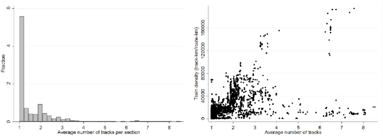
Table 5 lists variables for infrastructure characteristics, which describe technical aspects such as track length (includes parallel tracks) and route length, as well as the condition of the asset (rail age and switch age), and its capability (quality class and rail weight). Track length divided by route length gives us the average number of tracks on a section. This is an important variable for describing the available line capacity since 100 trains running on either one or two tracks during a given period will imply different levels of capacity utilisation. Still, we acknowledge that this is only a proxy for available line capacity (see also the introduction of section 2 regarding line capacity utilisation). A large share of the sections has around one track, as indicated by Figure 1a. Still, there is significant share of the observations that has more than one track, which is important for testing the hypothesis in this paper, stating that, for a given tonnage level, renewal costs vary with respect to line capacity utilisation. The traffic levels on these sections are shown in Figure 1b, indicating that there is a set of observations with traffic levels that stand out (above 110 000 trains per year). These may have a significant impact on the estimation results, despite comprising only 35 out of 3385 observations. We therefore consider an exclusion of these 35 observations in the model estimations (estimation results with these outliers are presented in the appendix).

(17)

15

Fig. 1a (left) Histogram of observations with respect to number of tracks. Fig. 1b. (right) Scatterplot

of train density against number of tracks.

Table 5. Descriptive statistics, data per section and year (3385 obs.)

Variables Median Mean Std. dev. Min Max

Characteristics

Route-km 38.11 50.92 41.08 1.89 219.39

Track-km 54.25 67.27 51.66 1.89 305.54

Average no. of tracks (track-km/route-km) 1.16 1.64 1.08 1.00 8.53 Switches, track-km 1.28 1.71 1.69 0 14.40

No. of stations 6 6.85 4.99 1 31

No. of joints 129 161 134 1 1221

Average age of switches 20.0 20.5 10.0 0 55.3

Average rail age 20.1 21.5 10.8 1 97.0

Station section, dummy variable 0 0.11 0.32 0 1

Capability and management

Average rail weight, kg/m 50.0 51.2 5.0 32 60 Quality class, 0 (high linespeed) to 5 (low linespeed) 2.2 2.2 0.2 0.0 5.0 West region, dummy variable 0 0.17 0.37 0 1 North region, dummy variable 0 0.13 0.33 0 1 Central region, dummy variable 0 0.18 0.39 0 1 South region, dummy variable 0 0.27 0.44 0 1 East region, dummy variable 0 0.25 0.43 0 1

Capability variables are important control variables in the model estimations. The reason is that higher traffic levels can be correlated with investments in capability, which are carried out to minimize long rung costs. Since track access charges should reflect SRMC, we need to purge the traffic estimates of

(18)

16 long run cost components. Quality class (determines maximum linespeed) and rail weight are the main capability variables.

We have information about the different regions each track section belongs to. These regions are considered to capture the impact of weather, management practices, and to some extent differences in wages where for example the West, South and East regions have larger cities, which is linked to higher wages. Moreover, a set of year dummy variables are included in the model estimations to control for year specific effects, such as overall changes in input prices or in budget constraints.

5. Results

Corners solution models are estimated for 1) all assets, 2) track, 3) electric installations, 4) signalling, and 5) telecommunication and other installations. The reason for combining telecommunication and other installations is that none (or few) of the components within these technical subsystems deteriorate due to traffic. Note, however, there can still be a marginal cost for traffic on these assets as described by Nilsson and Odolinski (2018). In short, an accelerated frequency of renewals when traffic increases is also motivated on technical subsystems with no traffic-related deterioration since the consequences of infrastructure failures will be larger.

We estimate Twopart models and Heckit models. Based on the EMSE of the traffic estimates, the Twopart model is preferred for Model 2 (track), Model 3 (electric installations), and Model 5 (telecommunication and other installations), whilst the Heckit model is preferred for Model 3 (signalling). The EMSE is more or less the same between Twopart and Heckit for Model 1 (all assets), where we choose the former. See Table 14 in the appendix.

Estimation results are presented in section 5.1, followed by section 5.2 with a presentation of the estimated marginal costs. The estimation results are based on 3350 observations (215 track sections), which means that 35 observations are excluded based on their significantly higher traffic levels (see Figure 2). The estimation results for Model 1 (all assets) that includes these 35 observations are presented in the appendix, which are not substantially different from results presented in Table 6, yet the traffic estimates are slightly different. We therefore prefer estimation results that exclude the 35 observations.

5.1 Estimation results

The average number of tracks and its interaction with train density is used to estimate the impact of line capacity utilisation, whilst holding deterioration effects constant. To test the impact of including these variables, we estimate Model 1a without these variables and then include them in Model 1b. The estimation results are presented in Table 6, showing the output from both the selection equation

(19)

17 (probability of renewal) and the outcome equation (renewal costs). Figure 3a and Figure 3b shows the cost elasticities with respect traffic, illustrating the impact of including average number of tracks and its interaction with train density.

The coefficient for the (average) number of tracks has the expected negative sign in both the selection and outcome equations, however, it is only statistically significant in the selection equation. The interaction term between number of tracks and train density is also negative in both equations, and statistically significant.

Cost elasticities with respect to traffic are calculated using eq. (5), i.e. estimates from the selection and outcome equation are combined. These are statistically significant at the one per cent level in Model 1a (0.688, standard error 0.132) and in Model 1b (0.776, standard error 0.138). See Table 14 in the appendix, which presents elasticities evaluated at the sample mean (average and median elasticities are presented in Table 11). The scatterplot of cost elasticities in Model 1a (see Figure 3a) indicates that the elasticity estimates increase with traffic, yet with no variation between different track intervals. The effect of the interaction term between train density and number of tracks is shown in Figure 3b. This is further illustrated in Figure 4a and Figure 4b, which are based on the same cost elasticities in Model 1b but using two separate track intervals in each figure. Specifically, comparing elasticities between different track intervals, whilst keeping the x-axis fixed (i.e. fixed train density), indicates that the line capacity utilisation (as measured by average train density per track on a section during a year) has an impact on renewal costs, even when controlling for deterioration effects. We therefore prefer model specifications that include variables for number of tracks and its interaction with train density (Model 1b and Model 2 to 5).

The average train weight may capture deterioration costs since track deterioration is to a large extent determined by axle loads. Indeed, the weight of the trains has a significant impact on renewal costs according to the estimation results. The cost elasticity is 0.772 (standard error 0.152) in Model 1a and 0.768 (standard error 0.151) in Model 1b.

Turning to the parameter estimates for the other variables in Model 1b, we can first note that track length and rail age are statistically significant and have the expected signs. This is also the case for the total track length of switches on each section, the number of stations, as well as whether the entire track section is a station or not. Quality class does not have a significant impact on the probability of a renewal (selection equation: p-value 0.106) but is positive and statistically significant in the outcome equation. Note that a higher quality classification number implies lower linespeeds.

(20)

18

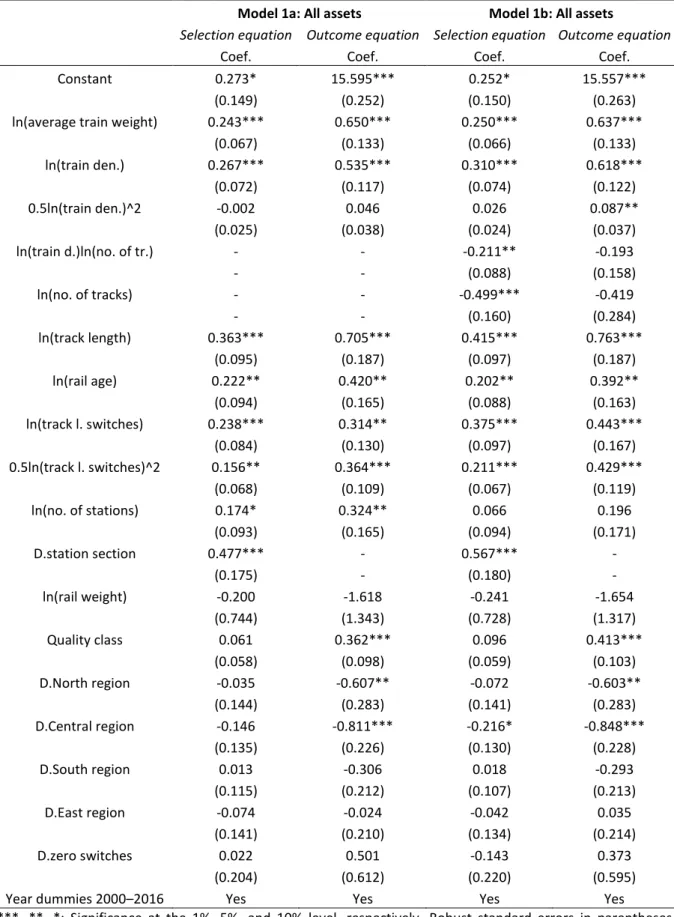
Table 6. Estimation results Model 1a and Model 1b, all assets (3350 obs.)

Model 1a: All assets Model 1b: All assets

Selection equation Outcome equation Selection equation Outcome equation

Coef. Coef. Coef. Coef.

Constant 0.239 15.555*** 0.219 15.541*** (0.148) (0.252) (0.148) (0.263) ln(average train weight) 0.244*** 0.639*** 0.251*** 0.630***

(0.067) (0.134) (0.066) (0.134) ln(train den.) 0.268*** 0.541*** 0.310*** 0.612*** (0.072) (0.115) (0.074) (0.119) 0.5ln(train den.)^2 -0.002 0.053 0.026 0.098*** (0.025) (0.037) (0.024) (0.037) ln(train d.)ln(no. of tr.) - - -0.220** -0.287* - - (0.095) (0.166) ln(no. of tracks) - - -0.492*** -0.451 - - (0.159) (0.282) ln(track length) 0.361*** 0.672*** 0.415*** 0.734*** (0.095) (0.187) (0.098) (0.185) ln(rail age) 0.224** 0.417** 0.204** 0.393** (0.095) (0.166) (0.087) (0.163) ln(track l. switches) 0.234*** 0.302** 0.361*** 0.418** (0.084) (0.132) (0.097) (0.166) 0.5ln(track l. switches)^2 0.159** 0.370*** 0.205*** 0.417*** (0.070) (0.120) (0.070) (0.123) ln(no. of stations) 0.176* 0.356** 0.064 0.221 (0.093) (0.164) (0.094) (0.170) D.station section 0.472*** - 0.565*** - (0.176) - (0.181) - ln(rail weight) -0.206 -1.598 -0.228 -1.608 (0.744) (1.345) (0.728) (1.319) Quality class 0.061 0.349*** 0.096 0.397*** (0.058) (0.099) (0.059) (0.103) D.North region -0.033 -0.575** -0.074 -0.592** (0.144) (0.282) (0.140) (0.284) D.Central region -0.145 -0.797*** -0.218* -0.855*** (0.135) (0.226) (0.130) (0.230) D.South region 0.014 -0.308 0.018 -0.295 (0.115) (0.211) (0.106) (0.213) D.East region -0.072 -0.008 -0.044 0.040 (0.141) (0.212) (0.133) (0.215) D.zero switches 0.034 0.521 -0.134 0.382 (0.203) (0.607) (0.218) (0.575) Year dummies 2000–2016 Yes Yes Yes Yes

***, **, *: Significance at the 1%, 5%, and 10% level, respectively. Robust standard errors in parentheses. Variables with interactions and second order effects have been divided by the sample mean prior to logarithmic transformation; thus, their first-order coefficients are effects at the sample mean.

(21)

19 A dummy variable for sections that only comprise a station is included in the selection equation and the parameter estimate show a significant effect. We also include a variable for the number of stations along the route of a section to control for density of (unobserved) components. However, the parameter estimates do not indicate a significant impact on renewals (this is also the case for Model 2 to Model 5).

Fig. 3a (left) Cost elasticities, all assets (Model 1a). Fig. 3b (right) Cost elasticities, all assets (Model 1b)

Fig. 4a (left) Cost elasticities, all assets (Model 1b: no. of tracks 1.00-1.74 and 2.50-3.49). Fig. 4b (right) Cost elasticities, all assets (Model 1b: no. of tracks 1.75-2.49 and 3.50-8.53).

Model 2 considers track renewals and the estimation results are presented in Table 7. The cost elasticities with respect to train density are statistically significant (0.748, standard error 0.150). Scatterplots of the cost elasticities in Model 2 are presented in Figure 5a and Figure 5b, indicating that capacity utilisation has an impact on track renewal costs, even when holding deterioration effects constant. Estimation results for model 2 also indicate that train weight can explain costs related to

(22)

20 track deterioration, yet there is no second order effect. The cost elasticity is statistically significant at the one per cent level (0.631, standard error 0.154). We can also note that most control variables, such as track length, rail age, total track length of switches, and quality class have similar effects as in Model 1. The number of joints did not have an impact on costs in Model 1 (and is excluded in the preferred model) but has a significant impact in Model 2.

Estimation results for electric installations (Model 3) are also presented in Table 7, showing that train density has a significant impact on renewal costs. Its interaction term with the number of tracks is negative, indicating that more trains on more tracks have a lower cost impact compared to the same amount of extra trains running on fewer tracks (in line with the hypothesis in the paper). A second order term for trains was tested but was not statistically significant.

It is not clear why the average weight of trains has a significant impact on renewal costs for electric installations, but one explanation could be that it is associated with enhancements in the electric installations and/or more components (such as feeding points) being required on lines with higher train weights. It may therefore be considered an important control variable for capability (i.e. avoiding long run cost components). Note also that rail weight is included in the model estimations, which is not directly related to the electric installations but considered to be a control variable for capability since heavier rails are usually installed on higher quality (and newer) lines. This is also the case for number of joints. Moreover, switches are included in Model 3 since a train moving from one track to another may have an impact on overhead wires compared, and indeed estimation results indicate a significant cost impact.

(23)

21

Table 7. Estimation results Model 2 (track) and Model 3 (electric installations) (3350 obs.)

Model 2: Track Model 3: Electric installations

Constant -0.189 14.867*** -0.465*** 14.394*** (0.146) (0.275) (0.171) (0.385) ln(average train weight) 0.181*** 0.477*** 0.440*** 0.638***

(0.069) (0.125) (0.090) (0.220) 0.5ln(ave. train weight)^2 - 0.190 - -

- (0.150) - - ln(train den.) 0.365*** 0.438*** 0.331*** 0.483*** (0.073) (0.124) (0.069) (0.172) 0.5ln(train den.)^2 0.033 0.114*** - - (0.029) (0.044) - - ln(train d.)ln(no. of tr.) -0.202*** -0.229 -0.212** -0.224 (0.077) (0.194) (0.097) (0.288) ln(no. of tracks) -0.204 -0.256 -0.440** -0.417 (0.157) (0.259) (0.187) (0.373) ln(track length) 0.464*** 0.482** 0.257** 1.065*** (0.106) (0.234) (0.120) (0.146) ln(rail age) 0.229*** 0.520*** - - (0.081) (0.182) - - ln(joints) 0.027 0.244*** -0.147** -0.415*** (0.061) (0.095) (0.071) (0.105) ln(track l. switches) 0.218** 0.352** 0.279** - (0.096) (0.139) (0.114) - 0.5ln(track l. switches)^2 0.202** 0.425*** 0.162** - (0.082) (0.122) (0.074) - ln(no. of stations) 0.021 0.252 0.113 - (0.101) (0.203) (0.122) - D.station section 0.111 - 0.388** - (0.163) - (0.191) - ln(rail weight) -0.694 -1.226 -0.822 -4.579*** (0.731) (1.373) (0.670) (1.557) Quality class 0.167*** 0.340*** 0.030 0.116 (0.057) (0.097) (0.071) (0.163) D.zero switches 0.404 1.263*** 0.076 - (0.325) (0.483) (0.449) -

Region dummies Yes Yes Yes Yes

Year dummies 2000–2016 Yes Yes Yes Yes

(24)

22

Fig. 5a. (left) Cost elasticities, tracks (Model 2: no. of tracks 1.00-1.74 and 2.50-3.49). Fig. 5b. (right) Cost elasticities, tracks (Model 2: no. of tracks 1.75-2.49 and 3.50-8.53).

Fig. 6a. (left) Cost elasticities, electric install. (Model 3: no. of tracks 1.00-1.74 and 2.50-3.49). Fig. 6b. (right) Cost elasticities, electric install. (Model 3: no. of tracks 1.75-2.49 and 3.50-8.53).

Estimation results for signalling renewals are presented in Table 8 together with results for renewal costs in telecommunication and other installations. As mentioned previously, based on the EMSE, the Heckit model is preferred for signalling, as opposed to the Twopart model which is preferred for the other asset types (Model 1, 2, 3, and 5).

Like Model 1 to Model 3, we include quality class in the Model 4 and Model 5 to control for capability and avoid long run cost components. Moreover, the number of stations, switches, and track length may be correlated with the number of signalling assets, telecommunication, and other assets, and are therefore also included in the model estimations. However, most explanatory variables are dropped in the outcome equation for signalling (Model 4) since their correlation with train density generate a negative coefficient for the latter. Still, region dummies and year dummies are included.

(25)

23

Table 8. Estimation results Model 4 (signalling) and Model 5 (tele. and other install.) (3350 obs.)

Model 4: Signalling Model 5: Telecom. and other install.

Constant -1.002*** 16.744*** -0.960*** 10.524*** (0.169) (0.954) (0.155) (0.478) ln(train den.) 0.182*** 0.008 0.306*** 0.387*** (0.061) (0.115) (0.057) (0.142) 0.5ln(train den.)^2 0.031 - - 0.260** (0.019) - - (0.125) ln(train d.)ln(no. of tr.) -0.284*** - -0.184* - (0.080) - (0.097) - ln(no. of tracks) -0.346** - -0.244 -0.906** (0.174) - (0.163) (0.391) ln(track length) 0.141 - 0.206** 0.212 (0.111) - (0.103) (0.166) ln(rail age) 0.153** - - - (0.067) - - - ln(joints) 0.040 - - - (0.052) - - - ln(track l. switches) 0.203** - 0.183** 0.401** (0.088) - (0.087) (0.177) 0.5ln(track l. switches)^2 0.111** - 0.108** 0.317** (0.057) - (0.055) (0.129) ln(no. of stations) 0.153 - 0.130 - (0.101) - (0.108) - D.station section 0.611*** - 0.225 - (0.211) - (0.191) - Quality class 0.125** - 0.031 0.045 (0.059) - (0.050) (0.107) D.zero switches -0.406 - -0.708** 1.460** (0.329) - (0.286) (0.611)

Region dummies Yes Yes Yes Yes

Year dummies 2000–2016 Yes Yes Yes Yes

Train density has a significant impact on the decision to renew signalling installations (selection equation), whilst the impact is close to zero for the expenditure decision (outcome equation). The number of tracks and its interaction with train density also have an impact in the selection equation, but this effect could not be found in the outcome equation. The scatterplots of the cost elasticities (Figure 7a and Figure 7b) indicate that there is no (clear) relationship between capacity utilisation and renewal costs in signalling installations. This is also the case for renewals in telecommunication and

(26)

24 other installations (Figure 8a and Figure 8b), yet the cost elasticities do increase with train density. Recall that cost increases due to increased line capacity utilisation (in addition to deterioration costs) could be explained by higher renewal frequencies – and/or more components being renewed – to curb expected increases in delay costs, and/or capacity utilisation affecting the cost of carrying out the project in terms of restrictions in production. The former explanation is more likely to be the case for signalling (Model 4), and telecommunication and other installations (Model 5) since there is no interaction effect between trains and number of tracks in the outcome equation, whilst this effect can be found in the selection equation. Overall, the signalling cost elasticity is statistically significant (0.278, standard error 0.145), which is also the case for telecommunication and other installations (0.855, standard error 0.178).

Fig. 7a. (left) Cost elasticities, signalling installations (Model 4c: tracks 1.00-1.74 and 2.50-3.49). Fig. 7b. (right) Cost elasticities, signalling installations (Model 4c: tracks 1.75-2.49 and 3.50-8.53).

Fig. 8a. (left) Cost elasticities, tele. and other install. (Model 5: tracks 1.00-1.74 and 2.50-3.49). Fig. 8b. (right) Cost elasticities, tele. and other install. (Model 5: tracks 1.75-2.49 and 3.50-8.53).

(27)

25

5.2 Marginal costs

We calculate marginal cost per train-km using cost elasticities with respect to train density and multiply by average costs. Equation (8) is then used to calculate weighted average marginal costs. Average costs, elasticities, and marginal costs for Models 1 to 5 are presented in Table 9. We also calculate weighted averages for the average costs and cost elasticities, using train-km as weights (like the weighted marginal cost calculation). There is a significant difference in average costs between the technical subsystems, whilst the cost elasticities are relatively similar (except for signalling which has the lowest elasticity). There are a few outliers in the marginal cost estimates, reflected by the difference between mean marginal costs and weighted average marginal costs (and the mean marginal cost for signalling is even negative due to outliers)

Table 9. Average costs, elasticities, and marginal costs: Model 1 to Model 5

Median Mean Weighted average

Average costs (per train-km), SEK

Model 1b: All assets 0.824 52.771 10.587

Model 2: Track 0.007 30.245 7.114

Model 3: Electric installations 0 2.270 1.781

Model 4: Signalling 0 18.573 0.812

Model 5: Telecom. and other installations 0 0.569 0.353

Cost elasticities

Model 2: Track 0.683 0.693 0.675

Model 3: Electric installations 1.036 1.038 0.862

Model 4: Signalling 0.299 0.296 0.259

Model 5: Telecom. and other installations 0.748 0.723 0.808

Marginal costs per train-km, SEK

Model 2: Track 0.004 3.574 4.434

Model 3: Electric installations 0 1.962 1.451

Model 4: Signalling 0 -1.357 0.134

Model 5: Telecom. and other installations 0 0.326 0.262

The weight of the trains has an impact on the deterioration of tracks. Model 1 and Model 2 take this effect into account by including a variable for the average train weight (Model 3 also includes a train weight variable but is not considered to capture the effect of increased deterioration caused by higher vertical forces). We use the estimated cost elasticities with respect to train weight to differentiate the weighted average marginal costs for all assets and tracks (see eq. 9). Results from a set of example calculations are presented in Table 10, where the sample mean (per year and per track section) at 528 tons and its corresponding costs (also in Table 9) are in bold text.

(28)

26

Table 10. Weighted average marginal costs differentiated using average train weight (eq. 9)

Train weight, gross tons Model 1b Model 2

200 3.915 2.697 400 6.093 3.756 528 (sample mean) 7.486 4.434 600 8.270 4.816 800 10.448 5.875 1000 12.625 6.935

To evaluate marginal cost variations with respect to line capacity utilisation, we calculate the weighted average marginal costs for two different train density intervals and two different track intervals, generating a 2*2 matrix. These marginal costs for all assets (Model 1b) and track (Model 2) are presented in Table 11, showing a pattern that is in line with the hypothesis in this paper: the highest marginal cost is found for observations with the highest train density interval combined with the lowest number of tracks, and vice versa. This is also illustrated in Figure 9 and in Figure 10, where each figure is based on the weighted average costs presented in Table 11 (thus generating plane surfaces, which is not the case if we consider each marginal cost observation).

However, the difference in costs between train density intervals (i.e. comparing columns in Table 11 and Table 12) may also include deterioration effects, even though we control for average train weight in the model estimations.

Table 11. Weighted average marginal cost, SEK per train-km, Model 1b and Model 2

Train density = [10K, 100k] Train density = [0, 10k]

Model 1b: All assets

No. of tracks = [1.00, 2.49] 11.168 3.948 No. of tracks = [2.50, 8.53] 7.456 1.490

Model 2: Track

(29)

27

Fig. 9. (left) Illustration of marginal costs in Table 11, all assets, Model 1b. Fig. 10. (right) Illustration of marginal costs in Table 11, track, Model 2.

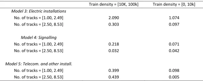
Weighted average marginal costs for electric installations, signalling, telecommunication and other installations are presented in Table 12. Most of these are line with the hypothesis in the paper. However, note that the cost elasticities for telecommunications and other installations indicate a weak relationship with line capacity utilisation (see section 5.1), which is reflected by the fact that the weighted average marginal cost is even higher for sections with a higher number of tracks, given a train density interval between 10 to 100 thousand trains per year.

Table 12. Weighted average marginal cost, SEK per train-km: Model 3, Model 4, and Model 5.

Train density = [10K, 100k] Train density = [0, 10k]

Model 3: Electric installations

Model 4: Signalling

Model 5: Telecom. and other install.

6. Conclusion

This paper contributes to the existing literature by demonstrating that increased capacity utilisation may – in addition to increased deterioration – generate increased costs for carrying out renewals and/or more frequent renewals. The econometric model estimations show that train density together with the average number of tracks can explain variations in marginal renewal costs, whilst controlling for average train weight, infrastructure characteristics and capability. Specifically, the renewal cost impact of an extra train is higher if it runs on sections with one track instead of two tracks – an effect

(30)

28 that has not been estimated in previous literature. This cost impact can be found for most of the technical subsystems that have been analysed in this paper, comprising track, electric installations, signalling, and telecommunication and other installations.

There are however differences in the estimates, where especially signalling and telecommunications and other installations stand out: results indicate that increased capacity utilisation will accelerate the renewal frequency on these assets, but it has no impact on the expenditure, i.e. costs for carrying out the project. This can be compared to track and electric installations where results indicate an impact on both the decision to renew (selection equation) and the expenditure decision (outcome equation). Our interpretation is that the effect of line capacity utilisation on the decision to renew is related to an IM trying to reduce the consequences of assets that fail (described in Nilsson and Odolinski, 2018), whilst its effect on the expenditure concerns the variation in production costs due to factors such as restrictions in renewal production (further described in section 2).

The results in this paper corroborates the results in Odolinski and Boysen (2019), where a similar analysis was carried out for maintenance cost of railways. Certainly, line capacity utilisation has an impact on marginal costs for infrastructure provision, and this impact is not only related to deterioration caused by traffic. This could be one explanation for why econometric results on renewal cost variability due to traffic are higher compared to results from engineering methods that focus on deterioration effects: see for example Smith and Nash (2018) for a discussion on econometric and engineering evidence using Great Britain as a case study.

Given that long run cost components (i.e. costs related to capability such as line speed) have been avoided in the estimations, the cost estimates can form a basis for track access charges as stipulated by the European Commission. Here it can be noted that this paper has used control variables for capability to exclude long run costs, however these variables are mainly concerned with track capability and not electric installations, signalling and telecommunications. Finally, it is important to note that this paper only considers the impact on production costs of the infrastructure services and should not be confounded with scarcity costs and congestion costs, which are also capacity related costs.

Acknowledgements

The authors are grateful to Trafikverket and the European Commission Horizon 2020 Shift2Rail project NEXTGEAR (grant number 881803) for funding this research. Special thanks to Gunilla Björklund for very helpful comments on an earlier version of this paper. All remaining errors are the responsibility of the authors.

(31)

29

References

Andersson, M., 2006. Marginal Cost Pricing of Railway Infrastructure Operation, Maintenance, and Renewal in Sweden - From Policy to Practice through Existing Data. Transportation Res. Rec. 1943, 1-11.

Andersson, M., Björklund, G., Haraldsson, M., 2016. Marginal railway track renewal costs: A survival data approach. Transportation Research Part A, 87, 68-77. DOI: https://doi.org/10.1016/j.tra.2016.02.009

Andersson, M., Smith, A., Wikberg, Å., Wheat, P., 2012. Estimating the marginal cost of railway track renewals using corner solution models. Transportation Research Part A, 46, 954-964. DOI: https://doi.org/10.1016/j.tra.2012.02.016

Attinà, M., Basilico, A., Botta, M., Brancatello, I., Gargani, F., et al, 2018. Assessment of unit costs (standard prices) of rail projects (CAPital EXpenditure). EU publications, final report contract 2017CE16BAT002. DOI: https://doi.org/10.2776/296711

Booz Allen Hamilton, TTCI. 2005. Review of Variable Usage and Electrification Asset Usage Charges: Final Report, Report R00736a15, London, June.

Dow, W.H., Norton, E.C., 2003. Choosing Between and Interpreting the Heckit and Two-Part Models for Corner Solutions. Health Services & Outcomes Research Methodology, 4, 5-18. DOI: https://doi.org/10.1023/A:1025827426320

Gradinariu, T., Kirwan, A, Gardin, D, et al, 2015. Key cost drivers in railway asset management. UIC Asset Management Working Group.

Hedström, R., 2020. Tider i spår för underhållsarbeten. (Track possession Time for Maintenance Work). VTI rapport 1043. (In Swedish).

Johansson, P., Nilsson, J-E., 2004. An economics analysis of track maintenance costs. Transport Policy, 11, 277-286. DOI: https://doi.org/10.1016/j.tranpol.2003.12.002

Leung, S. F., Yu, S., 1996. On the choice between sample selection and two-part models. Journal of Econometrics, 72(1-2), 197-229. DOI: https://doi.org/10.1016/0304-4076(94)01720-4

Lidén, T., Joborn, M., 2016. Dimensioning windows for railway infrastructure maintenance: Cost efficiency versus traffic impact. Journal of Rail Transport Planning and Management, 6, 32-47. DOI: https://doi.org/10.1016/j.jrtpm.2016.03.002

Lloyd’s Register Rail (2012). Possession management review. For PR13, for Office of Rail Regulation. Final Report, 16 July.

Marti, M., Neuenschwander, R., Walker, P., 2009. CATRIN (Cost Allocation of TRansport INfrastructure cost), Deliverable 8 – Rail Cost Allocation for Europe – Annex 1B – Track maintenance and renewal costs in Switzerland. VTI, Stockholm.

(32)

30 Nash, 2018. Track access charges: reconciling conflicting objectives Project report. 9 May. CERRE,

Centre on Regulation in Europe.

Nilsson, J-E., Nyström, J., Salomonsson, J., 2019. Kostnadsöverskridande i Trafikverkets entreprenadkontrakt. (Cost overruns in construction contracts tendered by the Swedish Transport Administration) VTI rapport 1011. (In Swedish).

Nilsson, J-E., Odolinski, K., 2018. Marginalkostnader för reinvesteringar i olika järnvägsanläggningar: En delrapport inom SAMKOST 3. CTS Working paper 2018:22. Centre for Transport Studies, Stockholm. (In Swedish)

Odolinski, K., Boysen, H.E., 2019. Railway line capacity utilisation and its impact on maintenance costs. Journal of Rail Transport Planning & Management, 9, 22-33. DOI: https://doi.org/10.1016/j.jrtpm.2018.12.001

Odolinski, K., Wheat, P., 2018. Dynamics in rail infrastructure provision: Maintenance and renewal costs in Sweden, Economics of Transportation, 14, 21-30. DOI: https://doi.org/10.1016/j.ecotra.2018.01.001

Smith, A.S.J., 2008. International Benchmarking of Network Rail’s Maintenance and Renewal Costs: An Econometric Study Based on the LICB Dataset (1996–2006). Report for the Office of Rail Regulation, Report Written as Part of PR2008, October 2008.

Smith, A.S.J., Iwnicki, S., Kaushal, A., Odolinski, K., Wheat, P., 2017. Estimating the relative cost of track damage mechanisms: combining economic and engineering approaches. Proceedings of the Institution of Mechanical Engineers, Part F: Journal of Rail and Rapid Transit, 231(5), 620-636. DOI: https://doi.org/10.1177/0954409717698850

Smith, A.S.J., Nash, C., 2018. Track access charges: reconciling conflicting objectives Case Study – Great Britain. 9 May. CERRE, Centre on Regulation in Europe.

Smith, A.S.J., Odolinski, K., Hossein-Nia, S., Jönsson, P-A., Stichel, S., Iwnicki, S., Wheat, P., Estimating the marginal maintenance cost of different vehicle types on rail infrastructure. Proceedings of the Institution of Mechanical Engineers, Part F: Journal of Rail and Rapid Transit. (Forthcoming) Tervonen, J., Pekkarinen, S., 2007. Marginal rail infrastructure costs in Finland 1997–2005. Publication

of the Finnish Rail Administration, A 3/2007.

UIC, 2013. UIC Code 406, Capacity, second ed. Original, UIC, International Union of Railways June 2013. Öberg, J., Andersson, E., Gunnarsson, J., 2007. Track Access Charging with Respect to Vehicle