Fault detection of planetary gearboxes in BLDC-motors using vibration and acoustic noise analysis

(1)

UPTEC E 20026

Examensarbete 30 hp

November 2020

Fault detection of planetary

gearboxes in BLDC-motors using

vibration and acoustic noise analysis

(2)

Teknisk- naturvetenskaplig fakultet UTH-enheten Besöksadress: Ångströmlaboratoriet Lägerhyddsvägen 1 Hus 4, Plan 0 Postadress: Box 536 751 21 Uppsala Telefon: 018 – 471 30 03 Telefax: 018 – 471 30 00 Hemsida: http://www.teknat.uu.se/student

Abstract

Fault detection of planetary gearboxes in

BLDC-motors using vibration and acoustic noise

analysis

Henrik Ahnesjö

This thesis aims to use vibration and acoustic noise analysis to help a production line of a certain motor type to ensure good quality. Noise from the gearbox is sometimes present and the way it is detected is with a human listening to it. This type of error detection is subjective, and it is possible for human error to be present. Therefore, an automatic test that pass or fail the produced Brush Less Direct Current (BLDC)-motors is wanted. Two measurement setups were used. One was based on an accelerometer which was used for vibration measurements, and the other based on a microphone for acoustic sound measurements. The acquisition and analysis of the measurements were implemented using the data acquisition device, compactDAQ NI 9171, and the graphical programming software, NI LabVIEW.

Two methods, i.e., power spectrum analysis and machine learning, were used for the analyzing of vibration and acoustic signals, and identifying faults in the gearbox. The first method based on the Fast Fourier transform (FFT) was used to the recorded sound from the BLDC-motor with the integrated planetary gearbox to identify the peaks of the sound signals. The source of the acoustic sound is from a faulty planet gear, in which a flank of a tooth had an indentation. Which could be measured and analyzed. It sounded like noise, which can be used as the indications of faults in gears. The second method was based on the BLDC-motors vibration characteristics and uses supervised machine learning to separate healthy motors from the faulty ones. Support Vector Machine (SVM) is the suggested machine learning algorithm and 23 different

features are used. The best performing model was a Coarse Gaussian SVM, with an overall accuracy of 92.25 % on the validation data.

ISSN: 1654-7616, UPTEC E 20026 Examinator: Mikael Bergkvist Ämnesgranskare: Ping Wu Handledare: Mats Freding

(3)

Popul¨

arvetenskaplig sammanfattning

M˚anga ljudanalyser sker i dagsläget via en operatör som lyssnar efter missljud. Vid produktion av servomotorer kan det uppst˚a defekter som kan detekteras via ljud/vibrations analyser. P˚a grund av subjektiv bedömning fr˚an operatör kan det leda till att felaktiga enheter g˚ar ut till kunder och även godkända enheter skrotas i onödan. Detta leder till onödiga kostnader. Servomotorernas defekter kan orsakas av material- eller monteringsfel, skadorna kan leda till förkortad livslängd/prestanda. Dessa defekter ger ofta upphov till missljud eller vibrationer. Arbetet utfördes p˚a Allied Motions kontor i Bromma. Arbetet best˚ar till en början av en litter-aturstudie kring vilka metoder det finns kring ljud/vibrations analyser. Senare undersöktes det vilka alternativ av automatisk test som finns för att identifiera servomotorer som har defekter. Stort fokus l˚ag p˚a metodutveckling för att hitta produktions defekter och missljud med hjälp av ljud/vibration analys. Datan som samlades in skedde med hjälp av mikrofon och accelerometer. Det var även av intresse att ta reda p˚a vad grundorsaken till defekter i servomotorerna är. Fyra föreslagna metoder testades, där tv˚a av dem visades sig framg˚angsrika. En metod baserade sig p˚a att spela in det missljud som kom fr˚an servomotorerna och sedan multiplicera singal med sig själv, därefter göra en Fast Fourier transform (FFT) och p˚a s˚a sätt indentifiera frekvensen p˚a missljudet. Denna frekvens hade en mattematisk koppling till planethjulet i växell˚adan och kunde p˚a s˚a sätt identifera vad grundorsaken till var defekten ligger i servomotorn. Den andra metoded baserade sig p˚a vägledd maskininlärning som tog sitt data fr˚an vibrationerna fr˚an ser-vomotorerna. Maskininlärning användes för att kunna göra avikelse detekering, vilket betyder att man kan gruppera in de servomotorer som saknar missljud och jämnföra med servomotoroer som har missljud. Grund algoritmen för maskininlärningen var Support Vector Machine (SVM) och den kunde bygga upp en dator modell med hjälp av tjugitre olika ”features”. Den slut-giltiga modellen blev en Coarse Guassian SVM som hade en övergriplig precission p˚a 92.25% för att kunna skilja defekta mot icke-defekta servomotorer.

(4)

Acknowledgments

I would like to thank my supervisors Erik Olsen and Mats Freding at AlliedMotion for giving me the opportunity to do my master thesis. A special thanks to Ali Algoz for the daily car-rides and the positive energy from Arash Zeinali.

I would also like to thank my project subject reader Ping Wu for the helpful comments on the report. Lastly a huge thanks to my family and friends who have supported me along the way. Tack s˚a mycket.

(5)

Glossary

Spectral analysis is a term used for analyzing the spectrum of frequencies. Inverter converts direct current to alternating current.

H-bridge is part of the inverter, four transistors placed looking like an H. Anomaly is something that deviates from what is normal.

Harmonics is used to describe the distortion of a sinusoidal waveform. Pinion is a round gear.

Gearbox is a mechanical system that transfer mechanical power from a rotating machine. It can be used to increase the torque output but lowering the output speed or vice versa depending on the transmission ratio.

(8)

Acronyms

AC Alternating Current AE Acoustic Emission

BLDC Brush Less Direct Current CCW Counter-clock Wise

CM Condition Monitoring CW Clock Wise

DC Direct Current

FFT Fast Fourier Transform FT Fourier Transform GMF Gearmesh Frequency

ISO International Organization for Standardization NVH Noise Vibration Harshness

PM Permanent Magnet PWM Pulse-width modulation RPM Revolutions Per Minute SVM Support Vector Machine

(9)

1 Introduction

Rotating machines generate sounds. The sounds from a machine operating in the condition without any defects differ from the one with defects, for example a cracked tooth in a gear. Therefore, the sounds that can be identified coming from defects can be exploited as the indica-tions of the defects. Monitoring the condiindica-tions in machinery such as sound, vibration, temper-ature is called condition monitoring (CM). CM can be implemented using different techniques. This master thesis focuses mainly on the CM technique, vibration and acoustic noise analysis. Sufficient knowledge about sounds and acoustic noise from rotating machinery is necessary for understanding the technique.

1.1 Background

When looking for noise present in smaller electrical motors it is common that there is a human ear behind the analysis. The human ear is amazing in many ways, however this analysis method leaves room for inconsistencies, since it is subjective. Therefore, a sound/vibration analysis with more consistent methods is preferred. With a more consistent analysis method, it could also increase the knowledge behind what is creating the noise. Noise and vibration analysis are common in larger factories, where they are used as fault analysis in order to prevent machinery failure. Are these sound/vibration analysis methods that are developed for larger machinery, applicable to smaller scale machinery?

1.2 Purpose and goals

The thesis aims to help a production line of a certain motor type to ensure good quality and help other designs of BLDC-motors to reduce their overall noise level. Moreover, unwanted noise from the gearbox is sometimes present and the way it is detected is by listening to it with a human ear. This type of error detection is subjective, and it is possible for human error to be present. Therefore, an automatic test that pass or fail the produced BLDC-motors with the help of a computer is wanted.

The goals of the thesis can be summarized as:

• Identify what causes the defect noise to be present in some of the newly produced BLDC-motors with integrated gearbox and drive.

• Investigate different techniques for an automatic test that can indicate if an motor is healthy or faulty according to its vibration/sound characteristics.

• Can this automatic vibration/sound test be implemented for quality assurance in a pro-duction line?

• With the knowledge gained from the investigation part of the thesis, is it possible to pin-point specific parts of an electric motor that can be changed in order to reduce overall noise?

(10)

1.3 Tasks and scope

The main scope of the thesis is to do a fault detection of gearboxes in BLDC-motors using vibration and acoustic noise analysis. The system that will do the fault analysis is based on vibration and sound data. Tasks that needs to be done to record reliable data are:

• Create a measurement setup for the vibration and the sound data. The setup includes the usage of a accelerometer and a microphone.

• Get familiar with LabVIEW and configure the tools needed to record data. • Choose appropriate sampling frequency and number of samples.

• Evaluate the need of filters.

The next step is to analyse the data using appropriate software (MATLAB and LabVIEW). The steps includes:

• Preform signal analysis in LabVIEW.

• Create plots of the recorded data using MATLAB.

• Use MATLAB to apply machine learning algorithms on the recorded data.

1.4 Outline

Chapter 1 presents the introduction of the thesis, which contains background, the purpose, the tasks and scope. Chapter 2 contains a technical background, which provides relevant background information about vibration principles and electrical motors. Chapter 3 present the relevant theory used, which covers the two main methods, signal analysis and machine learning. Chapter 4 present the four methods used for noise/vibration detection. Chapter 5 provides background information about different transducers and the measurement setup. Chapter 6 presents the results and the discussion of the vibration and acoustic noise analysis. Finally, a conclusion from the results and future work recommendation is presented in chapter 7.

(11)

2 Technical Background

2.1 Vibration/noise principles

Vibration analysis is one common method for fault analysis. Therefore it is important to know the theory behind vibrations. In short vibrations can be defined as back and forth motion of a system around it is equilibrium position. This chapter is to introduce the concepts about vibrations and how it can be measured. Two of the main relevant concepts are Noise, Vibration, Harshness (NVH) and Condition Monitoring (CM). [1] [2]

2.2 Noise, Vibration and Harshness (NVH)

The field of NVH theory is applied in the automobile engineering industry to give an analysis of where the source of noise and vibrations is and in terms of feeling and hearing. These terms are not subjective which means that some analysis made can be rather tricky since there might not be an absolute truth. Some noise is perceived more unpleasant than other to the human ear but there are no clear definitions for it. Even though NVH is a complex subject the sources can be divided into three parts:

1. Aerodynamic (Not a focus in this thesis) 2. Mechanical

3. Electrical

For an electrical motor with an integrated gearbox the two sources of NVH are mechanical and electrical. Aerodynamics is more important for analysing NVH in a car affected by e.g. the air resistance at higher speeds. The terminology related to the subject of NVH is listed below:

• Noise is unexpected or unwanted sound created by vibration in a machine. • Vibration is a repetitive back-and-forth/up-and-down motion of a body.

• Harshness can generally be described as the level of discomfort the noise from the machine is creating.

NVH related problems are usually of the repetitive nature, so a terminology for frequency is also included:

• Frequency is the number of completed cycles in each time frame.

• Order is defined as the number of events per revolution. A machine with rotating parts emits a response for each rotating part. Order is the way of identifying each rotating part to a certain frequency.

• Resonance is a way of describing the increase in amplitude that can be observed when a system is equal to its natural frequency.

(12)

2.3 Condition monitoring

The concept of detecting anomalies from the machine’s normal condition is called condition monitoring (CM). The main objective for CM is to asses the overall health of the machine. Fault diagnosis provides information of what caused the deviation from normal condition, may it be a component failure or a process that caused the anomaly. With the market’s demand of greater reliability and digital controller system becoming cheaper, this allows for a vast increase in CM applications.

There are several signal analysis techniques developed for CM, spectral analysis among other. Due to the repetitive nature of machines, mostly rotating machinery, spectral analysis is often applicable. Because defects are often detectable as changes in the spectrum of a measured signal. Usually the signals spectral characteristics can be associated with a physical feature such as the rotating speed of a shaft.

Every machine has its own unique baseline signature values, in terms of varying parameters, such as acoustic emission (AE), analysis of in-service lubrication and vibration spectral features. The challenge is then to detect deviant behaviour with help of all these different parameters. With modern technology it is possible to combine all this data from the machine, in order to asses its state. It is important to recognise early stage faults so that the damage can be minimized. In large complex system a faulty subsystem can shut down the whole system, if not repaired in time. However, it is not common practice to apply CM on small systems because it is often cheaper and easier to go with the run until failure approach. The recommended level of allowed vibration based on ISO 10816-1 only cowers the range 15-75 kW, which makes machines smaller than 15 kW to have less guidelines on how they should operate.

2.4 BLDC motor

The motor that is analysed in this thesis is a brush less direct current motor (BLDC) with connected planetary gearbox and inverter from AlliedMotion. A BLDC motor is a typical 3-phase synchronous electrical motor that requires an inverter/PWM drive to function, due to the inverter converting DC to AC so that the motor can rotate. The main parts in a electrical motor from AlliedMotion are the rotor, stator, PWM drive and a two stage planetary gearbox. Each one of these components is a source of vibration/acoustic sound. In theory, if each source gives out a unique frequency of vibration it should be possible to detect these vibrations and with this knowledge to detect any anomalies if a vibration frequency is higher than expected. 2.4.1 Rotor and stator

The rotor is the rotating part of the motor, which usually consists of several permanent magnets (PMs). The minimum requirement is 2 poles, one north and one south, but the rotor can have more than one pole pair. The stator is the stationary part of the motor and it usually consists of laminated iron plates which the coils can be winded through. If the coils are winded correctly, achieving symmetry, a three-phase system can be established, as shown in Figure 2.1.

(13)

Figure 2.1: A typical BLDC motor in which the rotor in the middle is surrounded by the stator.[3]

The most common sources of mechanical noise from an electric motor are [4]: • Angular or parallel misalignment of the rotor

• Unbalanced rotor

• Looseness between the laminated plate stack • Bearing related issues

These sources should have a frequency related to their rotation speed and other factors, more about this is presented in 3.2. With the known frequency of interest, it should be possible to know or see an indication of which part causes the noise. There could also be built in noise from the design of the motor which is not necessarily a fault but a cause of noise. Figure 2.2 gives some examples of common sources for design faults.

(14)

Figure 2.2: Common sources of acoustic noise from an electrical motor.[4]

2.4.2 PWM drive

The PWM drive is the controller part of the motor, converting DC to AC with the help of an H-bridge. This part usually contributes to high frequency noise, due to the high switching frequency.

(15)

2.4.3 Planetary gearbox

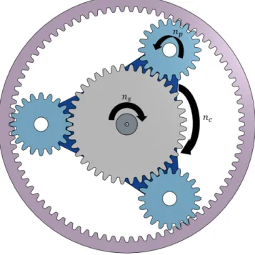
The gearbox mounted on an electrical motor is used to increase the output torque but in trade-off gets a lower output rotation per minute (RPM). The gearbox type in this thesis is a planetary/epicyclic gearbox with two stages, see Figure 2.4. The planetary gearbox consists of one ring gear with a fixed position, two or more planet gears, one planet carrier and one sun gear for each stage. Figure 2.5 is illustrating a single stage of a planetary gearbox, two stages means that there is another stage connected to the planet carrier, increasing the gear ratio in the gearbox. A planet gearbox can consist of several stages, where each gear has specific set of teeth and is often referred to as z and the rotational speed of a gear as n.

Figure 2.4: A two stage planetary gearbox.

(16)

3 Theory

3.1 Signal analysis and anomaly detection

This chapter provides a general introduction to two different methods that are needed for this thesis.

3.1.1 Fourier Transform and FFT

The Fourier transform (FT) is a way of transforming a signal in time domain to frequency domain. This transform is one of the most important mathematical tools available for extracting basic information from a signal. The FT for a signal x(t) is given by:

XT(ω) = Z ∞

−∞

x(t)e−jωtdt (3.1)

The power spectrum density (or simply power spectrum) of is given by: P (f ) = lim

T →∞ 1

T|XT(ω)|

2 _(3.2)

where XT(ω) is the Fourier transform of x(t) over a period of T.

An efficient algorithm of the FT is the fast Fourier transform (FFT) that is specifically used in this thesis to transform the vibration/sound time domain data into frequency domain. A more in-depth explanation on how it works can be found here [5].

3.1.2 Anomaly detection

Analysing vibration/sound data is required in this thesis. Some of these data observations have a larger difference than the majority data. These data observations are called anomalies or outliers. The broad field of anomaly detection is generally to detect anomalies/outliers in datasets. Anomaly detection is often part of machine- and/or statistical learning. There are several applications for anomaly detection since abnormal data is often a sign of something. Abnormal vibrations from a gearbox may indicate that the gearbox is defect. There are some general problems that need to be addressed when applying anomaly detection, such as:

• What should the difference between normal and abnormal data be? A line between these two needs to be decided. Drawing the line so that more data gets classified normal will result in a high false negative rate, which means missing anomalies. On the contrary, drawing the line so that more data gets classified abnormal results in high false alarm rate.

• Does the definition of abnormal and normal data change over time?

• It is almost impossible to have data that is not affected by noise, sometimes it can be hard to distinguish anomalies from noise, since it might have similar characteristics.

(17)

When applying anomaly detection, it is important to know what kind of data you are dealing with, so that the right method can be chosen and used. There are three main kinds of anomalies. [6]

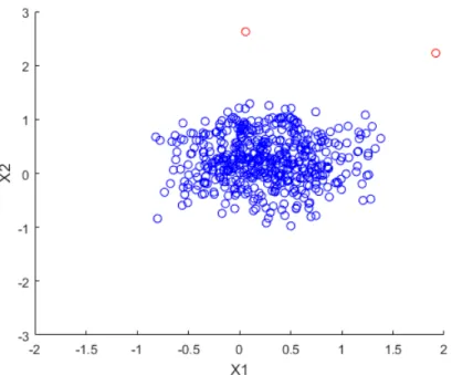
• Point anomalies, individual point that differs from the rest of the data, does not consider what the context could be, as shown in 3.6.

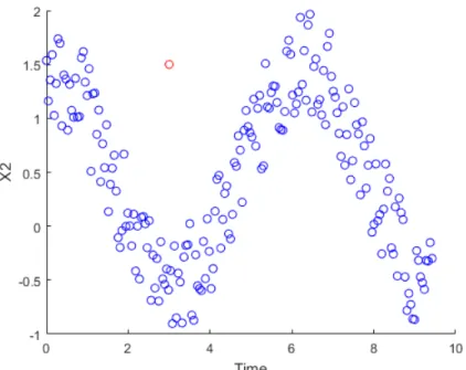
• Contextual anomalies, usually not a point anomaly in itself, but when taking context into account, it becomes an anomaly. For example, the weather in Sweden is 20 degrees, which could be normal or abnormal depending on the context. Were context is what time of the year the data was collected, as shown in 3.7.

• Collective anomalies, the individual data points might not be an anomaly but when forming a group with other data points it can be considered as an anomaly, as shown in 3.8.

Figure 3.6: Example of point anomalies. Variables X1 plotted against X2, forming a cluster. The anomalies are marked as red.

(18)

Figure 3.7: Example of context anomalies. The anomaly marked as red.

(19)

3.2 Theoretical frequencies of interest

With help of the FFT, a spectrum of frequencies will be available for analysis. Some frequencies are useful and of special interest for the gear’s conditions. Fault indications frequencies that are higher than normal or with increasing harmonics it can be seen as an indication of a fault etc.

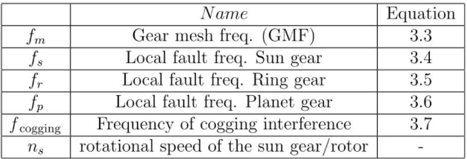
N ame Equation

fm Gear mesh freq. (GMF) 3.3

fs Local fault freq. Sun gear 3.4 fr Local fault freq. Ring gear 3.5 fp Local fault freq. Planet gear 3.6 fcogging Frequency of cogging interference 3.7 ns rotational speed of the sun gear/rotor

-Table 3.1: List of the frequencies of interest with reference to each equation.

The fault frequencies for the rolling element bearing is not included in this thesis. This is done to simplify the problem, with less frequencies of interest the easier the analysis of the FFT spectrum will be. However, this will also leave the possibility of unknown faults in the system to be present.

3.2.1 Planetary gearbox

When analyzing the state of the gearbox, gear mesh frequency (GMF) is a central part of the analysis. GMF should appear on the frequency spectrum regardless of condition, it tells the characteristics of each gear assembly. The variation of amplitude in the GMF and it’s harmonics could then be an indication of what the condition of the gearbox is. In short, the GMF analysis can be summarized as observing how a healthy gearbox looks in the frequency spectrum and then compare it to a faulty one with focus on the GMF and its harmonics. If Figure 2.5 is one stage of a planetary-gear, one relative revolution in the planet gear will have the same number of meshing teeth with the sun and ring gear. This means that the meshing frequency of planet to sun gear is the same as planet to ring gear. With a known rotation speed of the sun gear the gear mesh frequency for a single stage is then according to [7]:

fm = zrzs zr+ zs

ns (3.3)

Where zr is the number of teeth on the ring gear, zs is the number of teeth on the sun gear and ns is the rotational frequency of the sun gear. It is not only the specific GMF frequency that is interesting, the side-bands of the GMF are also of interest. Side-bands are the The rotating frequency of the pinion and the gear correspond to these side-bands. Which can be used as an indication to see if the gear or the pinion are in poor condition depending on the difference between the amplitude of a healthy and a faulty gear.

(20)

To find the local fault frequency in one of the gears, one can simply divide the gear mesh frequency by the number of teeth that the gears of interest have. See Figure 3.9.

Figure 3.9: A local fault in one gear tooth. 3.2.2 Local fault frequency of the sun gear

Applying this for a sun gear with a local fault such as Figure 3.9 and when considering that the sun gear meshes with the planet gears with a multiple of K gives according to eq. (3.3):

fs = K ∗fm zs

(3.4) Where fm is the gear mesh frequency, zs is the number of teeth on the sun gear and K is the number of planet gears. However, there is not certain that the amplitude will be the same for each mesh between the faulty sun tooth and the planet tooth. Since each gear gets slightly unique characteristics in the manufacturing process, this is important to keep in mind when looking at the local fault frequency for a sun gear. [7]

3.2.3 Local fault frequency of the ring gear

Similarly, as the case with the sun gear the expression for the local fault frequency of a ring gear can be derived as:

fr = K ∗ fm

zr

(3.5) Where fm is the gear mesh frequency, zr is the number of teeth on the ring gear and K is the number of planet gears.

3.2.4 Local fault frequency of the planet gear

The local fault frequency for a planet gear can be derived without considering how many planet gears that are present in the gearbox, since the planet gear only meshes with the sun and ring gear. Therefore, the local fault frequency can be derived as:

fp = fm

zp

(3.6) Where fm is the gear mesh frequency and zp is the number of teeth on the planet gear.

(21)

3.2.5 Switching frequency and harmonics of the PWM Drive

The most dominant source of vibration/acoustic noise from the PWM drive that is expected to be see is the switching frequency the power transistors operate at. The switching frequency is how often a transistor is turned ON and OFF during one period. However, several harmonics from the switching frequency will also be present and oscillation from the stray inductance, capacitance and the gate resistance will also contribute to the noise spectrum. The general experience from these kinds of circuit will give an expected frequency spectrum around 10-40 kHz.

3.2.6 Interference frequency in the BLDC electric motor

One of the possible main sources of vibration is from the rotor, since it is the rotating part. The frequency of the rotational speed of the rotor/sun gear, ns, is to be expected. However, the cogging torque is also a factor that needs to be considered, since it can be a source of vibration. The interference frequency due to cogging torque can be derived by calculating how many ”coggs” there are per revolution and then multiply it with the rotational speed of the sun gear: fcogging= 1 1 P − 1 Z ∗ ns (3.7)

Where P is the number of poles in the rotor, Z is the number of slots in the stator and ns is the rotational speed of the rotor.

3.3 Machine Learning

3.3.1 Introduction

There are three main types of anomaly detection methods, supervised, unsupervised and semi-supervised learning. These are general methods that are applicable for machine learning. Ma-chine learning is when a computer algorithm builds a mathematical model based on sample data, which is called training. This trained mathematical model can then make a prediction on new data. The different machine learning algorithms can be categorized as follows:

• Supervised machine learning means that the algorithms take previous known infor-mation, in the form of labelled/classified data, and apply it to new data to predict future events.

• Unsupervised machine learning is the opposite of supervised, which means the sam-pled data cannot be classified or labelled. The prediction from an unsupervised algorithm can be used to describe hidden structures from unlabelled data.

• Semi-supervised machine learning is the combination of supervised and unsupervised machine learning, so there will be some labelled- and unlabelled data available for training. This sort of learning is often used when the acquiring extra unlabelled data do not require extra resources. A rule of thumb in machine learning is that the model often will perform

(22)

better with a larger sample size. Since more data often include a wider possibility range which correlates to a more robust model.

To get a sense of what the difference between labelled and unlabelled data means, a simple example can be used. Imagine having a task to get a computer see the difference between photos of cats and dogs, representing two categories in this case. If there is prior information about the photos, meaning that a photo can either be labelled a cat or a dog. Then supervised machine learning can be applied and when shown a new photo the algorithm can make a prediction if that photo shows a cat or a dog. If there is no prior information known about the photos, unsupervised learning is applied. The algorithm will then go through all photos and sort them out into two categories, based on their properties. In this thesis there will be prior information about the collected data, therefore, supervised machine learning is the suggested method. No further explanation on the other methods is described in this thesis.

3.3.2 Supervised machine learning

As mentioned earlier, the dataset is labelled in supervised learning. This allows supervised learning to utilize labelled training data, so that it can learn to categorize data. If the training data is expressed as every element in the input data, vector x, then it requires an associated response measurement y, which is the label. The training data also needs to consist of both normal and anomaly categorized data. The input data, vector x, consists of features which are an individual measurable characteristics of an observation. The response, y, can either be of quantitative or qualitative nature. This is called regression or classification problems, respectively. Where the quantitative variable has a numerical value and the qualitative variable describe something, e.g. dog or cat. Quantitative outputs are defined as regression problems and qualitative outputs defined as classification problems. Anomaly detection is a typical classification problem, since it has a ’normal’ and a ’anomaly’ class. After the algorithm is trained based on the training data it can be used to categorize new data.

Supervised machine learning requires labelled data from both regions of the classes in order to be effective. A common problem in anomaly detection is that the ratio between normal and abnormal data is not evenly distributed. Which algorithm to choose for training is also not a ”strict” theory, since there is no way of knowing in advance which the best performing algorithm is. One example of a machine learning algorithm is Support Vector Machine (SVM) and these articles suggest that it can be used for fault detection in gearboxes [8][9][10][11]. Therefore, no other algorithm is described in this thesis.

(23)

3.3.3 Support Vector Machine

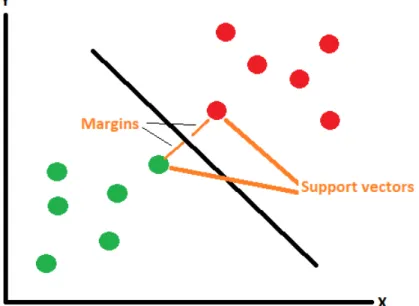
Support vector machine is a supervised machine learning algorithm which base idea is to find an optimal hyperplane that divides the labelled dataset into two classes, see Figure [12]. A hyperplane can be seen as a line that linearly separates the data. The equation for a p-dimensional hyperplane, H is given by:

H = β0+ β1X1+ β2X2+ · · · + βpXp = 0 (3.8) Where β is the defining parameter of the hyperplane and X is the data.

Figure 3.10: Example of a hyperplane that divides two classes from each other.

The datapoints closest to the hyperplane is called support vectors and are the critical elements in creating a dividing hyperplane. The distance between the hyperplane and the closest datapoint gives the margins. The preferred hyperplane is the one with the largest possible margin between any point of the training set. This gives a greater chance of new data being classified correctly. However, datapoints are often not as easily separated with a hyperplane as in this example. For non-linear datasets, meaning there is no clear visually separately hyperplane between the two datasets, a trick kerneling is used. Kerneling is basically a way of mapping data into a higher dimension, which then could make it possible to create a hyperplane segregating the classes. This is only a brief introduction, a more detailed explanation about how the SVM algorithm works and how it uses the kernel trick to classify non-linear data can be seen here [12].

(24)

3.3.4 Suggested Features

The input data for the machine to interpret, consists of features which are an individual mea-surable characteristics of an observation. It can be hard to know beforehand which features are suitable for machine learning, so it is often preferred to include several features when building a model. The features that is suggested for the SVM model to use for training are:

Root mean square (RMS) Standard deviation (SD) Mean absolute deviation (MAD)

Skewness Kurtosis Signal entropy Spectral entropy Maximum frequency Max ratio 25-Quantile 75-Quantile Interquartile range (iqr) Mel-frequency cepstral coefficients:

MFCCs 1 to 10 Table 3.2: List of the different features

The set of data can be described as (x1, x2, · · · , xn), where n is the number of data points. Root mean square is derived as:

xrms = r 1 n(x 2 1+ x22+ · · · + x2n) (3.9) Mean absolute deviation is the average of the absolute deviations from the mean of the data, MAD is derived as:

xmad= 1 n( n X i=1 xi− m(X)) (3.10)

Where m(X) is the mean value of the data set. Skewness is derived as:

¯ xskew= ( Pn i=1((xi− m(X)) 3_)/n) s(X)3 (3.11)

Where s(X) is the standard deviation and m(X) is the mean value of the data set. Kurtosis is derived as:

¯ xkurt = ( Pn i=1((xi− m(X)) 4_)/n) s(X)4 (3.12)

Where s(X) is the standard deviation and m(X) is the mean value of the data set.

Signal entropy is the estimate of the entropy of a stationary signal. It is a two-step process and the steps are:

(25)

• A histogram of the signal is estimated • From which the entropy can be calculated

A more in-depth explanation on the calculation of the signal entropy can be found here [13]. Spectral entropy is a measure of the signal’s spectral power distribution and is defined as:

P (m) = |F (X)| 2 P

i|F (X)|2

(3.13) Where P (m) is the probability distribution and F (X) is the discrete Fourier transform of the data set. The normalized spectral entropy Hn is then:

Hn = PN

m=1P (m)log2(P (m))

log2(N ) (3.14)

The definition of the maximum frequency is where the max of the power spectrum of the signal occurs in Hz, with respect to the cut-off frequency. The max ratio is defined as the ratio of the energy from the maximum frequency and the total energy from the spectrum, with respect to the cut-off frequency.

The quantile function can be defined as:

Q(p) = inf {x ∈ R : p ≤ F (x)} (3.15)

Where the probability has an interval of 0 < p < 1. 25-Quantile means that p = 0.25 and 75-Quantile means that p = 0.75.

Interquartile range (iqr) is the difference between the 25- and 75-Quantile, which can be defined as:

xiqr = Q(0.75) − Q(0.25) (3.16)

The Mel-frequency cepstral coefficient is a way of representing the power spectrum of sound/ vibrations, the general steps of generating the coefficients are:

• Applying first order FIR filter on the vibration signal. • Then a short-time Fourier transform analysis is performed. • After that a magnitude spectrum is performed.

• Followed by a filter-bank design with a chosen number of triangular filters uniformly spaced on the mel scale between the chosen lower and upper frequency limits.

(26)

• FBEs are then log-compressed and a discrete cosine transform (DCT) is applied

• This produces cepstral coefficients which a final sinusoidal filter can be applied to which creates the MFCCs.

(27)

4 Methodology for detecting noise/vibration

Four different methods are suggested for detecting the units with a defect noise. Each method has some advantages and some drawbacks. Not every method can pinpoint what part of the BLDC-motor that is causing the defect noise. However, some methods will be better in classifying good sound characteristics from bad sound characteristics. This will go into more detailed explained later in these sections. Every method was tested to see its potential, if the method shows potential of working as intended more work was put in. A general analyse done by listening with the human ear and replace certain parts was also done, in order to get a feel of what common problems can be causing the defect noise.

4.1 Time waveform analysis

This idea is based on the ”simplistic” approach; observe what you see and do not make things more complicated than what it is. Time waveform tells ”the truth”, it gives an exact represen-tation of what happened as each tooth is meshed and what happens for every rotating part in the machine, assuming that an appropriate sampling frequency is used. The tricky part is to understand what the data is telling. A defect in one gear tooth, which can cause high peaks in the time domain, is easily detected when observing the waveform. But other faults such as bearing related faults and misalignment in different shafts is not easily observable. However, it can still be hard to implement parameters for the computer system to give a pass/fail scenario. It is important to remember that the goal here is to create a very simple analysis system that anyone can use with minimum training.

4.2 Power-spectrum analysis

Analyzing the power spectrum of a signal is a very common method for fault detection as mentioned earlier. The core idea is to look at the frequencies of interest to see what could have caused the noise. Advantages of this method is that it has the potential to pin-point the exact location of the defect part in the BLDC-motor. Drawbacks are; it can be very complicated since there are a lot of frequencies of interest that could cause defect noise. It is also hard to setup parameters for a pass/fail scenario.

4.3 Peak detection using FFT

This method is based on the time waveform analysis but is focused on getting parameters so a computer program can have clear pass/fail scenarios. The goal is to detect the frequency of spikes in a signal. Repetitive large spikes in a vibration signal can be an indication of a fault. The suggested method of detecting these spikes is to multiply the signal with itself and then use an FFT on the squared signal. Thereafter, the frequency spectrum can be observed and the fundamental frequency in the spectrum is the frequency of the spike.

An example illustration of the method can be seen in Figure 4.11. Where a simulated vibration signal from a gear mesh with the frequency of 20 Hz has an induced local fault in one of its

(28)

pinions, with the local fault frequency of 10 Hz. Then the signal is multiplied with itself and lastly the spectrum is showed with the fundamental frequency of 10 Hz. The higher amplitude of 40 Hz is due to the frequency of the gear mesh is doubled when the signal is squared. This method of calculating the peaks is different from an ordinary power spectrum calculation in equation 3.2, since the signal is multiplied with itself before the power spectrum density is calculated.

(a) Simulated gear mesh of 20 Hz (b) Added a local fault frequency of 10 Hz

(c) Signal from b) multiplied with itself. (d) Power spectrum of the squared signal

(29)

4.4 Supervised Machine Learning

The suggested anomaly detection system is supervised machine learning, meaning telling the ”computer” what is healthy and faulty vibration data. With these guidelines the computer should be able to create a classification algorithm, meaning a model that can distinguish the difference between healthy and faulty vibration data. The steps for developing this application are inspired from MATLABs machine learning tutorial [15], suggested steps are:

1. Collect and understand the vibration data. 2. Pre-process the data and extract features. 3. Train models and compare to validation data 4. Optimize the model

5. Evaluate if it is worth deploying the analytics to a production system

The collecting method is presented in 5. Measurement setup, see Figure 5.18. It is common to do some sort of pre-processing on the dataset before extracting the features, such as removing outliers and normalizing the data. Extracting features from the raw vibration data is one of the most important steps, since it turns the information to a suitable form for machine learning. Which feature to choose is not an easy task and there is not a universal standard to follow, since this is still an ongoing research subject. Too many features can lead to overfitting, so the challenge is to keep the features to a minimum but still capture the essential patterns in the data. The features that will be used are inspired by the research article [16] and MATLAB’s guide [15]. There are no documented cases of the features used in this paper that has been tried before for fault diagnoses in BLDC-motors with integrated gearboxes.

Training the models requires the collected data to be divided into training and validation sets. Validation sets is a good way to measure accuracy of the model, since the accuracy of the trained model can be misrepresented compared to the reality. Cross-validation is recommended for this training since it maximizes how much data is used for model training, since the number of available vibration data is limited. There is no perfect machine learning algorithm since there is no way of knowing the outcome in advance. These claims suggest that Support Vector Machines (SVMs) is a reasonable algorithm for fault detection in gearboxes [8][9][10][11]. Hence, different types of SVMs will be trained and optimized by tuning some of the default parameters. If the results are promising from these first steps, a recommendation to implement machine learning for larger scale systems can be made.

(30)

5 Measurement setup

5.1 Transducers

Mechanical vibration can be measured with the help of a transducer, it is the element that transforms vibration into an analog electrical signal. To get accurate readings is highly impor-tant, since errors in the data might lead to wrong conclusions. Vibration transducers must be accurate on two things [17]:

• Amplitude readings, vibration levels, offering repeatability.

• Frequency information, probably the most important factor since many defects in rotating machinery is associated with it. Accurate frequency reading provides precise information about what could cause the mechanical fault.

There are three different types of transducers:

• Proximity probe, which are mostly used to measure displacement. The measurement’s values are suitable for low frequency vibrations.

• Seismic velocity transducer or velometer, which readings gives indication of the level of vibration severity, meaning the level of fatigue on the overall mechanical system.

• Piezoelectric transducer or accelerometer, which measures the internal force of a source of vibration the most accurately.

An accelerometer is the most suited type of transducer for this thesis. A more in-depth expla-nation on how its works is described in the next part.

5.1.1 Accelerometer

The piezoelectric transducer builds up voltage proportional to the acceleration it is exposed to, the voltage is generated from a piezoelectric crystal that is under pressure. The crystal and the mass creating the pressure can be seen in a cross-section of an accelerometer in Figure 5.12.

(31)

Figure 5.12: Cross-section of a typical piezoelectric transducer and its components [18]. Accurate readings in the frequency range is commonly between 1 to 15000 Hz [18]. The mount-ing of an accelerometer is important, since the frequency range is affected by it. There are several different mounting methods, the most common ones are handheld, magnet, adhesive and screw mounting. Each method has an upper cut-off frequency value since the contact between machine and sensor act as a mechanical low pass filter. Handheld obviously has the most impact since the human body induce a damping effect on the sensor. Screw mounting is the preferred option since it has the lowest impact between machine and sensor. However, it is not always easy to find a suitable surface on the machine for the screw mounting. Therefore, adhesive mounting is often preferred because of its simplistic mounting approach.

The sensor used to measure vibration is a piezoelectric ICP accelerometer, PCB model 352A24, seen in Figure 5.13. It was a reasonable priced single axis ICP accelerometer designed for test purpose, with key attributes such as lightweight and adhesive mounting. Adhesive (Petro Wax) is the choice of mounting method since there are several positions for the accelerometer to be mounted on.

(a) PCB model 352A24.

(b) Specification for 352A24

(32)

5.1.2 Microphone

Since this thesis is about vibration/sound analysis it is important to have knowledge about the different kinds of microphones available. The basic function for a microphone is to capture au-dio, converting sound waves to an electrical signal, and in this case with minimum interference, meaning capture the audio with a flat frequency response. It is preferred to have minimum loss of information from the recorded sound, since this could complicate the analysis. The three most common types of microphones are dynamic, condenser and ribbon. For this thesis a condenser microphone is recommended since it has a rather flat frequency response compared to the other types. However, as they require an external power source to function, solutions such as an internal battery or external pre-amp can be used.

The microphone used for recording sound data is a directional stereo microphone, azden SMX-10, seen in Figure 5.14. It was a reasonably priced targeted stereo microphone with a broad frequency spectrum. It was easily implemented in the measurement system since it had a 3.5mm contact and a simple AAA internal battery.

(a) azden SMX-10. (b) Specification for SMX-10

(33)

5.2 Equipment

5.2.1 cDAQ and Voltage input module

The voltage input module (NI 9221) and the cDAQ (NI 9171) is described in Figure 5.15 and 5.16, respectively.

Figure 5.15: The voltage input module NI 9221 with its specifications

Figure 5.16: The compactDAQ NI 9171 with its specifications

5.2.2 Accelerometer power unit

The power unit for the accelerometer is described in Figure 5.17(a) and the specification in Figure 5.17(b).

(34)

(a) Model 480D06 power unit.

(b) Specification for 480D06

Figure 5.17: Power unit for the accelerometer with the corresponding specification.

5.2.3 Soundproof box

A soundproof box was designed so that noise from external sources had less impact on the recordings. The box was made of steel and had the dimension 90x90x30 cm and the walls had sound absorbing foam attached. The box ceiling was designed with hinges so that it could be opened and closed, a small hole on the bottom side of the box was also implemented so that wires for power and the microphone could fit through it.

5.2.4 Equipment summary

The lists of equipment and programs used for this thesis are given in Table 5.3 and Table 5.4, respectively.

Equipment type Model name Accelerometer PCB 352A24 Power unit for accelerometer PCB 480D06 Power unit for motor (1-60V) HCS-3404

Analog input Module NI9221

CompactDAQ NI9171

Microphone SMX-10

Soundproof box

-PC Dell Latitude 5480

Table 5.3: The equipment used for the project.

Program Application

Matlab R2019b Feature extraction and plotting tool Matlab Classification learner Supervised machine learning

LabVIEW 2016 Vibration/Sound recording and analysis calculations Table 5.4: List of software that was used and its applications

(35)

5.2.5 BLDC-motors

The total number of available units that could be used for research is 13 BLDC-motors with integrated gearboxes, in which five were classified as healthy, six were classified as faulty and two were classified as 50 % healthy, defined as some defect noise is present but not so clear to be identified as a faulty unit.

The known parameters for the BLDC-motor and planetary gearbox used for the present thesis project are given in Table 5.5 and Table 5.6, respectively.

Poles Stator Slots

4 16

Table 5.5: The number of poles and slots in the BLDC-motor

Gear 1st Stage 2st Stage

1 x Sun 8 11

3 x Planet 26 17

1 x Ring 61 46

Table 5.6: The number of gear tooth in respective stage

5.3 Software

5.3.1 LabVIEW

Laboratory Virtual Instrument Engineering Workbench (LabVIEW) is a visual programming language. It is developed by National Instruments and is commonly used as a workbench for test instruments. The programming language behind LabVIEW is G, so it is essentially a user interface for G. The graphic interface in LabVIEW makes it user friendly and fast to learn. It has several pre-programmed functions that can be implemented in the code with just a few commands. For example, there are already pre-built functions for importing data from a cDAQ, then use an FFT-function on that data and plotting that data in a graph so the frequency spectrum can be analysed. For more information about what LabVIEW is and how it can be implemented, see [19].

5.3.2 MATLAB

Matrix laboratory (MATLAB) is a programming language designed for technical computing. It is great for data analysis, visualization, computation, etc. The data element system is an array that does not require dimensioning, which allows solutions for many technical computing problems. One feature in MATLAB is its family of application-specific solutions called tool-boxes. Toolboxes consist of several MATLAB functions; these functions can be applied to solve specific classes of problems. Classification Learner is one example of MATLABS toolboxes. The Classification Learner can train models to classify data with the help of machine learning. For more information about MATLAB and its toolboxes, see [20].

(36)

5.4 Measurement setup summary

A flow chart of the complete setup can be seen in Figure 5.18.

Figure 5.18: Flow chart of the measurement setup

The accelerometer was connected to a power unit, model 480D06, which had a gain of 10x, the power unit was connected to a cDAQ which was connected to a laptop where the data could be sampled. Figure 5.19 shows the complete setup, the accelerometer mounted with adhesive on the BLDC-motor, the connection steps from motor to the laptop.

(37)

Figure 5.19: The complete setup for vibration measurements: 1. Power Unit (1-60V), 2. BLDC-motor, 3. Accelerometer, 4. PCB power unit, 5. cDAQ, 6. PC with LabVIEW.

The microphone used for recording sound data is a directional stereo microphone, azden SMX-10. It was placed in a soundproof box and connected to a laptop. See Figure 5.20.

Figure 5.20: The measurement setup for acoustic sound recording: 1. Soundproof box, 2. Microphone, 3. BLDC-motor.

(38)

6 Results and Discussion

6.1 General analysis

One unit (U3) with a typical defect noise, the BLDC-motor unit called U3 was thoroughly analysed as followed:

• BLDC-motor with integrated gearbox, running at 100 RPM with steps of 200 up to 2150 RPM with no load, both running counterclockwise (CCW) and clockwise (CW) direction. The defect noise is present at CCW direction but not CW direction. The defect noise can be descried as cyclical clicking noise and when the RPM is increased the frequency and the overall sound level of the clicking noise is also increasing. The cyclical clicking noise is most easily detected at higher RPMs. Because of this the continued analysis was performed at 2150 RPM with no load.

• BLDC-motor with the integrated gearbox removed, running at 2150 RPM both CCW and CW. No cyclical clicking noise present at either rotational direction. Hence, it is assumed that the gearbox is causing the cyclical clicking noise.

• The 1st stage planet gears were removed and a superficial inspection was done. There was no visible damage on the planet gears for the human eye. However, when listening to the BLDC-motor running at 2150 RPM the cyclical clicking noise was now present when running in CW direction but not at CCW direction as it was before. Each planet gear was then put in upside down one at the time and a test run was performed as previous runs, checking whether the cyclical clicking noise is present at CCW direction or CW direction. When this was done one planet gear could be held responsible for the cyclical clicking noise. Since depending on how this planet gear was orientated in the gearbox the noise was either present at CCW or CW direction. This could indicate that there could be some sort of defect on the flank of a tooth in the planet gear, since the clicking sound most likely happens when the defect tooth meshes with either the sun gear or the ring gear. Important to keep in mind is that the ring gear meshes with the opposite flank of the tooth compared to the sun gear. The second stage gears were not analysed since the fault could be concluded to the 1st stage gears.

• The results from this analysis tells that the local fault frequency, Eq. (3.6), from the 1st stage planet gear should be visible when analysing the collected vibration/sound data from this defect unit.

Another independent study for the clicking noise was done with another unit and it showed similar results. However, this time an indentation was visible on the flank of a tooth shown in 6.21.

(39)

Figure 6.21: Visibly indentation on the flank of a tooth from one of the 1st stage planet gears. Every available unit is then operated at 2150 RPM and listened to. The summary of this gives an overview of what each unit can be classified as, which is presented in table 6.7.

Name Class Direction

G1 Healthy -G2 Healthy -G3 Healthy -G4 Healthy -G5 Healthy -U1 Faulty CCW U2 Faulty CCW U3 Faulty CCW U4 Faulty CCW U5 Faulty CW U6 Faulty CW M1 Healthy 50% CCW M2 Healthy 50% CCW

Table 6.7: Classification table for each unit, direction stands for if the defect noise is present in CW or CCW rotation.

6.2 Confirmation of measurement data

The functionality of the accelerometer could be confirmed when mounted with adhesive on a loudspeaker, the speaker did a logarithmic frequency sweep from 20 Hz to 20kHz with the duration time of 25 seconds. The sample rate was 40k Hz and the number of samples to read was 80k. However, it is important to keep in mind that the frequency response of the loudspeaker

(40)

has a large dampening effect on the lower frequencies, 20 to 200 Hz. This method of verification already has its flaws, but since it is the closest of an accurate vibration frequency generator that was available the measurements were collected. The frequency sweep is presented in figure 6.22. Every two seconds, a little skip of frequency is visible; this is probably due to after 2 seconds of sampled vibration data, LabView performed a save to file and then the measurement started again. This action takes some time, so it is possible that some vibration data is not recorded during the save to file action. Figure 6.22 and 6.23 shows that vibrations with the frequency of 200 Hz to 17 kHz can be recorded accurately. If the rotational speed of the rotor is assumed to be 2150 RPM and according to table 3.1, the list of different frequencies of interest can be calculated using the values from table 5.6 and the result are:

Name Frequency [Hz] fm 253.43 fs 95.04 fr 4.15 fp 9.75 fcogging 191.3 ns 35.83

Table 6.8: List of the calculated frequencies of interest

As seen, there are frequencies of interest below 200 Hz, which can be a problem since there is no guaranties that these frequencies are measured accurately. But it is probably due to the speaker not being able to produce sound at a high volume at those low frequencies due to its original design.

The verification of the microphone was simply done by listening to the recordings and comparing it to the actual source of the sound. It was decided that the measurement instrument was sufficient for its purpose.

(41)

Figure 6.22: Spectrogram of the vibration data from a desktop speaker performing a frequency sweep from 20 Hz to 20 kHz.

Figure 6.23: Zoomed in version of Figure 6.22, showing a clearer view of what is going on between 0 Hz to 1000 Hz.

(42)

6.3 Time waveform analysis

From studying all the vibration data in time domain presented here, there really isn’t a pattern clear enough to decide if it is faulty or not. First of the vibration data has a lot of variation, Figure 6.24a has an increasing acceleration over time, but Figure 6.28, which is the same unit with a different measurement, does not have increasing acceleration, more of a cyclical nature. This means that every measurement will be slightly unique with a lot of deviations, so it is important have this in consideration. The one pattern that can be detected is in Figure 6.27b where the large spikes could be due to a defect tooth in a gear mesh. However, even these spikes have high variation depending on which unit that is measured, in Figure 6.26 the spikes is also visible but are much smaller compared to 6.27b. There could also be trouble identifying U1 as faulty, if G2 vibration data is compared, Figure 6.25b and 6.26b are quite similar. Trying to implement an overall limit of vibration is not a good idea since the variation between the different units are too high to create an accurate system.

One thing that is worth mentioning is that a faulty unit with defect noise present in CCW do not seem to have a large effect on the CW direction, this can be seen if Figures 6.26a and 6.25a are compared.

(a) Vibration data from G1, CW rotation (b) Vibration data from G1, CCW rotation

(43)

(a) Vibration data from G2, CW rotation (b) Vibration data from G2, CCW rotation

Figure 6.25: Vibration data in time domain for the unit G2.

(a) Vibration data from U1, CW rotation (b) Vibration data from U1, CCW rotation

(44)

(a) Vibration data from U3, CW rotation (b) Vibration data from U3, CCW rotation

Figure 6.27: Vibration data in time domain for the unit U3.

(45)

6.4 FFT Power spectrum analysis

For this part the units G1 and U3 was chosen for comparison, since U3 has the clearest defect sound characteristics. When analysing the FFT spectrum it is expected to see the gear mesh frequency for the planetary gearbox and all the other frequencies listed in table 6.8. According to standard CM methods. However, almost none of the largest peaks between 0-2000 Hz correlate with the expected frequencies, the only peak that correlates is the 35.67 Hz peak seen in Figure 6.30. It can be assumed that it is the vibrations from the first stage sun gears rotational speed, which is 35.83 Hz. Another unexpected observation is that the power spectrum in Figure 6.29a has higher peaks than the defect unit U3, seen in Figure 6.29b. There is no clear explanation for that observation. There might be irregularities in the mounting in the accelerometer since it was adhesive mounting, this could affect the measured vibration data. The position of the accelerometer where it is mounted on the gearbox could also affect which vibration it measures. Several vibration measurements were done, both in CCW and CW direction, and they had similar results as those seen in the presented figures, 6.29a and 6.29b. The most dominant peaks that could be observed between 0-2000 Hz from all the measurements, including non-defect and defect units, are presented in table 6.9.

Dominant frequencies @ 2150 RPM 145 Hz 290 Hz 440 Hz 580 Hz 730 Hz 880 Hz

Table 6.9: Dominant frequencies for non-defect and defect units

Since Table 6.8 and 6.9 do not correlate that well it is decided that this method is not enough to create a pass/fail system. However, there should still be valuable vibration data that could be analysed.

(46)

(a) Spectrum of the vibration data from G1

(b) Spectrum of the vibration data from U3

(47)

Figure 6.30: Enlarged version of Figure 6.29b with the peak at 35.67 Hz marked. Another way of presenting vibration data is by using a so-called ”Spectrogram” where the time domain part is not lost in the conversion to frequency domain. This can be seen in Figure 6.31 and it shows which frequencies that differs between a non-defect and a defect unit. The clear distinction between the two is that the defect unit has overall higher peaks/more energy with frequencies over 4000 Hz and especially between 6-8 kHz. However, this information is still not that useful since there is no obvious way to create a pass/fail scenario.

(48)

(a) Spectrogram of vibration data from G1 (b) Spectrogram vibration data from U3

Figure 6.31: Spectrogram of vibration data with the units in CCW rotation.

Since the vibration data did not give a satisfying result the microphone data is analysed. Figure 6.32 shows an interesting result, which is that the faulty unit U3 has a repeating high frequency component between 2.5-10 kHz, this is most likely the frequency components of the clicking noise that can be heard. This result is much easier to work with since it is a clear visible difference between the healthy and faulty sound-data. Therefore, the next part consists of creating the pass/fail scenario using sound data instead of vibration data.

(a) Spectrogram of sound data from G1 (b) Spectrogram of sound data from U3

Figure 6.32: Spectrogram of sound data with the units in CCW rotation.

6.5 Peak detection with LabView

From the previous results it is shown that another method needs to be developed for the design of an automatic fault detection. Since the only known fault, from 6.1 Hands on analysis, is a local fault in the planet gear, a method for finding that fault is developed. If the BLDC-motor

(49)

is operating at 2150 RPM the fault frequency for a local fault in the planet gear is 9.75 Hz. When the faulty gear meshes with another gear, a spike should be expected, so detecting these spikes is of great interest. This can be done by multiplying a signal with itself, where the spikes will be larger compared to the other parts of the signal. After that a FFT performed on the multiplied signal and the desired frequency can be seen in the spectrum. The spikes sound content is identified as high-frequency sound according to Figure 6.32. Therefore, a high-pass filter constructed in order to help with identifying the peaks. The filter chosen is a high-pass Butterworth with the cut-off frequency of 2.5 kHz. A step by step illustration of how it should work is shown in Figure 6.33. Figure 6.34 also shows that no peaks can be identified with sound from a non-faulty unit.

(a) Step 1. 4 seconds of recorded motor sound (b) Step 2. Filtered signal from step 1.

(c) Step 3. Squared signal from step 2. (d) Step 4. FFT of the signal from step 3.

Figure 6.33: Step by step illustration of how the frequencies of the peaks can be identified, with the sound data from unit U1.

(50)

(a) Step 1. 4 seconds of recorded motor sound (b) Step 2. Filtered signal from step 1.

(c) Step 3. Squared signal from step 2. (d) Step 4. FFT of the signal from step 3.

Figure 6.34: Step by step illustration of how the frequencies of the peaks can be identified, with the sound data from unit G1.

As shown in previous data, see Figure 6.33,6.34, the method seems to work as intended and the parameters for a pass/fail system can be developed. Since the only faults that can be detected this way is the local fault frequency for the sun, ring and planet gears, parameters for those faults are developed. The expected local faults are:

Local fault type 1st Stage Sun gear 95.04 Hz Ring gear 4.15 Hz Planet gear 9.75 Hz

Table 6.10: The expected local fault frequencies in the 1st stage in the gearbox

With these known frequencies the program can check the amplitude for each fault frequency. However, in order for these values to be ”easier” to read for the average worker, a percent ratio between the fault frequency amplitude and the DC signal is calculated. Example calculation for the parameter for the planet gear fault:

(51)

• The amplitude for the 9.75 Hz peak in Figure 6.33 is 2.5*10−7_. • The DC component of the signal in Figure 6.33 is 6.8*10−7

• Parameter value for planet gear fault is then, 2.5/6.8=0.367, which is 36.7 % • The amplitude for the 9.75 Hz peak in Figure 6.33 is 0.15*10−8_.

• The DC component of the signal in Figure 6.33 is 3.2*10−8_.

• Parameter value for planet gear fault is then, 0.15/3.2=0.047, which is 4.7 %

With these readings it is possible to set a limit for how high the fault value can be, since the faulty unit has a value of 36.7 compared to the healthy unit with a value of 4.7. The borderline units with some defect noise, M1 and M2, are used for setting the threshold value, which is set to 10. After the threshold value of 10 is used all units can be tested with LabView, programmed with the method described above and the result is:

Unit Pass/fail Identified fault

G1 Pass

-G2 Pass

-G3 Pass

-G4 Pass

-G5 Pass

-U1 Fail Defect planet gear U2 Fail Defect planet gear U3 Fail Defect planet gear U4 Fail Defect planet gear U5 Fail Defect planet gear U6 Fail Defect planet gear

M1 Pass

-M2 Pass

-Table 6.11: The expected local fault frequencies in the 1st stage in the gearbox

It can be seen in Table 6.11 that all faulty units are identified as having a defect in the planet gear and the other units have no identified faults and can then be classified as healthy. This method seems to work as intended but to ensure that it works for other faults more testing is required. One test that could be done, is by inducing a local fault in the ring gear or sun gear. However, it is not easy to replicate the fault seen in Figure 6.21 due to the hardness in the material. Therefore it was never done, since proper equipment was not available.

(52)

6.6 Supervised machine learning

It is a good idea to develop another method for fault detection. The peak detection method only detects local faults in the gears, it is not possible to detect other faults, such as misalignment, imbalance and bearing faults. The concept of supervised machine learning is that the user tells the machine what is healthy vibration data and what is faulty vibration data, after that is done the machine can create a classifying system. How accurate the classifying system will be, depends on how much data is available for training and which model is used. Only vibration data from the accelerometer was used and around 5 hours of vibration data was collected. The data collected for machine learning was as followed:

• Each data had a sample rate of 40 kHz and the number of samples was 120k, meaning 3 seconds of vibration data in every data.

• Unit G1,G2 and G3 was used for the healthyclass, both CCW and CW.

• The data set for the healthy CCW class has 1602 number of data measurements, split evenly between each unit.

• The data set for the healthy CW class has 2274 number of data measurements, split evenly between each unit.

• Unit U1,U2 and U3 was used for the faulty CCW class.

• The data set for the faulty CCW class has 1548 number of data measurements, split evenly between each unit.

• Another 600 samples of random noise data are added to the faulty class, both CCW and CW, this is due to the machine not classifying random noise as healthy by mistake. Random noise meaning what the accelerometer is measuring when the BLDC-motor is in a stationary mode (0 RPM).

• Unit U5 was used for the faulty CW class.

• The data set for the faulty CW class has 300 number of data measurements. • Unit M1 was used for the healthy 50%CWW class.

• The data set for the healthy 50% CWW class has 950 number of data measurements. The data collected for verifying the trained model, same method as previously, which means:

• Unit G4 and G5 was used for verifying the healthy class, both CCW and CW.

• The data set for verifying the healthy CCW class has 200 number of data measurements, split evenly between each unit.

• The data set for verifying the healthy CW class has 100 number of data measurements, split evenly between each unit.

(53)

• Unit U4 was used for verifying the faulty CCW class.

• The data set for verifying the faulty CCW class has 200 number of data measurements. • Unit U6 was used for verifying the faulty CW class.

• The data set for verifying the faulty CW class has 200 number of data measurements. • Unit M2 was used for verifying the healthy 50% CWW class.

• The data set for the healthy 50% CWW class has 200 number of data measurements. The features presented in 3.3.4 Suggested Features, are all used, 23 in total, where 10 of them are from MfCC features. Figure 6.35 is presenting a scatter plot of 2 different features that were used for training the model. As can be seen in Figure 6.35, there is a difference between the classes, with the exceptions of some outliers. It is also shown that each measurement is slightly unique, even if the vibration data is from the same unit, the MfCC value will change slightly.

Figure 6.35: An example scatter plot of two features from the original data set used for machine learning.

Fault detection of planetary gearboxes in BLDC-motors using vibration and acoustic noise analysis

Examensarbete 30 hp

November 2020

Fault detection of planetary

gearboxes in BLDC-motors using

vibration and acoustic noise analysis

Abstract

Fault detection of planetary gearboxes in

BLDC-motors using vibration and acoustic noise

analysis

Popul¨

arvetenskaplig sammanfattning

Acknowledgments

Contents

Glossary

Acronyms

1

Introduction

1.1

Background

1.2

Purpose and goals

1.3

Tasks and scope

1.4

Outline

2

Technical Background

2.1

Vibration/noise principles

2.2

Noise, Vibration and Harshness (NVH)

2.3

Condition monitoring

2.4

BLDC motor

3

Theory

3.1

Signal analysis and anomaly detection

3.2

Theoretical frequencies of interest

3.3

Machine Learning

4

Methodology for detecting noise/vibration

4.1

Time waveform analysis

4.2

Power-spectrum analysis

4.3

Peak detection using FFT

4.4

Supervised Machine Learning

5

Measurement setup

5.1

Transducers

5.2

Equipment

5.3

Software

5.4

Measurement setup summary

6

Results and Discussion

6.1

General analysis

6.2

Confirmation of measurement data

6.3

Time waveform analysis

6.4

FFT Power spectrum analysis

6.5

Peak detection with LabView

6.6

Supervised machine learning