Decline in Distance
Effect in International
Trade
MASTER
THESIS WITHIN: Economics NUMBER OF CREDITS: 30
PROGRAMME OF STUDY: Economics, Trade and Policy AUTHOR: Muzaffar Abdullayev
TUTOR:Kristofer Månsson JÖNKÖPING May 2016
Abstract
There is no doubt that the improvements in the transportation, communication and industrial technology have opened the doors for the national markets to international trade in recent years. All of these changes give us an impression that the trade is no longer bound by the distance and some economists went even further by claiming that the world has become a global village and that the distance has died. However, in the empirical literature on the elasticity of trade to distance there is no consistent support to confirm this claim. This paper is an attempt to check whether the importance of distance has increased or decreased in the international trade practice of European countries. In our research we use bilateral trade data for 28 European Union countries between 1994 and 2014. Dynamic OLS and Hausman Taylor estimation methods that were used in our regressions, indicate that coefficient of distance has been found to be negative and declining over the chosen time span. We also find that geographical remoteness, landlockedness and oil prices have a negative effect on the trade while population and income have a positive impact.
JEL classification: C23, C26, C52, F12, F14
Keywords: gravity model, distance puzzle, international trade, European Union, Hausman Taylor estimator, Dynamic OLS
Acknowledgements
This publication has been produced during my scholarship period at Jonkoping University, thanks to a Swedish Institute scholarship. I would also like to thank my thesis supervisor Kristofer Månsson for his invaluable support.
2
Contents
1.
Introduction ... 3
1.1 Background ... 3 1.2 Previous Research ... 4 1.3 Purpose ... 52.
Literature review ... 7
3.
Economic theory and methodology ... 9
3.1 Economic theory ... 9
3.2 Model ... 11
3.3 Panel unit root and cointegration ... 12
3.4 Estimation method ... 13
4.
Data Sources and variables ... 16
5.
Results ... 17
5.1 Preliminary tests ... 17 5.2 Regression Results ... 186.
Conclusion ... 23
Reference... 24 Appendix 1 ... 27 Appendix 2 ... 28 Appendix 3 ... 291.
Introduction
1.1
Background
According to World Trade Organization international trade has been growing at a much faster pace than the global income in the last decade. More and more economies such as China, India and North Korea have been able to successfully integrate themselves into the global markets. The advancements in transportation technology have made the exchange of goods as easy as it never has been before. Moreover, decrease in export and import taxes, formation of trade agreements and common trade zones have intensified the international trade among countries even further (World Bank World Development Report 1995). All of these changes give us an impression that the trade is no longer bound by the distance and some economists went even further by claiming that the world has become a global village and that the distance effect has died. However, the empirical research shows that economic interaction with countries other than neighbouring still remains relatively small and international trade mostly practiced with adjacent countries. International trade is still very much subject to geographical distance, access to waterways, availability of appropriate infrastructure and other aspect of trade. Furthermore, other factors such as not having a common language, cultural and political barriers are preventing global integration of economies. Among many other mentioned and unmentioned factors, perhaps one of the most important ones is geographical distance. In this paper we are going to investigate the ‘’distance puzzle’’. In particular, we will see whether the coefficient of distance in the gravity model has increased or decreased in the case of European countries1 between 1994 and 2014.
The conventional method of measuring the effect of distance on international trade has been through the application of gravity model. Gravity model was firstly utilized by Jan Tinbergen in 1962. Jan have used Newton’s law of gravitation to explain the trade flow patterns between two countries. According to gravity model, bilateral trade between two countries is proportional to the gross domestic products of these countries and negatively proportional to the distance between them.
There are several reasons for gravity model gaining a huge popularity in the economics in the last decades. First of all, international trade has become an indispensable part of
4
economics and the assessment of the normal and potential trade flows is an important part for policy makers (Head & Mayer, 2013). Moreover, the data needed to carry out a research on the gravity model can be easily obtained. In addition to this, the outcomes of the gravity model produced quite intuitive results and laid down the foundations for some of the determinants of the bilateral trade (Head & Mayer, 2013). Finally, quite a large number of respected papers have been written and the solid foundation for the model has been established (Baldwin & Taglioni, 2006).
Measuring distance effect is not the only area of research where gravity model has been used. It has been also utilized for the analysis of trade liberalization and the effect of currency unions (Egger & Pfaffermayr, 2004). Moreover, it has been also employed to assess the effectiveness of trade agreements, trade organizations such as World Trade Organization (WTO) or North American Free Trade Agreement (NAFTA) (Rose, 2000). In addition to this, the application of the model has been extended to estimate the trade in services and FDI (Egger & Pfaffermayr, 2004). However, the focus of this paper is distance coefficient and its evolution.
1.2
Previous Research
The gravity model has been empirically tested for more than 50 years and the results were surprisingly stable and immune to changes in samples and modifications of the model. The elasticity coefficients of GDPs in the Gravity Model have been found to be approximately equal to 1. Similarly, the elasticity of distance have also been found to be approximately equal to -1 and more surprisingly had a tendency to increase over time. This result is a contradiction to common sense, because one should expect the distance coefficient to decrease because of globalization process, improvements in transportation capacities, decrease in the transportation costs and increase in international trade among countries (Brun et al., (2005)). Counterintuitive results have led to the birth of ‘’distance puzzle’’.
A number of theories have been developed to explain the role of distance in the gravity model. One of the most notable explanations was suggested by Krugman (1980). In his theory, he explains that the international trade is proportional to the sizes of the countries and negatively affected by trade barriers. If we assume that distance can serve as a proxy
for trade barriers, his theory explains why distance has a negative effect on the trade. But his theory cannot explain why the distance coefficient has increased over time. Similar derivations of gravity model were done by Anderson and Armington (1979), where authors assume differentiated goods for countries. Eaton and Kortum (2002) base their gravity equation on Ricardian comparative advantage theory. However, both of them fail to explain the increasing distance coefficient in the gravity model.
Disdier & Head (2008) have conducted a meta analysis of 1467 distance coefficients from 103 papers, but they could not find convincing evidence for the decline in the distance coefficient. Rather, they concluded that the importance of distance has increased in the middle of 20th century and remained stable afterwards. In addition to this, Berthelon & Freund (2008) rejected the idea that the importance of distance have declined due to the advancements in the transportation industry. Coe et al. (2007) claim that the problem with counter intuitive results of the Gravity Model can be related to the log-linear specification of the model which has difficulty with zero or close to zero values. They show that if the dependent variable doesn’t take the logarithmic form the distance effect would be declining. Another interesting solution to the problem has been proposed by Yotov (2012). He argues that it is natural to expect the stable distance coefficient due to even distribution of globalization among trading partners.
1.3
Purpose
In this paper we are going to investigate the ‘’distance puzzle’’ in the case European countries for the years between 1994 and 2014. The empirical literature on the ‘’distance puzzle’’ for the European Union accounts for a small fraction of the whole literature on the subject. Most of the researchers concentrate on developing and developed countries to explain how the importance of distance has changed over time. The application of the gravity model to the European Union countries is mainly focused on measuring the effectiveness of Economic Integration, Monetary Union, Border effects (Vancauteren et al. 2011, Virag-Neumann 2014, Bussière 2005). Hence, the topic of ‘’distance puzzle’’ in the European countries remains uncovered. In this paper we decided to explore whether ‘’distance puzzle’’ holds in the intra-regional trade practice of European countries.
6
There are many reasons which make the study of the distance effect in the intra-regional trade of EU Countries particularly interesting. First of all, European continent is the most integrated continent in the world and it also account for a sizable 15% of world trade in goods (Eurostat 2016). Secondly, European countries have established infrastructure to trade with other European countries. In addition to this, most of the international trade is conducted in intra-regional level. Finally, Europe is divided into many small countries which are located relatively close to each which makes it easy for them to trade with each other. Thus, Europe would be a good choice to examine the effect of distance on international trade.
This paper contributes to the existing literature by applying Dynamic Ordinary Least Squares estimation method which controls for endogeneity and also a relatively new approach. Moreover, this paper deals with international economic activities in the last 2 decades, therefore it renews the results of the previous papers and gives an idea on how the international trade has developed in recent years. Finally, unlike in most other papers, we prove that the coefficient of distance in the gravity model had a tendency to decline which is in compliance with international trade theories and globalization process. The remainder of the paper is organized in the following way. Firstly, we start by elaborating on the empirical literature on the subject. Then I will explain the methodology to be followed. After that, results will be presented. In the next section we will analyse our results. Finally we finish with conclusion.
2.
Literature review
In most of the empirical research studies on the gravity models the coefficient for the distance has been found to be in the range of -0.8 and -1.5. Researchers also conclude that this coefficient has a tendency to increase rather than decrease (Yotov 2012). In fact, Disdier and Head (2008) collected 103 papers on Gravity model and made the analysis of 1467 distance effects. Their analysis reveals that distance coefficient has started to increase in the middle of the century and remained in an uptrend thereafter. This paradoxical result has urged scientist to investigate the ‘’distance puzzle’’ and produced a voluminous literature on the subject.
As it has been mentioned earlier the gravity model has been applied to the trade practice of EU member states primarily for the purpose of studying the effects of Economic Integration, FDI, Monetary Union etc. For example, Virag-Neuman (2014) scrutinized the impact of the integration of the EU member states on trade. According to his findings, the EU trade volumes are positively affected by EU expansion. He also concludes that the distance has significantly negative impact on the trade among the members and that the impact of distance has increased from -1.06 in 2007 to -1.2 in 2010. Megi (2014) using a gravity model shows that the economic size has a greater impact on the FDI to EU states in comparison to distance. He further claims that the increased role of globalization has contributed to the decline in the importance of the distance. Bougheas et al. (1999) measured distance effect using SUR regressions for the EU and Scandinavia for the years 1970 and 1990 and concluded that distance coefficient has increased from -0.72 to -0.78. Marie et al. (2010) tested the effect of regional integration of EU on international trade. Authors use bilateral export data from 12 European countries for the period 1992 and 2003 to evaluate the significance of European Regional Integration. Using Pooled Ordinary Least Squares estimator they prove that European Regional Integration has a positive and significant effect on international trade.
Marquez et al. (2005), observed the distance effect on trade of 65 developed and developing countries. They have employed both linear and nonlinear specifications and run separate regressions for developed and developing countries. They conclude that, distance effect has increased for developing and decreased for developed countries. Likewise, Larch et al., (2008) applied both linear and nonlinear specifications on industry
8
level data and found out that the results are different for the two models. OLS results of their research confirmed the ‘’distance puzzle’’, however, nonlinear model results when controlled for firm level heterogeneity produced downward sloping distance coefficient. Similarly, Coe et al., (2007) obtained diminishing distance coefficient using non-linear specification of the gravity model. They claim that the use of log-linear form of gravity model is the main cause of getting increasing values of the distance coefficient which stems form the problem of omitting zero-valued observations. They also argue that non-linear forms of gravity model offer much better results for the coefficients which are in compliance with the theory. The decline in the distance coefficient were found in the study of Bleaney et al., (2002), as well. Moreover, they conclude that trade decreases with the lack of access to the sea, geographical remoteness and population density while it increases with investment and improvement in trade policy. The information on the rest of selected empirical research on the subject is summarized in the table 8 in Appendix 2.
3.
Economic theory and methodology
3.1
Economic theory
Gravity Model has proven itself surprisingly successful economic model over more than 50 years since its first use in Economics. The success of the Gravity Model has urged some economists to think that there should be some underlying economic theory behind this model. Anderson (1979) was the first one to derive the Gravity Model under the assumption of perfect competition. To derive the model Anderson assumes identical Cob-Douglas preference functions for all countries. He further assumes that the countries produce differentiated goods. After Anderson, it was Bergstand (1985) who derived the gravity model on the basis of the general equilibrium model of trade. In contrast, Deardoff (1998) derives the Gravity Model by the use of the Hecksher-Ohlin model. Deardoff assumes that distance can serve as a proxy to the trade barriers between countries. In his paper he shows that the Gravity Model is compatible with both Hecksher-Ohlin and Ricardian Model. Eaton and Kortum (2002) offered an alternative derivation of the model using Ricardian technology with heterogeneous productivity for all countries and iceberg trade costs.
Anderson and Van Wincoop’s (2003) paper ‘’Gravity and Gravitas’’ has become quite famous in explaining the theoretically-based Gravity Model derivation. Due to the complexity of the mathematical derivation, in this section we will present only the intuitive explanation of the model. In general, Anderson and Van Wincoop’s (2003) gravity model can be compared to a demand function. The building blocks for their gravity model are constant elasticity of substitution structure and consumer preferences. Consumers are assumed to have ‘’love for variety’’, which indicates that their consumption increases as they consume more of a particular variety or if they consume different varieties. From the production point of view, firms produce single unique product variety with increasing returns to scale. There are a large number of firms operating in an economy, which makes the firms apply constant mark-up pricing. The firms can sell their products in any country. It is further assumed that the sale in the home country doesn’t involve any transportation costs. However, if the firms sell abroad they will incur additional transportation costs. Consumers buy different product varieties from different countries but the price of imported goods is relatively higher due to the transportation costs. Firms produce both for the local and foreign markets and thus are
10
engaged in international trade. By aggregating the firms in the economy it would be possible to derive an expression for the export which can serve as a dependent variable in the gravity model. By aggregating across the firms and applying macroeconomic identities it is also possible to derive a gravity model. What makes the Anderson and Van Wincoop’s (2003) model stand out from other authors’ derivations is the inclusion of outward and inward multilateral resistance variables. Outward multilateral resistance measures how the export from country 𝑖 to country 𝑗 depends on the trade costs to all other export markets. In contrast, the inward multilateral resistance measures how the import to country 𝑖 from country 𝑗 depend on the trade costs across all suppliers.
3.2
Model
Firstly, we use a standard model then we proceed to the extended model. We use standard gravity model suggested by Brun et al. (2005):
𝑙𝑛(𝑀𝑖𝑗) = 𝛼0+ 𝛼1∗ 𝑙𝑛𝑌𝑖𝑡+ 𝛼2𝑙𝑛𝑌𝑗𝑡+ 𝛼3𝑙𝑛𝑁𝑖𝑡+ 𝛼4𝑙𝑛𝑁𝑗𝑡+ 𝛽0∗ 𝑡 + 𝛽1∗ 𝑙𝑛𝐷𝑖𝑗+ 𝛽2 ∗ 𝑡 ∗ 𝑙𝑛𝐷𝑖𝑗+ 𝛽3∗ 𝑡2 ∗ 𝑙𝑛𝐷𝑖𝑗 + 𝐷𝑢𝑚𝑚𝑦(𝐶𝐵) + 𝐷𝑢𝑚𝑚𝑦(𝐿𝐿) + 𝜀𝑖𝑗 = 𝑍1+ 𝛽1∗ 𝑙𝑛𝐷𝑖𝑗+ 𝜀𝑖𝑗 (1).
Bilateral trade between 2 countries is proxied by import 𝑀𝑖𝑗 data. 𝑌𝑖𝑡 and 𝑌𝑗𝑡 are respective
GDPs of countries 𝑖 and 𝑗 and so are the population figures 𝑁𝑖𝑡 and 𝑁𝑗𝑡. 𝐷𝑖𝑗 is the distance between the 2 countries. We insert quadratic time trend 𝑡 to the formula to the see the evolution of distance coefficient over given time. The time trend takes the quadratic form to allow for a turning point in the coefficient.
𝛾𝑡 = 𝛾1+ 𝛾2∗ 𝑡 + 𝛾3∗ 𝑡2 (2).
The extended model takes the following form (Brun et al. (2005):
𝑙𝑛(𝑀𝑖𝑗) = 𝑍1 + 𝛽1∗ 𝑙𝑛𝐷𝑖𝑗 + 𝑙𝑛𝑅𝑖𝑡+ 𝑙𝑛𝑅𝑗𝑡+ 𝑙𝑛𝑃𝑖𝑡+ 𝑙𝑛𝑃𝑗𝑡+ 𝑙𝑛𝑃𝑜𝑖𝑙 + 𝜀𝑖𝑗 (3).
The augmented model includes remoteness index which serves as a proxy for multilateral trade resistance. It is computed in the following way:
We also include difference in relative prices (𝑃𝑖𝑡 and 𝑃𝑗𝑡) and change in the price of oil (𝑃𝑜𝑖𝑙) as they also contribute to transport costs (Soloaga and Winters (2001)).
In the regression results we are mostly interested in the coefficients of the quadratic time trend. The reason we are interested in these coefficients is because they will be later used for the construction of distance index. This index will show the evolution of the distance coefficient over time. By analysing this coefficient we can deduce whether distance coefficient has increased or decreased over time. Using the values from the quadratic time trend we plot the line graph and if the line graph shows downward tendency we can deduce that elasticity of trade to distance has decreased (Brun et al. (2005)).
12
We expect GDP and population to have positive sign in the estimation because in general, countries with larger GDP are expected to trade more and also countries with more population will import more (Head & Mayer (2013)). Distance which serves as a proxy for transportation costs and other transactions costs should have a negative sign for the reason that countries trade more with countries closer to them and less with countries which are far away. Dummy variable of common border is expected to have a positive sign while the dummy variable of landlockedness a negative sign (Gardner et al. (2009)). Price of oil can also be expected to have a negative sign because it represents the transport cost which increases as the distance between the trading partners increases (Mario et al. (2010)).
3.3
Panel unit root and cointegration
In our research we are going to utilize panel data structure, which is a common practice among researchers working on gravity model. One of the advantages of the panel estimation is that it gives more degrees of freedom and therefore the estimates are more efficient. In addition to this, longitudinal panel data controls for the individual unobserved heterogeneity, which is usually present in the trade data (Brüderl, 2005).
It is commonly accepted that in dealing with gravity model the panel approach is superior to the cross-section approach, however, as it has been noted by Zwinkels et al. (2010), there might still be issues related to the time-series variables in the model that has to be dealt with. The problem arises when one tries to regress two or more time series variables on each other. This might lead to spurious regressions even if the variables do not have any causal relationship, the regression estimates might appear to be significant with high R square for the model (Wooldridge 2012). Although we try to avoid spurious regressions as much as we can, but some of the variables in the gravity model such as GDP, import and export tend to be usually non-stationary and integrated of order one. Moreover, these variables also tend to be co-integrated (Zwinkels et al. 2010).
In order to check whether our data suffers from the non-stationarity and the co-integration we apply panel unit root test and Pedroni cointegration test. We utilize Augmented Dickey Fuller (ADF) Fisher Chi-square statistics of the panel unit root test to determine whether the variables have unit root. ADF unit root test assumes an individual unit root as a null hypothesis. The formula of the test is:
∆𝑦𝑡 = 𝑎0+ 𝛾𝑦𝑡−1+ ∑ 𝛽𝑖∆𝑦𝑡−𝑖+1 𝑝 𝑖=2 + 𝜀𝑡 Where 𝛾 = −(1 − ∑𝑝𝑖=1𝑎𝑖) and 𝛽𝑖 = − ∑𝑝𝑗=𝑖𝑎𝑗 𝑡𝛾̂ = 𝛾̂ − 1 𝑆𝑒(𝛾̂)
It is important to note that the t-statistics doesn’t follow the usual students’ t-distribution. The critical values of the test depend on the specification of intercept, deterministic trend or both and calculated by Dickey and Fuller (1979). The advantage of this test over other tests is that can be used for unbalanced panel, which is the case with our data. The results of the panel unit root test can be found in the table 4.
To test for panel cointegration we use Pedroni panel cointegration test. Pedroni’s cointegration test is computed on the basis of Engle and Granger’s approach (Pedroni 2001):
The null hypothesis of the test is no cointegration. The Pedroni cointegration test produces 4 panel statistics. The first one is called panel-v statistic and it is a non-parametric ratio statistic. The second one is p-statistic and it is a panel version of Phillips-Peron t-statistic. The last two statistics are non-parametric Philips-Peron and augmented Dickey-Fuller t-statistics. The results of the test can be found in Table 5.
3.4
Estimation method
Several approaches have been employed to assess the importance of distance in the gravity model. In estimating the Gravity Model there is no such an econometric technique which dominates other techniques. Each of the estimation methods has its own advantages and disadvantages. Some might deal with the problem of non-stationarity while others with zero variables or heteroscedasticity. Thus, it has become a common practice to apply more than one estimation method for the same data and compare the results to have an idea of comparison and establish robustness (Goméz & Milgram, 2009). We will also follow this practice and apply two estimation methods to our sample. By using different models and different specifications we would be conducting a sensitivity
14
analysis. We would be testing whether our results are immune to the different specifications or estimation approaches.
One of the challenges of estimating a gravity model is the presence of the time-invariant variables such as distance, border and landlockedness. This creates a problem because conventional methods of estimation such as fixed effects estimation cannot estimate the model with the time invariant variables. Moreover, Brun et al. (2005) argues that dummy variables in the equation can only encompass only some part of the heterogeneity and thus distance coefficient might be biased due to the unobserved part of the heterogeneity. Hausman and Taylor estimator comes as a solution to this problem by enabling us to obtain efficient estimation results both for the time variant and invariant variables (Hausman and Taylor 1981). This technique is usually applied to account for the unobserved individual effects and it also allows to estimate the model with time invariant variables (Krishnakumar, 2004). HT estimator is an instrumental variable estimator which uses between and within variation of the exogenous variables as instruments. The individual means of the exogenous variables are used as instruments for the time invariant variables which are correlated with individual effects (Baltagi (2001)). The following model was proposed by Hausman and Taylor (1981):
𝑦𝑖𝑡 = 𝑥1𝑖𝑡′ 𝛽1+ 𝑥2𝑖𝑡′ 𝛽2+ 𝑧1𝑖𝑡′ 𝛼1+ 𝑧2𝑖𝑡′ 𝛼2 + 𝜖𝑖𝑡+ 𝑢𝑖 Where
The consistent estimates of 𝛽1 and 𝛽2 are obtained through the following LSDV method:
To accomplish this instrumental variables 𝑥1𝑖𝑡− 𝑥̅1𝑖 and 𝑥2𝑖𝑡− 𝑥̅2𝑖 are needed.
Bun and Klaassen (2007), also claim that most of the empirical findings on the gravity model suffer from major problem of endogeneity, when the explanatory variables are correlated with the error term. One of the reasons for endogeneity might come from exclusion of explanatory variable from the gravity model. Another main cause of endogeneity can attributed to the bidirectional cause between GDP and trade (Frankel and
Romer 1999). Dynamic OLS (DOLS) serves as a solution to the endogeneity problem by allowing the error term to be correlated with the leads and lags of the non-stationary variables. It is often the case that the macroeconomic variables in the time series and panel settings are most likely to be non-stationary. We use a two-stage approach in applying panel cointegration DOLS approach to our model as described by Mark and Sul (2003). Firstly, we run DOLS regression with the cointegrated explanatory variables (which is GDP in our case) with leads and lags. Secondly, we substitute the regression results from the first regression and run a second regression with all the other variables in the gravity model. The advantage of the DOLS model over other models is in its capability to take into account the endogeneity problem.
16
4.
Data Sources and variables
The fundamental concept of the gravity model is to model the bilateral trade between 2 countries via the distance and the size of the two trading partners. In our model we use imports as dependent variable and GDP, population and geographical distance are the main independent variables. However, this kind of model would be too simplistic because they cannot capture other forms of trade barriers. Hence, we expand the basic gravity model by adding some more explanatory variables such as landlockedness, price indexes, remoteness index etc. Our data is based on bilateral trade statistics for 28 European Union countries between 1994 and 2014. The data has been downloaded from UNCOMTRADE, World Bank Database and IMF. Table 2 summarizes information on the variables and the descriptive statistics is given in appendix 3. The dataset contains 14675 observations for each variable and there are no missing values in them. The average import value was equal to just over 3 bln USD while the average population rate has been equal to approximately 18 mln people in each country. The mean distance between countries was equal to 1840 km. All of the series are normally distributed.
Table 2 Data Sources and Variables
Variables Definition Source
𝑴𝒊𝒋𝒕 Bilateral import between country 𝑖 and 𝑗 . In this case country 𝑖 imports from country 𝑗 in the year 𝑡. The figures are given in U.S. $.
UNCOMTRADE
𝒀𝒊(𝒋)𝒕 Gross domestic product of country 𝑖(𝑗) in the year 𝑡 in current U.S. dollars.
World Bank Database 𝑵𝒊(𝒋)𝒕 Population figures of country 𝑖 and 𝑗 in the year 𝑡. World Bank Database 𝑫𝒊𝒋 Distance between the capital cities of the countries 𝑖 and 𝑗.
Distance is measured in kilometres.
http://www.distancecalc ulator.net/
𝑪𝑩𝒊𝒋 Dummy variable for common border. It is equal to 1 if both countries share common border and 0 if otherwise.
𝑳𝑳𝒊(𝒋) Dummy variable for landlockedness. It is equal to 1 if a country is landlocked and 0 otherwise
𝑷𝒊(𝒋) Price index in country 𝑖 and 𝑗 in the year 𝑡. it is proxied by Consumer price Index figures.
World Bank Database
𝑷𝒐𝒊𝒍 Price of oil in U.S. $. IMF
𝑹𝒊𝒋𝒕 Remoteness index. It measures the weighted distance to all other countries.
5.
Results
5.1
Preliminary tests
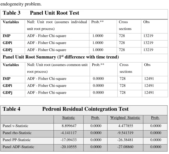
Before running our regressions we conduct a unit root and panel cointegration tests of the variables. The panel unit root results given in the table 3 show that the null hypothesis of unit root cannot be rejected. However, when we test for unit root with the 1st difference and time trend the null hypothesis of unit root can be rejected. This clearly indicates that the variables are integrated of order one which serves as a prerequisite for cointegration test.
Then we run Pedroni’s residual cointegration test to check for cointegration among variables. Pedroni cointegration test results show that the null hypothesis of no cointegration can be safely rejected for all 4 tests that have been discussed in the previous section. This enables us to use OLS and DOLS estimation methods since the estimated parameters are super-consistent. However, we prefer to use DOLS due to the potential endogeneity problem.
Table 3 Panel Unit Root Test
Variables Null: Unit root (assumes individual unit root process)
Prob.** Cross sections
Obs
IMP ADF - Fisher Chi-square 1.0000 728 13219
GDPi ADF - Fisher Chi-square 1.0000 728 13219
GDPj ADF - Fisher Chi-square 1.0000 728 13219
Panel Unit Root Summary (1st difference with time trend)
Variables Null: Unit root (assumes common unit root process)
Prob.** Cross sections
Obs
IMP ADF - Fisher Chi-square 0.0000 728 12491
GDPi ADF - Fisher Chi-square 0.0000 728 12491
GDPj ADF - Fisher Chi-square 0.0000 728 12491
Table 4 Pedroni Residual Cointegration Test
Statistic Prob. Weighted Statistic Prob. Panel v-Statistic 8.899647 0.0000 4.477855 0.0000 Panel rho-Statistic -4.141117 0.0000 -9.541319 0.0000 Panel PP-Statistic -17.09433 0.0000 -26.38481 0.0000 Panel ADF-Statistic -20.10555 0.0000 -27.08860 0.0000
18
5.2
Regression Results
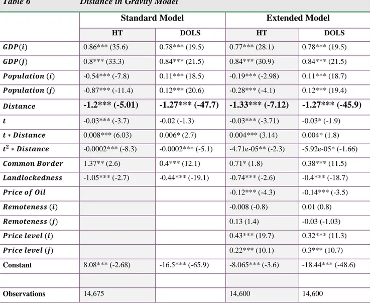
Table 6 presents the regression results for the standard and extended gravity models. In the standard gravity model the distance coefficient was equal to -1.2 in HT estimator and to -1.27 in DOLS method. These results are very close to the results obtained by Brun et al. (2005), Felbermayr and Kohler (2006), Coe et al. (2007). They also confirm the well-established negative effect of distance on international which is close to unity. Almost all of the estimated coefficients in the standard model are significant at 1% level. The GDP coefficients are positive and close to one as expected. This explains the fact that as income increases the consumption will increase and some part of this consumption will fall on imports ((McCallum (1995), Wei (1996)). The noticeable difference can be observed in the population coefficients with HT estimator indicating a negative impact on imports while the DOLS shows that they have a positive impact. There is no consensus on the role of population in the international trade. For example, Matyas (1997) and Bergstrand (1989) reported a positive impact of population on international trade while Dell`Ariccia (1999) found a negative impact. In contrast, Nuroglu (2014) states that the population should have a positive impact for the exporting country and negative impact for the importing country. However, in our case this coefficient is positive for both exporting and importing countries in DOLS estimation and negative (for both) in HT estimation. The elasticity of trade to common border in DOLS estimation is equal to 0.4, while in the HT estimation it is quite high (1.37). Our findings are in line with the findings of Helliwell (1997) and Nitsch (2000) who observed an increasing trade effect among the neighbouring countries.
The extended model produced similar results to the standard model. For example, the distance coefficient for DOLS in both cases is equal to -1.27 while in the HT estimator it is slightly higher -1.33. The fact that we have obtained very similar results indicates that the problem of omitted variable was not so severe. Although quite small (0.12 and -0.14), the price of oil has a negative significant impact on imports. Chinn (2008) and Bergin (2007) noted that oil prices have a direct impact on transportation costs. If the oil price increases, the cost of transportation will also increase and trade will decline. When the oil prices peaked in 2008, Krugman (2008) have stated that higher oil prices are putting brakes to globalization. In contrast, the remoteness index was found to have no significant impact on the trade. In addition to this, price level effect has been found to be
significantly positive. For example, 10% increase in the price level of the importing country would increase imports by 4.3% in HT estimation and 3.2% in DOLS estimation. The increase in the price level in the home country makes the domestic products relatively more expensive. Thus consumers and foreigners buy less of the domestic products and consume more of imported products which results in increase in imports (Arnold (2008)).
Table 6 Distance in Gravity Model
Standard Model Extended Model
HT DOLS HT DOLS 𝑮𝑫𝑷(𝒊) 0.86*** (35.6) 0.78*** (19.5) 0.77*** (28.1) 0.78*** (19.5) 𝑮𝑫𝑷(𝒋) 0.8*** (33.3) 0.84*** (21.5) 0.84*** (30.9) 0.84*** (21.5) 𝑷𝒐𝒑𝒖𝒍𝒂𝒕𝒊𝒐𝒏 (𝒊) -0.54*** (-7.8) 0.11*** (18.5) -0.19*** (-2.98) 0.11*** (18.7) 𝑷𝒐𝒑𝒖𝒍𝒂𝒕𝒊𝒐𝒏 (𝒋) -0.87*** (-11.4) 0.12*** (20.6) -0.28*** (-4.1) 0.12*** (19.4) 𝑫𝒊𝒔𝒕𝒂𝒏𝒄𝒆 -1.2*** (-5.01) -1.27*** (-47.7) -1.33*** (-7.12) -1.27*** (-45.9) 𝒕 -0.03*** (-3.7) -0.02 (-1.3) -0.03*** (-3.71) -0.03* (-1.9) 𝒕 ∗ 𝑫𝒊𝒔𝒕𝒂𝒏𝒄𝒆 0.008*** (6.03) 0.006* (2.7) 0.004*** (3.14) 0.004* (1.8) 𝒕𝟐∗ 𝑫𝒊𝒔𝒕𝒂𝒏𝒄𝒆 -0.0002*** (-8.3) -0.0002*** (-5.1) -4.71e-05** (-2.3) -5.92e-05* (-1.66) 𝑪𝒐𝒎𝒎𝒐𝒏 𝑩𝒐𝒓𝒅𝒆𝒓 1.37** (2.6) 0.4*** (12.1) 0.71* (1.8) 0.38*** (11.5) 𝑳𝒂𝒏𝒅𝒍𝒐𝒄𝒌𝒆𝒅𝒏𝒆𝒔𝒔 -1.05*** (-2.7) -0.44*** (-19.1) -0.74*** (-2.6) -0.4*** (-18.7) 𝑷𝒓𝒊𝒄𝒆 𝒐𝒇 𝑶𝒊𝒍 -0.12*** (-4.3) -0.14*** (-3.5) 𝑹𝒆𝒎𝒐𝒕𝒆𝒏𝒆𝒔𝒔 (𝒊) -0.008 (-0.8) 0.01 (0.8) 𝑹𝒆𝒎𝒐𝒕𝒆𝒏𝒆𝒔𝒔 (𝒋) 0.13 (1.4) -0.03 (-1.03) 𝑷𝒓𝒊𝒄𝒆 𝒍𝒆𝒗𝒆𝒍 (𝒊) 0.43*** (19.7) 0.32*** (11.3) 𝑷𝒓𝒊𝒄𝒆 𝒍𝒆𝒗𝒆𝒍 (𝒋) 0.22*** (10.1) 0.3*** (10.7) Constant 8.08*** (-2.68) -16.5*** (-65.9) -8.065*** (-3.6) -18.44*** (-48.6) Observations 14,675 14,600 14,600
*** significant at 1%, ** significant at 5%, * significant at 10% t-stats in parenthesis
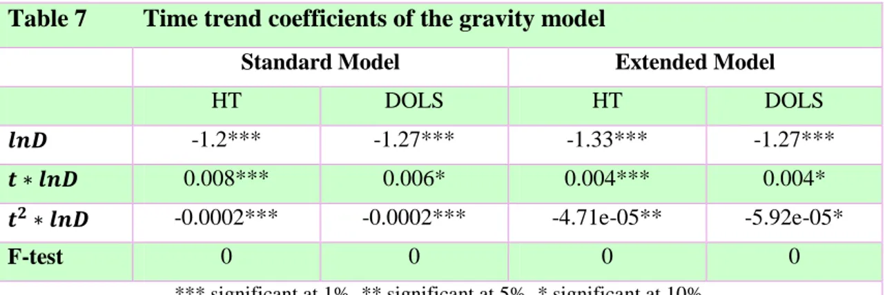
As it has been already mentioned we are mostly interested in the evolution of distance coefficient in this models. Thus we make use of the estimates of distance coefficient and time trend figures to show whether the importance of distance has increased or decreased
20
over the given time. To see how distance has evolved over time we construct an index by the use of the equation 22.
Table 7 Time trend coefficients of the gravity model
Standard Model Extended Model
HT DOLS HT DOLS
𝒍𝒏𝑫 -1.2*** -1.27*** -1.33*** -1.27*** 𝒕 ∗ 𝒍𝒏𝑫 0.008*** 0.006* 0.004*** 0.004* 𝒕𝟐∗ 𝒍𝒏𝑫 -0.0002*** -0.0002*** -4.71e-05** -5.92e-05*
F-test 0 0 0 0
*** significant at 1%, ** significant at 5%, * significant at 10%
Graph 1 shows how distance coefficient has changed over 20 year period in the standard gravity model. As you can see both of the estimation methods confirm the fact that the distance coefficient has declined over the chosen time. However, there are some noticeable differences between the two methods. First of all, DOLS line is above the HT line indicating that DOLS allocates higher significance to the distance in the gravity model. Moreover, in DOLS the distance coefficient falls from 1.27 to 1.15 representing almost 10% decline in the coefficient, while in HT the value of the coefficient falls from 1.19 in 1994 to 1.03 in 2014 representing a 13.5% decline proving that the distance coefficient falls faster in HT than in DOLS. Nevertheless, the values obtained in both estimations are within the range of the values obtained in the previous papers (0.8 and 1.5). In addition to this both estimations confirm the fact that the importance of distance has declined in international trade similar to the conclusions reached by Coe al. (2007), Larch et al. (2008), Brun et al. (2005).
Graph 2 describes the evolution of the distance coefficient in the gravity model when the extended model was applied. This time we can see the HT line above the DOLS line. The coefficient of distance in the HT method has declined from 1.33 in 1994 to just under 1.25 in 2014 representing a 6% decline, meanwhile the coefficient fell from 1.27 to 1.19 in DOLS also representing a 6% decline. If we compare the 2 estimation methods based
2 We substitute 𝛾
1with 𝑙𝑛𝐷, 𝛾2 with 𝑡 ∗ 𝑙𝑛𝐷 and 𝛾3 with 𝑡2∗ 𝑙𝑛𝐷 . We use time
values between 1994 and 2004 for the 𝑡 variable and calculate the index. Then we take the absolute values of the indices and draw a graph. Example for the Standard HT model: 𝛾𝑡= |−1.2 + 0.008 ∗ 𝑡 + (−0.0002)2∗ 𝑡|
on the standard and extended model results we can see that DOLS performs much better in comparison to HT estimator. The DOLS estimation of the distance coefficient has remained within the range of 1.15 and 1.27 in both specifications, while the HT estimator produced significantly different results for the specifications (between 1.19 and 1.03 for the standard model and between 1.33 and 1.24 for the extended model). One of the possible reasons for the difference in the two specifications might be the presence of omitted variable bias in the standard model. Adding more explanatory variables such as price of oil and price level to the standard specification has taken away some explanatory power from the distance coefficient which was a proxy for trade barriers and transport costs. In general, the decline in the distance coefficient is steeper in the standard model in comparison to the augmented one (which can also be deduced by comparing the slopes). Comparing the graphs and the distance coefficients of the 2 specifications we can come to conclusion that the standard model underestimates the distance coefficient. This is especially apparent in the case of HT estimator which has produced significantly different results for the 2 specifications.
HT DOLS 1 1.05 1.1 1.15 1.2 1.25 1.3 1992 1994 1996 1998 2000 2002 2004 2006 2008 2010 2012 2014 2016
22
There might be many reasons which have contributed to the declining importance of distance in international trade. Homayounnejad (2010) states that the decrease in the transportation and communication costs have contributed to the decline in the importance of distance in international trade. For example, the improvements in containerisation have reduced the sea transport cost by over 70% in the last 2 decades and air-freight cost have also been falling on average by 3% annually. According to WTO road transport costs have fallen by over 40% therefore increasing inland international trade. Another factor that has contributed to the increase in international trade within Europe is the introduction of the common currency Euro. Berger and Nitsch (2008) have estimated that international trade within EU members has increased between 5-20%. In addition to this, international trade has been further intensified by the formation of the regional trade agreements (RTA), which removes the tariff and quotas among the member countries. Since its foundation in 1995, WTO has received more than 200 notifications on either formation of new trading blocs or the accession of new states to the existing blocs.
HT DOLS 1.1 1.15 1.2 1.25 1.3 1.35 1.4 1992 1994 1996 1998 2000 2002 2004 2006 2008 2010 2012 2014 2016
6.
Conclusion
In this paper we have revisited the ‘’distance puzzle’’ in the gravity model applied to international trade practice of EU member states. The distance puzzle has been the outcome of the failure of the gravity model to reflect the falling trade related costs in the form of declining distance coefficient in the international trade. Most of the empirical research on distance puzzle concluded that the distance coefficient has remained either constant or increased (Head & Mayer, 2013).
Contrary to the mainstream results, we have been able to obtain declining distance coefficient in the gravity model applied to the bilateral trade data of 27 EU countries between 1994 and 2014. In our analysis we have used standard and extended specifications of the gravity model as suggested by Brun et al. (2005). Dynamic OLS and HT estimation approaches were employed to account for the endogeneity, spurious regression and selection bias problems associated with the panel dataset.
Our estimation results show that the importance of the distance coefficient in the gravity model of EU trade has fallen from -1.27 in 1994 to -1.15 in 2014 representing approximately 6% decline. The use of different model specification and different estimation methods changed slightly the values of the coefficients, however they didn’t alter the nature of the results. Hence, our results have proven to be robust to several ad hoc specifications and estimation methods. Thus, we can confidently conclude that the importance of distance in trade among EU states has declined over the last 2 decades. In addition to the distance estimate we have obtained significant results for the GDPs’ of the countries which were quite close to unity as it was expected. Moreover, Price of oil had a negative significant impact on the imports. Similarly, we had a negative sign for the dummy variable of being landlocked (which was also significant). In contrast, sharing a common border had a significant positive effect on the trade among the countries.
24
Reference
Anderson, E. (2011), The Gravity Model, Annual Review of Economics, vol. 3
Archanskaia, E. (2012), Heterogeneity and the Distance Puzzle, IMF working paper No
95
Baldwin, R., & Taglioni, D. (2006), Gravity for Dummies and Dummies for Gravity,
NBER Working Paper 12516, National Bureau of Economic Research
Baltagi, B. Bresson, G. Pirotte, A. (2002), Fixed effects, random effects or Hausman-Taylor? A pre-test estimator, Economic letters 79 (2003) 361–369
Behar, A. (2010), Transport costs and international Trade, University of Oxford
Department of Economics, No 488
Berthelon, M., & Freund, C. L. (2008). On the Conservation of Distance in International Trade, Journal of International Economics, vol. 75(2), pp. 310-320
Bleaney, M. (2012), Declining Distance Effects in International Trade: Some Country-Level Evidence, CREDIT Research Paper No. 11/02
Bolsso, D. (1998), Economic Distance, Cultural Distance, and Openness in International Trade: Empirical Puzzles, Journal of Economic Integration, Pages 156-184.
Brun, J., Carre`re, C., Guillaumont, C. (2005), Has Distance Died? Evidence from a Panel Gravity Model, The World Bank Economic Review, Vol. 19, No. 1, pp. 99–120
Buch, C. (2003), The Distance Puzzle: On the Interpretation of the Distance Coefficient in Gravity Equations, Kiel Working Paper No. 1159
Bussière, M. (2008), EU Enlargement and Trade Integration: Lessons from a Gravity Model, Review of Development Economics, 12(3), 562–576
Bussière, M., Fidrmuc, J., Schnatz, B. (2005), Trade integration of central and eastern European countries. Lessons from a gravity model, European Central Bank Working
paper series. No. 545
Chaney, T. (2011), The Gravity Equation in International Trade: An Explanation,
University of Chicago, NBER and CEPR.
Cheong, J. (2011), The Distance Effects on the Intensive and Extensive Margins of Trade over Time, School of Economics, University of Queensland
Christie, E. (2002), Potential trade in southeast Europe: a gravity model approach, WIIW
Coe, D. (2007), The Missing Globalization Puzzle: Evidence of the Declining Importance of Distance, IMF Staff Papers Vol. 54, No. 1
Davidová, L. (2014), Various Estimation Techniques of the Gravity Model of Trade,
Charles University in Prague Faculty of Social Sciences Institute of Economic Studies
Deardorff, A. (1998), Determinants of Bilateral Trade: Does Gravity Work in a Neoclassical World? National Bureau of Economic Research
Egger, P., & Pfaffermayr, M. (2003), The Proper Panel Econometric Specification of the Gravity Equation: A Three-Way Model with Bilateral Interaction Effects, Empirical
Economics, vol. 28
Head, K., & Mayer, T. (2013), Gravity Equations: Workhorse, Toolkit, and Cookbook.
CEPII Working Paper 2013-27
Máthyás, L. (1997), Proper Econometric Specification of Gravity Model, The World
Economy, vol 20., pp. 363-368
Megi, M. (2014), The Gravity Model on EU Countries – An Econometric Approach,
European Journal of Sustainable Development (2014), 3, 3, 149-158
Neumann, I. (2014), Impacts of the integration on trade of EU members – a gravity model approach, The central European journal of regional development and tourism, Vol. 6
Issue 1
Pedroni, P. (2001), Purchasing Power Parity Tests in Cointegrated Panels, The Review of
Economics and Statistics, MIT Press, vol. 83(4), pp. 727-73
Redding, S. (2003), Distance, Skill Deepening and Development: Will Peripheral Countries Ever Get Rich? Centre for Economic Performance
Riaz, M. (2005), Theoretical Groundwork for Gravity Model, Proceedings of 3rd
International Conference on Business Management
Rose, A. (2000), One Money, One Market: Estimating The Effect of Common Currencies on Trade, Economic Policy, pp. 7-45
Salvatici, L. (2013), The Gravity Model in International Trade. African Growth and
Development Policy modelling consortium
Serlenga, L., & Shin, Y. (2004), Gravity Models of the Intra-EU Trade: Application of the Hausman-Taylor Estimation in Heterogeneous Panels with Common Time-specific Factors, Edinburgh School of Economics Discussion Paper Series. 105
Serlenga, L., & Shin, Y. (2007). Gravity Models of Intra-EU Trade: Application of the CCEP-HT Estimation in Heterogeneous Panels with Unobserved Common Time-Specific Factors, Journal of Applied Econometrics , Vol. 22, No. 2
26
Stack, M. (2010). Regional integration and trade: A panel cointegration approach to estimating the gravity model, The Journal of International Trade & Economic
Development Vol. 20, No. 1, February 2011, 53–65
Tayyab, M., Tarar, A., Riaz, M. (2012), Review of gravity model derivations,
Mathematical Theory and Modeling, Vol.2, No.9
Vancauteren, M., & Weiserbs, D. (2012), Intra-European Trade of Manufacturing Goods: An Extension of the Gravity Model, International Econometric Review
Woytek, K. (2003), Of Openness and Distance: Trade Developments in the Commonwealth of Independent States, 1993–2002, IMF Working Paper 03/207
Yotov, Y. V. (2012), A Simple Solution to the Distance Puzzle in International Trade,
Economics Letters, vol. 117(3), pp. 794-798
Zwinkels, R. C., & Beugelsdijk, S. (2010), Gravity Equations; Workhorse or Trojan Horse in Explaining Trade and FDI Patterns Across Time and Space? International
Appendix 1
List of EU countries
Austria Germany Netherlands
Belgium Greece Poland
Bulgaria Hungary Portugal
Croatia Ireland Romania
Republic of Cyprus Italy Slovakia
Czech Republic Latvia Slovenia
Denmark Lithuania Spain
Estonia Luxembourg Sweden
Finland Malta UK
28
Appendix 3
Descriptive Statistics of the Data
IMP GDPI GDPJ POPI POPJ DIS
Mean 3.08E+09 4.91E+11 4.65E+11 1.80E+07 1.69E+07 1.84E+03
Median 2.98E+08 1.58E+11 1.39E+11 8.84E+06 8.30E+06 1.72E+03
Maximum 1.19E+11 3.87E+12 3.87E+12 8.25E+07 8.25E+07 5.13E+03
Minimum 28000000 3000000000 3000000000 367941 367941 80
Std. Dev. 9.45E+09 7.94E+11 7.95E+11 2.25E+07 2.22E+07 993.92
Skewness 5.84 2.19 2.31 1.52 1.71 0.54
Kurtosis 45.45 7.09 7.52 4.01 4.58 2.83
Jarque-Bera 1.19E+06 2.20E+04 2.56E+04 6.30E+03 8.68E+03 7.41E+02
Probability 0 0 0 0 0 0