Economic Impact of Microcredit in an Urban Setting
The Case of Tajikistan
Bachelor’s Thesis within Economics Authors: Manizha Kodirova
Shabnam Mirzoeva Tutors: James Dzansi Erik Wallentin
Bachelor’s Thesis in Economics
Title: Economic Impact of Microcredit in an Urban Setting: The Case of Tajikistan Author: Manizha Kodirova, Shabnam Mirzoeva
Tutors: James Dzansi, Erik Wallentin
Date: May, 2012
Key terms: Tajikistan, microcredit, income change, urban poverty, difference-in-differences
Abstract
This paper investigates the impact of receiving microcredit on the economic conditions of urban poor. The change in household income level between the years 2009 and 2011 was measured for a group of survey participants half of whom were microcredit benefi-ciaries, while the other half were not. The survey was conducted in Dushanbe, the capi-tal city of Tajikistan. A difference-in-differences approach was used for the analysis and various other attributes that influence income such as the level of education, age and gender were taken into account in model formation. The findings indicate that micro-loans do not significantly affect the income level of the urbn poor in the short run.
Table of Contents
1
Introduction ... 3
2
Background ... 4
2.1 The Keynesian Consumption Function ... 4
2.2 The Permanent Income Hypothesis ... 6
2.3 The Life-Cycle Hypothesis ... 7
2.4 The Evolution of Microfinance ... 7
2.5 Microfinance sector in Tajikistan ... 9
2.6 Previous Impact Studies ... 10
3
Methodology ... 11
3.1 Survey design and data collection ... 11
3.2 Descriptive Statistics ... 12
3.3 Model Formation ... 14
4
Results and Analysis ... 16
4.1 Regression Results ... 16
4.2 Analysis of the Findings ... 17
5
Conclusion ... 19
5.1 Suggestions for further studies ... 19
References ... 21
Figures
Figure 2.1 Consumption Income Relations………….………..………..6
Figure 3.1 Consumption of survey participants……….13
Figure 3.2 Average income level of survey participants……….…..14
Tables
Table 3.1 The role of coefficients in the regression model 1…………..………...…16Table 4.1 Regression output. Dependent variable: Income level for years 2009 and 2011………..…….17
Table A1 Microcredit and Microdeposit services in Tajikistan as of January 2009…...24
Appendices……….………...24
Appendix 1………....24
Appendix 2………25
1
Introduction
While there are continuous attempts to combat poverty in the developing world, no single technique has yet succeeded in reducing world poverty at a large scale. Microfinance, when it came about, was widely perceived as a way to accomplish this by including the income con-strained poor in the financial markets. It refers to a range of financial services such as savings, loans and insurance, aimed at serving low-income clients, particularly women, with little or no access to traditional financial services (The MIX, 2012). The size of loans tends to be very small and since they are targeted at poor individuals, non-conventional collateral and contrac-tual means are used. These small loans are known as microcredits and what made them unique is the innovative use of joint liability groups (JLG). This refers to group lending methods, where the group acts as a form of social collateral. The idea is that if one group member de-faults, the rest of the group will be denied access to further loans. This ensured that lending in-stitutions would achieve returns while the availability of credit would be a sustainable source of financing to the recipients. Therefore, in the past three decades, microfinance programs have been growing in size and number in developing and transition economies and have been prac-ticed differently, albeit their success rates have varied.
Empirical impact studies show mixed results concerning microfinance as a means to poverty alleviation. Independent studies conducted by the World Bank have documented positive ef-fects of microcredits on the poor customers of the Grameen Bank (Yunus, 2002). At the same time many other studies show cases where users of microfinance services have become far worse off than before (Bateman, 2010).
This paper aims to investigate whether or not the use of microcredit improves the economic situation as measured by the income level of the micro-borrowers in urban areas of Tajikistan. There are several reasons for this. First, most impact studies on microfinance as a means to fight poverty centre around rural areas despite the fact that in almost all developing and transi-tion economies, large portransi-tions of urban dwellers also live in poverty (World Development In-dicators, 2012). In Tajikistan, which is one of the poorest countries in the world located in Cen-tral Asia, 21.5 percent of urban dwellers live on less than 1.25 dollars a day – the World Bank defined poverty line (ADB report, 2011). Thus, an urban area assessment will contribute to bet-ter understanding the full extent of microfinance impacts.
Additionally, MFIs have only recently began to establish in Tajikistan thus few impact studies have been conducted. According to the World Bank, in 2010, 47 percent of the country’s popu-lation lived below the poverty line and the per capita GDP in 2010 was 2190 current dollars (Global Finance, 2012). This poverty came about suddenly after the collapse of the Soviet Un-ion in the late 1980s. Gaining independence in 1991, the country was almost immediately en-gulfed in a civil war (1992-1997) that damaged the economy. As a result, over 80 percent of the population suddenly fell into poverty after a century of stable growth and development un-der the Soviet rule (ADB, 2011; Falkingham, 2000). As one of the ways to combat this pov-erty, microfinance institutions (MFIs) were introduced as of 2004 (AMFOT, 2012)1. To test whether these MFIs have improved the economic situation of the urban poor, we look into the household income changes of a group of microcredit beneficiaries between the years 2009 and 2011. In order to put this change into context, the income level changes of a comparable con-trol group were also measured. These measurements were attained through a survey of 49
1 AMFOT – The association of Microfinance Organizations in Tajikistan – is the national microfinance
association in Tajikistan that works with microfinance institutions and governments in helping them with strategic decision-making processes through cooperation within the various sectors.
rower and 50 non-borrower households. The survey also obtained information on various other attributes that affect income levels, for instance, gender, age, and education. Then a difference-in-differences model was applied to single out the effect of microcredit. The results indicate that taking microloans do not significantly improve household income levels. Gender and age on the other hand, do have significant influence on the income level, while a higher level of education has no substantial benefit.
The remainder of the paper is structured as follows. Section 2 gives a theoretical framework about credit constraint and the need for microfinance services among the poor. It also provides a background to the evolution of microfinance, its development in Tajikistan as well as previ-ous impact studies on microfinance. Section 3 displays the data collection and processing methodology. Section 4 provides the results and the analysis, while section 5 gives the con-cluding remarks.
2
Background
Before discussing the role of microfinance in delivering credit especially to the poor to im-prove their economic situations, we must first show that the poor do in fact demand financial services and that providing such services as savings and credit will help them out of poverty. Credit is obtained to finance consumption of some sort or investment (in human or physical capital). When investment is the purpose of borrowing, it is usually expected to generate mon-ey returns. Greater monmon-ey returns imply higher future income, which in turn raises consump-tion and utility. There is a close connecconsump-tion between investment, income level and consumpconsump-tion and thus living standards.
This section describes various economic theories that elucidate how increased income level can raise consumption and the role of credit in stimulating this increase when households are fi-nancially constrained. The three theories to be discussed are the Keynesian consumption func-tion, Friedman’s permanent income hypothesis (PIH), and Modigliani’s life-cycle hypothesis (LCH). All these models share some common assumptions. First, it is assumed that individuals (or households) are rational beings with predictable responses to changes in incentives and that they attempt to maximise their utility. Second, the models assume that income levels fluctuate over time, so to ‘smooth’ their consumption levels, individuals/households may save or borrow in different points in time. Finally, it is assumed that households base their consumption choices on income, therefore, household behaviour is dependent on expected income. We now describe these models and their relevance to the role of microfinance. We then go on to discuss some theories of microfinance that came about to meet the demand for financial services by the poor.
2.1
2.1 The Keynesian Consumption Function
Keynes argues that households make the factors of production they possess available to firms, which use them to produce goods and services. In return for the use of these factors of produc-tion, firms pay households. This payment is income. For most households, income consists of
the wages and salaries they receive, or profits they generate from their own business activity, in return for their labour. This income is used to buy goods and services (Godley, 1999).
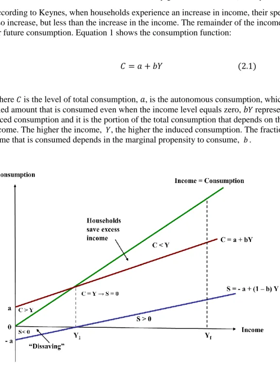
According to Keynes, when households experience an increase in income, their spending will also increase, but less than the increase in the income. The remainder of the income is saved for future consumption. Equation 1 shows the consumption function:
Where is the level of total consumption, , is the autonomous consumption, which is the fixed amount that is consumed even when the income level equals zero, represents the in-duced consumption and it is the portion of the total consumption that depends on the level of income. The higher the income, , the higher the induced consumption. The fraction of in-come that is consumed depends in the marginal propensity to consume, .
Figure 2.1: Consumption Income Relations
(Adapted from Ando & Modigliani, 1963)
The portion that is not consumed is saved to raise future consumption. Saving is equivalent to investment and it can be derived from the consumption function of equation ( ):
In Figure 2.1, marginal propensity to save is represented by The portion of income that is saved or invested is equal to . At point , households consume all their income. Above that point, they have enough to save/invest. But if their income is below , households consume more than they earn as their autonomous consumption is above their income level. They pay off the excess consumption either from their savings, or, if they have no savings, by borrowing. Most poor households tend to have income levels below . This means that their need for borrowing is higher than those of better-off households, who have excess income to save. As Coleman (1999) puts it, one of the causes for poverty in the developing world is the lack of access to productive capital. As a result, low income households are faced by a vicious cycle. They only produce/earn at a subsistence level, meaning they consume all that they pro-duce, making it impossible to accumulate capital by saving or through other assets. Therefore, they are unable to invest in productive resources that would allow them to generate more in-come or gain access to credit in formal capital markets to raise their long term inin-come and con-sumption levels.
2.2
2.2 The Permanent Income Hypothesis
The PIH was developed by Friedman (1957) to explain household consumption behaviour shown by empirical studies, but unexplained by the Keynesian consumption model. What the Keynesian theory fails to explain is that households with lower income levels tend to have higher average propensity to consume in the short run than those with higher incomes, but over the long run, the average propensity to consume is constant irrespective of differences in in-come levels.
The PIH explains this behaviour by assuming that the aggregate income level is composed of two separate components: permanent (projected) income level, . and transitory income level, , which simply represents the unexpected changes in income. That is, = + . It is as-sumed that short run income fluctuations are normally distributed meaning that .This implies that in the long run, = .
The final assumption is that consumption level is positively related to permanent income:
, such that represents long run aggregate consumption behaviour and k is the mar-ginal/average propensity to consume. This means, change in permanent income level changes the consumption level.
The implication of the model is that in the short run there is a difference between transitory and projected income levels, but that consumption levels remain more or less constant. So when + is positive, households tend to save. When this difference is negative, households smooth their consumption by living off their previous savings. If they do not have sufficient savings, then households will borrow (and they expect to repay their borrowing debt with higher in-come in the future) (Friedman, 1957). Poor households are generally in the situation where their income is below their autonomous consumption. Where unemployment is prevalent and no opportunities for improving income situations exist, there is a crucial need by the poor to borrow. Microcredit is not only demanded to meet current consumption, but also acts as a source of investment into an income generating activity with returns in the future (both short-run and long-short-run). The focus of this paper is to study this impact in the short short-run.
2.3
2.3 The Life-Cycle Hypothesis
Modigliani and Brumberg’s (1954) well known LCH predicts that an individual’s consumption patterns over his or her lifetime are interlinked with income levels and thus create demand for saving and borrowing.
The model predicts that individuals maximise their utility gained from present consumption,
as well as a stream of future consumptions, , subject to present income level, , ex-pected future income levels, and initial wealth, , which can be put into productive use. The model, in its general form can be written as:
where is the utility derived from the consumption level at time t; is the income re-ceived in time period t; r is the current interest (the price of spending money today as opposed to saving it) and ρ is the rate of time preference that measures the to what extent the current consumption levels are favoured over future ones. If ρ is high, current consumption is preferred to future consumption, therefore, households spend all their current income. On the other hand, if ρ is low, higher consumption levels in the future are preferred and households save some of their current incomes. We assume that ρ is constant in the short run.
Equation ( ) can be re-written as:
where is the utility derived from current consumption. A high ρ would imply that for a given level of > , so that current consumption is to the detri-ment of the future ones (Ando & Modigliani, 1963).
It is assumed that poorer individuals or households tend to have higher ρ than those who are wealthier. This assumption stems from the fact that most of the income of poor households are expended on basic needs, whereas better-off households are more likely to have excess income to save. As a result, there exists high demand for credit services among the poor. Microfinance is one possible source of credit that helps overcome these credit constraints. The next section presents some theories and facts in this regard.
2.4
2.4 The Evolution of Microfinance
The previous section indicated that there exists demand for credit among the poor. However, supplying formal credit and depositing services to the poor have historically proven to be a challenge. Commercial banks have always tended to shy away from delivering credit and
de-pository services to the very poor in developing countries due to the high risks and high trans-actions costs associated with small loans and deposits (Coleman, 2006). The poor, having very low level of capital per person, find themselves trapped in poverty. The capital is accumulated when households save a part of their income. This saving can either be lent to banks or invest-ed directly into own or other businesses (equities tradinvest-ed in the market) (Sachs, 2005) However, as a result of low level of capital, all of the poor’s income is spent on consumption, therefore leaving them with no personal savings to invest.
Many governments have attempted to deliver formal financial services to the poor through set-ting up various programs such as agricultural banks. However, these have proven unsuccessful due to low repayment rates and the unwillingness of governments to impose strict rules on the already financially constrained (Adams, Graham, & von Pischke, 1984). Microfinance, was widely perceived as a solution to this problem of marginalisation of the poor from the financial market. It originated as microcredit rather than microfinance in Bangladesh in the late 1970s by Muhammad Yunus, who gave out small loans mostly to the very poor women with the aim to help them out of poverty trap. He used the concept of group lending whereby borrowers were asked to form a group of around five people and were only able to continuously borrow as long as each group member repaid loans on time. That is, group members had joint liability, which acted as collateral. Over time banks giving out microcredits also began to provide other finan-cial services such as insurance and depository services, hence the development of the term mi-crofinance.
This concept of group lending makes microfinance unique since it is said to overcome the problem of information asymmetries, that is, lack of accurate client information required by lending institutions to ensure repayments are made when they give loans without collateral. Specifically, information asymmetries cause adverse selection and moral hazard problems. Adverse selection occurs when the lender is not well-informed about the riskiness of its bor-rowers. The riskier a borrower, the higher the possibility of default. In the presence of moral hazard, the lender is unable to assess whether or not the borrower utilises the loan in the ex-pected use as agreed upon in the lending contract. Thus in the absence of collateral, lenders have difficulty incentivising borrowers to make timely repayments or make repayments alto-gether. Moreover, the lender cannot know if the borrower puts in the necessary inputs, espe-cially efforts needed to increase their chances of repaying the loan (Duvendack, et al. 2011). Proponents of microfinance including Yunus (2002) reason that joint-liability groups resolves the problem of information asymmetry by means of peer monitoring and pressure to encourage repayments. For this reason, the workings of group lending and its benefits for lenders have been the focus of theoretical model building in the field of microfinance.
The best known theory on microfinance is Stiglitz and Hoff’s (1990) group lending model where they argue that the local borrowers (assumed to know one another) are the ones who monitor their peers since if their peers (group members) default, the rest of the group will not be able to get further loans either. Assuming self-selection, Stiglitz and Hoff argue that group formation will lead to positive assortative matching (that is, risky borrowers will group with other risky borrowers, while the safe will team up with safe). As a result, the risk of default is shifted from the bank to the borrowers, who then either help their peers in repayment in times of need or threaten to place social sanctions if they find that their peers are shirking. The threat itself, it is claimed, will be enough pressure to prevent shirking and unnecessarily defaulting (Armendariz de Aghion, Morduch, 2005). This way the group lending model is a way out of the adverse selection issue.
With the expansion of microfinance and its demonstrated profitability in the early stages, many profit-maximising investors began to capitalise MFIs that initially relied highly on grant and government subsidies for survival. Thus the quest for financial self-sustainability led to mass commercialisation of the MFIs in the late 1990s (Bateman, 2010). Moreover, these institutions expanded their target market to serve more than just those living below poverty line. Group lending as the main means of collateral is now no longer the norm as it has not always proved successful in preventing default rates. Instead, those taking larger loans on an individual basis place assets as collateral. Nevertheless, both social collateral (group lending) and other forms are in use today.
The commercialisation of microfinance is a topic of controversy, especially given the case of Compartamos Banco – Mexico’s largest microfinance bank, which was the first to sell its shares to the public as an attempt to become financially sustainable. The results were charging extremely high interest rates on loans, which hindered the ability of loan repayment and even-tually led to a crisis. (Bateman, 2010).
2.5
2.5 Microfinance sector in Tajikistan
The motivating factor to start microfinance programs in Tajikistan was to encourage economic activity and impede spiraling poverty and further marginalisation of the poor (Venkatachalam, 2005). Another reason was to reduce dependence on remittances, which, since the collapse of the Soviet Union, accounts for about half of the country’s GDP (World Bank report 2012). The reason for the dependence on remittances is the high unemployment level in the country. This is due to the sluggishness in economic and entrepreneurial activities caused by various factors including high corruption which makes doing business difficult (Doing Business ranked Tajiki-stan as 147 out of 182 countries in 2012), soviet era infrastructure and factories that have not been upgraded and are thus either out of function or extremely inefficient (and would account for thousands of jobs) and weak education system. There are also geographical factors that play an important role in high unemployment and poverty rates, for example, the country is land-locked with extremely high mountains making up 93 percent of the area. These make agricul-tural and other industrial activities difficult. Finally, the meager amount of naagricul-tural resources further contributes to persistent poverty.
The first MFI to operate in Tajikistan was Aga Khan Foundation’s First Microfinance Bank (FMFB) in 2004 (FMFB, 2012). In 2009, involved in microfinance services were 12 (conven-tional) commercial banks, 88 MFIs and seven credit societies operating in Tajikistan. In 2010, the total amount of loan outstanding amounted to 417.7 million USD. This amount was bor-rowed by 133,619 customers, meaning the average loan size was about 3,127 USD (MIX mar-ket publication).2
The microfinance market in Tajikistan is smaller compared to that of other Central Asian coun-tries3. Majority of the microfinance banks are small (i.e. serve less than 10,000 borrowers), ex-cept for only six institutions that have more than 10, 000 consumers4, and these account for over 7.5 percent of the total micro loans borrowers (AMFOT, 2009). It must also be noted that
2
MIX or Microfinance Information Exchange is a nonprofit organization that provides financial and so-cial performance data from MFIs. Along with the Microcredit Summit, it is the largest provider of data on microfiance. Information is obtained from service providers and networks and investors.
3
Tajikistan microfinance market in the context of Central Asia ( Appendix)
4
urban lending is slightly less prevalent in Tajikistan than rural lending and accounts for 44 per-cent of all microloans.
Table A1 in the Appendix 2 indicates that majority of microfinance services in Tajikistan are carried out by non-bank providers, primarily by MFIs. Statistics from MIX and AMFOT indi-cate that there are generally more micro-borrowers than depositors. This is attributed to the country’s weak financial system, due to which many have little trust in financial institutions. As a result, the clients of MFIs (as well as the general public) prefer to invest their income back into their businesses or save money in hard currencies (MIX and AMFOT, 2009).
Prior to assessing the impact of microcredit on income level of households in Tajikistan, it is imperative to look at some previous studies that discuss the effects of microcredits.
2.6
2.6 Previous Impact Studies
Studies on the impacts of microfinance intervention on income and other welfare measures are mixed and most argue that assessing such impacts is extremely difficult.
Chen and Mahmud (1995) purport that the assumption that the effect of credit is brought about merely through the changes experienced in business income is specious. The direct and indirect changes it can bring to household relationships and roles, attitudes, and cognitive effects are all equally profound (Chen and Mahmud, 1995; Scheffer, 2009). Nevertheless, most investiga-tions assessing the influence of credit on poverty reduction use cause-and-effect models where credit is used as an exogenous treatment variable and the changes it causes on a few indicators of well-being, such as income, are measured (Duvendack, et al. 2011). Researchers of micro-finance struggle to disentangle the role of microloans on income and other situational changes the borrowers may experience. It has been repeatedly proven that microfinance participants have higher income levels (or are wealthier in general) prior to using microfinance services (see for example Coleman, 2002; Alexander, 2001; and Hashemi (1997). The results of this study also support this point.
In an extensive study of group lending in North Eastern Thailand, Coleman (1999) finds that the impact of microcredit intervention on various welfare measures not necessarily positive. He finds for instance that obtaining a microloan had insignificant impact on production, sales, sav-ings, labour time, physical assets, health care and education. Moreover, his study results indi-cate that microcredit had a significant effect on further indebting female borrowers. This was the result of many women falling into a vicious cycle of debt from local money lenders as a means to be able to repay their village bank loans. Interestingly, he also finds significantly pos-itive relationship between microcredit intervention and women lending out money with interest since some members took microloans from village banks at low interest rates and lent them out at mark-up to benefit from arbitrage. Therefore, Coleman concludes that first, there is no evi-dence that microloans are being put into productive use to generate returns. Second, he argues that debt is not an effective method for improving the economic conditions of the low-income households, rather the poor are poor due to other reasons than credit access.
A study by US Agency for International Development (USAID) to examine whether or not borrowing has benefitted the poor, shows mixed results. USAID (2002) undertook three paral-lel studies in SEWA’s Bank in India, Mibanci’s in Peru and Zambuko’s Trust in Zimbabwe. The study concluded that although microfinance makes a difference, no single impact was found uniformly in all three targeted countries. It resulted in not all borrowers experiencing
rowers in Zimbabwe for instance, had lower average incomes to those who did not borrow af-ter inaf-tervention. However, there was limited evidence that participation in microfinance pro-grams had very negative impact on these households, except perhaps extreme poor households who were highly indebted. Furthermore, taking out a microloan encouraged diversification of income sources in Peru and Zimbabwe, but not in India. At enterprise level, in Peru and India microenterprises had significantly benefited from microfinance, whereas in Zimbabwe where many participants were not micro-entrepreneurs, the finding extended to all forms of informal sector earning. Moreover, in Peru, the use of microcredit led to positive impacts on enterprise revenues in spite of recession during the study period, while no impact of revenue was found on household enterprises in Zimbabwe or on clients primary enterprise in India. Households, particularly in India and Zimbabwe suffered from frequent and varied financial shocks, howev-er the assessment found showed limited capability of the households to cope with the shock expect for a slight increase in India.
Finally, Mosley (1996) studies the impacts of microfinance on the borrowers of Bolivia’s BancoSol. This study shows that in any given cohort, about a quarter of the loan beneficiaries experienced significant gains as a result of borrowing, while about 10 to 15 percent suffer loss-es and the vast majority (60 to 65 percent) saw no changloss-es in their income situations.
Given the mixed results shown by previous studies about the impact of microcredit on the wel-fare of the poor in various developing countries, we expect ambiguous results for the case of Tajikistan. The following sections depict our findings.
3
Methodology
This section is divided into three parts. The first part gives an overview of the survey design and collection of the data. The second part discusses the descriptive statistics based on the pro-file of the participated households. The last part describes the model formation methods ap-plied in this study.
3.1
3.1 Survey design and data collection
A survey was conducted in March 2012 in Dushanbe, the capital and prime city (the main ur-ban area) of Tajikistan. Of the 99 selected survey participants, 49 were microloan recipients, while the other 50 were non-recipients. To ensure that data collection was as random as possi-ble, surveys were conducted outside six different MFIs in Dushanbe (with their permission). The reason for choosing to survey in these locations was to maximise the chances of coming into contact with microcredit users while at the same time meeting enough non-borrowers. Data were collected on annual household income level, profession, education, and gender of the household income earners, whether or not a microloan was taken by any household mem-bers and how much. This was done to ensure that the treatment group (micro-borrowers) and the control group (non-borrowers) were as comparable as possible.
Out of 72 microloan borrowers interviewed, 49 of them were used in the analysis because the rest did not meet the eligibility criteria such as having initial monthly income levels between 150-500 USD or residing in Dushanbe for the past three years. Non-borrowers were also
ap-proached in the same location, and their selection was dependent on the same criteria as the microloan borrowers to make them comparable as required by our research.
The reason we chose the income range of 150 to 500 USD per month (which accumulates to 1800 USD to 6000 USD per year) was because the lower bound is about the same as the aver-age GDP per capita for the years 2009-2011, while the upper bound takes into account those who were earning just above GDP per capita. This group of people stand just above the poverty line and are able to afford the collateral required to take microloans, but still do not have easy access to conventional financial services.
Regarding location, all survey participants lived in the prime city, Dushanbe during the years 2009-2011. This location was chosen because, as mentioned previously, it is Tajikistan’s larg-est urban area. This is in line with the purpose of the paper, which is to assess microcredit im-pacts in an urban setting.
The surveys were conducted in Tajik and Russian , which are spoken in Tajikistan. Both quali-tative and quantiquali-tative data were collected. The names of the beneficiaries as well as non-borrowers were not registered for reasons of anonymity. Low sample size (only 99 responded in total) is one of the main limitations of this study, which was due to time constraint. Never-theless, the sample size is sufficient in shedding light into the possible income differences caused by microcredit intervention.
3.2
3.2 Descriptive Statistics
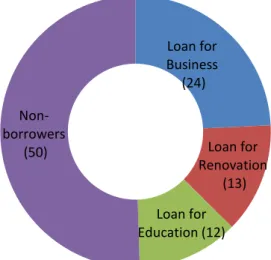
Figure 3.1 displays the composition of survey participants. Out of the 99 respondents, 50 had taken no loans and from the 49 who had, over half had taken business loans while the remain-ing either borrowed to finance children’s education or to renovate a house/apartment in order to later hire it out. Thus all groups of borrowers expect future returns with the difference being that those taking business loans expect their returns in the short run (within a year or so), while those renovating their property on credit expect to generate returns in the medium term and the borrowers for their children’s education expect to reap the benefits of credit in the long run.
Figure 3.1: Composition of survey participants 2011. Loan for Business (24) Loan for Renovation (13) Loan for Education (12) Non- borrowers (50)
The profile of the participating household was based on the head of the household’s age, gen-der, occupation and income level. There were more female participants in the survey than male ones. Out of the 49 respondents in the treatment group, 29 of them were females, making up 60% of the borrower respondents. Similarly, the control group consisted of 52% females. All of the participants surveyed had at least completed secondary education (and 80% held a uni-versity degree), were between the ages of 21 and 65 and made significant contribution to their household income. The number of dependent family members of the interviewees were be-tween one and four persons. The number of income earners in the households was two or three. Moreover, the household members’ occupation ranged from tailors, teaching, dentistry and bank employees to business occupations such as taxi drivers, tailors, retailers and bakers. As Figure 3.2 shows, there is some – though not significant – difference in the average income levels of different groups of borrowers as well as non-borrowers both before and after the mi-crocredit intervention. Users of business loans had the highest initial income (4450 USD per annum) and income level after the intervention (5435 USD). They also experienced the biggest change in income over this time span. Borrowers for renovation had lower average income lev-el in 2009 than those who borrowed for business or for education, but in 2011, they had the se-cond highest average income level (3814 USD initially and 4324 USD in 2011). Overall, those who borrowed to finance children’s education experienced no income change – as indicated by Figure 3.2, there is almost no average difference. About half of these borrowers saw marginal increase in their income levels between the two years, while for the remaining, their income levels fell. In the survey, all these borrowers associated the fall in their income to loan repay-ment. Those who had taken no loans had the lowest level of income both before and after the intervention (average of 3598 USD and 3791USD respectively). Their average increase in in-come was only a little over 5 percent, a sharp contrast to borrowers for business who, on aver-age, saw their income levels increase by more than 22 percent or borrowers for renovation whose income level increased on average by over 13 percent.
When asked about their overall quality of life had changed after taking out a loan, 77 percent of the borrowers felt they were better off. The remaining 23 percent claimed to have become worse off, as they did not have sufficient means to cover their loans and had to borrow from other MFIs, friends and family to repay them. Of these, most had borrowed to finance their children’s education.
In addition, the results from interviewing non-borrowers indicated that 44 percent were una-ware of the existence of MFIs. Another 26 percent had no interest in taking loans due to high interest rates and the remaining 30 percent had no collateral means. The type of collateral (or wealth) placed by those who did borrow were immovable property, car or jewellery, depending on the size of the loan.
It is also interesting to note that the size of the different types of loans varied. Although micro-finance banks offer a wide range of loan size of all types, those borrowing for education had the smallest loans ranging from 400 USD to 1300 USD, whereas those borrowing to renovate took larger loans ranging from 700 USD to 2100 USD. Business loans have the largest range from only 200 USD to 2500 USD though on average they were smaller than those who took renovation loans (1006 USD and 1400 USD respectively).
Figure 3.2: Average income levels of survey participants in 2009 and in 2011. (Constructed by the authors from survey data).
With regards to age, most borrowers of education and reconstruction loans were in their late forties, while business loan takers and non-borrowers were in their early forties or late thirties. On a final note, there were equal number of females and males, who took business loans. This is interesting to point out since microfinance has, since its beginnings, advocated for targeting poor female entrepreneurs.
3.3
3.3 Model Formation
As an attempt to disentangle the role of microcredits in changes in income level from other in-fluencing factors, we use the difference-in-differences method. This method has the ability to measure the delivered changes due to a treatment, when faced with data limitations and the im-possibility of having a counterfactual. As argued by Armendariz de Aghion & Morduch (2005), accurately estimating the impact of microloan on borrowers must entail not only con-trolling for the roles of measurable attributes such as age, profession, education and experi-ence, but also holding constant some unmeasurable attributes that affect income changes, for instance, entrepreneurial ability, political upheavals, economic booms or inflation rates at the time when the loans were taken. Furthermore, it is argued that any fixed individual-level and macroeconomic effect will eventually even out during the differencing procedure.
In our data collection, we have obtained the measurable attributes mentioned above, but lack the unmeasured, which we assume to be the same across all survey participants. This approach works well in terms of accurately measuring the causal effect of microfinance only if observa-ble and unobservaobserva-ble attributes in treatment and control groups are time-invariant. However, this assumption does not always hold in practice since attributes are bound to change over time (Armendariz Aghion and Morduch, 2005).
The average treatment on the treated can be calculated by letting be a households in-come of the treatment group before taking out a loan and their income after taking out the microloan. Similar is the case for the control group with and representing their
0 1000 2000 3000 4000 5000 6000 Year 2009 Year 2011
The impact we are measuring is the mean change in income caused by borrowing a loan, writ-ten as:
which depicts the change in household income of borrowers minus the change in income of non-borrowers for 2009 and 2011.
The above DD approach can be depicted in a regression form as shown in model 1:
where Yi is an income level for observation i for years 2009 and 2011; represents being a
borrower, i.e. it equals one when the observation is a borrower and zero otherwise; is a dummy variable that takes a value of 1 for observations in year 2011. Its purpose is to control for exogenous changes in the economic and social environment that are hard to observe, such as inflation, economic booms/recessions or political upheavals that have an impact on income changes. It is difficult to predict whether this variable will have a positive or a negative impact on income since much of its attributes are unmeasurable. It is included in the model to find out if these exogenous factors improved or worsened household economic situations. Since the control group plays the role of the counterfactual for the borrowers, the coefficient of this dummy is roughly equal to the average difference in the income level of non-borrowers be-tween 2011 and 2009.
The simple DD regression of model 1 can be augmented by including additional explanatory variables with an impact on income level.
where agei dummy variable signifies those participants who are at or above 40 years of age. It
equals zero otherwise. Since individuals generally acquire more knowledge, experience and as-sets that generate financial returns over time, income is expected to rise with age, thus this var-iable should have a positive impact on income level; genderi dummy variable represents
fe-male heads of households. In developing countries such as Tajikistan, being a fefe-male head of household is associated with lower income level, thus this variable is expected to be negatively related to income level; educationi dummy variable depicts those interviewed who held a
uni-versity degree as opposed to those who completed secondary education (none of the partici-pants had less than a secondary school degree). The education level is expected to be positively related to income level. A higher level of education is associated with more knowledge and qualifications for better paid jobs.
Table 3.1 The interpretation of the coefficients in the regression model 1
Treatment Group Control Group Difference
Before +
After + + + + +
Difference +
The DD approach is popular in academia, but not without flaws. Heckman (1997) and Khandker (2010) advocate combining DD approach with matching methods as it would help to account for selection on observable and unobservable indicators by comparing outcomes of participants and matched non-participants before and after treatment effect. However, this also assumes that observable and unobservable attributes in both groups are time-invariant, which is not always the case.
4
Results and Analysis
This section presents the results obtained from the regressions. We investigate the impact of a microloan as well as other measurable attributes on the income level of borrowers and non-borrowers for years 2009 and 2011. The analysis is carried out based on the theories presented in section 2.
4.1
4.1 Regression Results
Two regressions were performed on the regressand, household income level (Yi), for the years
2009 and 2011. The predictor variables are all dummy variables and include: being a borrower, time dummy (2011), DD, age, gender and education level. Both regressions treat the same 99 observations of the survey. The results are displayed in Table 4.1.
The first model is the simple DD approach in a regression form. Here the intercept, , repre-sents the average income level of the non-borrowers before the microcredit intervention or treatment effect. Accordingly, this figure equaled 3597,60 USD per annum.
The treatment coefficient, , which represents the initial income differences between the two groups is statistically insignificant at 5 percent level. Similarly, the coefficient , which cap-tures income differences of non-borrowers over the study period and which is equivalent to the DD estimate of the treatment effect are statistically insignificant at 5 percent level.
Three additional variables, age, gender and education level are included in the extended DD model. As expected, age (being 40 years old or above) has a positive, statistically significant impact on income level and gender (being a female income earner) has a negative, significant
effect. However, the impact of education level (having a university degree as opposed to only completing secondary school) is positive, but statistically insignificant.
The F-statistic for both regressions is significant indicating that at least of one of the variables in every regression is significantly different from zero. The R-squared is low in both cases. In model 1 for instance, it is only 0, 057 indicating that the explanatory variables explain only 5.7 percent of the variation in the income level. The adjusted R-squared value for model 2 is 0,113. Including measurable attributes, such as age, gender and education increased the adjusted R-squared implying that the model 2 is a better predictor.
Table 4.1 Regression output.
Dependent variable: Income level for years 2009 and 2011
Variables (1) (2) Constant 3597,60 (16,260) 3428,16 (10,628) Borrower Dummy 455,46 (1,448) 273,44 (0,831) Time Dummy 193,00 (0,617) 193,00 (0,059) DD 381,29 (0,588) 371,10 (0,099) Age 764,42 (0,234)* Gender -455,11 (-0,139)* Education 168,68 (0,051) R2 0,057 0,140 R2adj 0,042 0,113 F-statistic 3,890 5,18 Number of observations: 99 * = p-value <0,05
The figures in parentheses indicate the t-statistics
4.2
4.2 Analysis of the Findings
The results of this study demonstrate that overall, microcredit has no significant impact on in-come level of the urban poor in the short run. The result from the difference-in-differences model indicates that users of microcredit do not experience significantly higher increases in their income levels than those who take no loans.
Moreover, we must not dismiss the fact that borrowers may have been better off in terms of their level of wealth, which is not accounted for in the models above. Wealth acts as collateral to obtain a loan: in this study, all borrowers claimed that they were obliged to place a collateral that was at least twice the money value of their loan size. The great majority of non-borrowers surveyed stated that the reason they did not take a microloan was because they did not have the collateral means. There are two implications to this result: one the demand for credit is very high among the urban poor (as indicated by the theories of PIH and LCH), and two the finan-cially excluded poor remain excluded in the urban areas. Group lending may be a solution here, however, microfinance has evolved so much to resemble conventional financial sector today that group lending is hardly practiced in general, particularly in urban areas.
The insignificant coefficient for the ‘Time Dummy’ showing the change in income of non-borrowers from 2009 to 2011 implies that there was no marked change in the income level of those who did not take out a loan. This makes intuitive sense since income does not usually change considerably in such a short time period. Another purpose of this variable is to capture the changes in income levels resulting from exogenous influencing factors unmeasured by the study such as an economic fluctuation or a political upheaval. The insignificant result is an in-dication that those unmeasured aspects remained more or less constant.
As the coefficient of the DD variable, 3, is statistically insignificant, we conclude that the im-pact of microcredit on income level is not sufficiently large, at least during the period of study. This is because depending on the type of loan taken (for example, a consumer loan or a busi-ness loan), the time it takes to see the impacts on the income situation of the borrower varies. In the case of a business loan for instance, which is invested into the borrower’s small or medi-um sized enterprise, the effects tend to become apparent within a year or so. On the other hand, loans taken to invest in the children’s education may take many years before there is a measur-able impact and even then it can be hard to pinpoint.
Many of the survey respondents who took education loans claimed that although they experi-enced little or no improvements in their income situations over the survey period, they ex-pected future returns once their children complete their education, begin earning income and finance the household. The reasoning behind the three different types of borrowers (business, renovation and education purposes) and their ability to generate returns can be explained using Modigliani’s life-cycle hypothesis. Why is it that although borrowing to fund children’s educa-tion may take many years before any returns are apparent, heads of households take credit to finance this? And why is it that other households, especially the ones that own businesses pre-fer to see immediate improvements in their income levels? The life-cycle hypothesis purports that variations in individuals’ or households’ time preference for consumption explains their saving, investment and borrowing behaviours. That is, those who prefer to consume higher levels now than in the future (those with high time preference rates) tend to be those who pre-fer high current returns. Borrowers of business loans can be placed in this category. By the same token, one would expect those taking education loans to have lower time preferences, meaning that they invest in the future at the expense to income and consumption levels today. The fact that the majority of borrowers took business and renovation loans is coherent with the theory that most urban poor, like rural poor, have high time preference rates, that is, they prefer high current consumption to high future consumption.
The positive impact of age on income can be ascribed to the fact that individuals acquire knowledge, experience as well as assets over time that give money returns. The higher asset
to provide collateral twice the money value of their loans). Therefore, being able to borrow larger loans, especially to invest in a business, is likely to lead to higher profits (and thus to higher income levels) than smaller loans.
The fact that the gender dummy is negative is as expected and there are several reasons that can explain this. First, it may be due to discrimination: that women are paid less than men. Discrimination is the case in most developing countries and one of the initial purposes of mi-crofinance was to eradicate it. Another reason why women earn less than men may be that due to their traditional roles in Tajikistan, they dedicate far more time on non-income generating household activities than men. Less time spent on income generating activities naturally means less income.
5
Conclusion
This paper assesses the possible impact of microloans on the income levels of the urban poor residing in Tajikistan. The findings imply that microcredit does not significantly improve household income in the short run. The survey results confirm the stylised facts that only households with income levels well above the poverty line had access to microcredit. These households also had income levels higher than the national per capita GDP. This implies that an average resident with income level equal to the national average is likely to have no access to microcredit, at least in the urban areas. Moreover, the purpose of the loan makes a difference in the extent of short run impacts. Entrepreneurial borrowers benefit more from microcredit than those who take credit to invest in education or renovation.
The findings question the role of microcredit as a means to reduce poverty and enhance gender equality. Clearly, gender inequality remains an issue when comparing income differences in spite of the microcredit intervention. Ironically, the very poor are discriminated from accessing credit due to their lack of collateral. It seems, microcredit is beneficial to what can be referred to as the ‘better-off’ poor: those who have sufficient means to sustain themselves, but to be able to further improve their economic conditions, they need access to credit. Since the size of loans they require are relatively small, they do not have access to traditional financial institu-tions. Therefore, microcredit is one of the few sources of credit for this group of people. In this sense, microfinance can be seen as a positive intervention as it provides access to credit to those in need. However, as long as the sole goal of MFIs is profit maximisation, meaning that the cost to the clients of borrowing will be very high, microcredit is less likely to help the des-perately poor, who are financially excluded. MFIs with a combination of social and commer-cial goals that set affordable prices and are more client-oriented may have better impacts on the income levels of all borrowers. Moreover, these benefits will be optimal when combined with other measures such as governmental investment in education, infrastructure and health care among others.
5.1
5.1 Suggestions for further studies
Although this study gives a fair indication of the change in income situation due to microcredit intervention, there are limitations. Lacking from this study was the availability of data - only a small number of loan beneficiaries and non-beneficiaries were surveyed (i.e. 99 people). In
ad-dition, data were only collected for two years (cross sectional data), whilst the impact of a loan can take years to show. Thus, further studies that measure the various impacts of microcredit over a longer period with larger number of survey participants from various urban regions not only in Tajikistan, but throughout Central Asia will lead to better understanding the true im-pacts of microfinance on the urban poor. In addition, it would be of interest to conduct research that compares the effect of the treatment over rural and urban regions. Finally, limitations to this study exist in the explanatory variables measured. As opposed to grouping borrowers into two different education level criteria and two different age groups, perhaps the results would have been more accurate if age was treated a continuous variable, and if a different measure-ment was used for education. Adding more explanatory variables must be obtained from more thoroughly surveys.
References
Adams, D., W., Douglas H., Graham and J.D. Von Pischke, eds. (1984) Undermining
Rural Development with Cheap Credit. Boulder, Colorado: Westview Press.
Ando, A. and Modigliani, F. (1963) The “Life Cycle’’ Hypothesis of Saving: Aggregate Impli-cations and Tests. The American Economic Review, Vol. 53, No. 1, Part 1. pp. 55-84.
Angrist, D. & Pischke, J. (2009) Mostly harmless econometrics, an empiricist’s companion. Princeton: Princeton University Press
Armendariz de Aghion, B & Morduch, J. (2005) The economics of Microfinance. The MIT Press, Cambridge, MA.
Asian Development Bank (2011) Asian Development Bank and Tajikistan Fact Sheet. Re-trieved April 20, 2012. http://www.adb.org/publications/tajikistan-fact-sheet.
Asian Development Bank (2010) Asian Development Bank Report 2010. Retrieved April 19, 2012. http://www.adb.org/documents/adb-annual-report-2010.
Association of Microfinance Organizations of Tajikistan (2010). Analysis of AMFOT
mem-bers activity in 2010. Retrieved April 20, 2012.
http://amfot.tj/en/microfinance/analysis_of_amfot_member/
Banerjee,A. & Duflo,D.(2010) Giving Credit Where it is Due. Retrieved from: econom-ics.mit.edu/files/5415.
Bashar, T. and Rashid,S., (2010) Urban microfinance and urban poverty in Bangladesh.
Jour-nal of the Asia Pacific Economy, pp. 151-170.
Bernasek, A. (2003) Banking on social change: Grameen bank lending to women.
Internation-al JournInternation-al of Politics, Culture and Society, Vol. 16, No. 3 Spring 2003.
Chen, M., and Mahmud, S., (1995) Assessing change in women’s lives: a conceptual
frame-work. Working paper No 2, BRAC-ICDDR, Joint Research Project and Matlab, Dhaka.
Coleman.B. (2006) Mocrofinance in Northeast Thailand: Who benefits and how much? World
Development. Vol. 34, No. 9, pp. 1612–1638. doi 10.1016/j.worlddev 2006.01.006
Duvendack M., Palmer-Jones R., Copestake JG., Hooper L., Loke Y. and Rao N. (2011) What
is the evidence of the impact of microfinance on the well-being of poor people? London:
EPPI-Centre, Social Science Research Unit, Institute of Education, University of London.
Friedman, M., (1957) A Theory of the Consumption Function. Princeton University Press, Princeton.
Ghatak, M. and Guinnane, T. (1999) The economics of lending with joint liability: theory and practice. Journal of Development Economics 60, pp. 195– 228.
Ghatak, M. (2000) Screening by the company you keep: joint liability lending and the peer se-lection effect. Economic Journal 110. pp. 601–631.
Global Finance (2012) The Poorest Countries in the World. Retrieved April 17, 2012. http://www.gfmag.com/tools/global-database/economic-data/10502-the-poorest-countries-in-the-world.html#axzz1qWX2y8VI
Godley, W. (1999) Money and credit in a Keynesian model of income determination.
Cam-bridge Journal of Economics, 23, pp.393-411.
Goetz, A. and Sen Gupta, R. (1996) Who takes credit? Gender, power, and control over loan use in rural credit programs in Bangladesh. World Development, 24(I), pp. 43-63.
Hermes N. and Lensink R. (2007) The empirics of microfinance: what do we know? The
Eco-nomic Journal, 117 (517): F1-F10.
Hoff, K. and Stiglitz J.(1990) Moneylender and bankers: Price increasing subsidies in a mo-nopolistically competitive market. Journal of Development Economics. Vol. 55. No 2. pp. 485-518.
Hulme, D. and Mosley, P. (1996) Finance Against Poverty. London: Routledge.
Kempson, E. and Whyley, C. (2000) Kept Put or Opted Out? Understanding and Combating
Financial Exclusion. Policy Press, Bristol.
Mayo E, Fisher T., Conaty P., Doling J,Mullineux A. (1998) Small is Bankable. Community
Reinvestment in the UK New Economics Foundation. Cinnamon House, 68 Cole Street,
Lon-don SE1 4HY.
Mayoux L. (1997) “The Magic Ingredient? Microfinance and Women’s Empowerment”. A Briefing Paper prepared for the Micro Credit Summit, Washington.
Microfinance Information Exchange (MIX) & Association of Microfinance Organizations of Tajikistan (2009) Tajikistan 2009: Microfinance analysis and benchmarking report. Retrieved from: http://www.themix.org/publications/mix-microfinance-world/2009/12/2009-tajikistan-microfinance-analysis-and-benchmarking-r
Modigliani, F. and Brumberg, R. (1954) Utility Analysis and the Consumption Function: An Interpretation of Cross-Section Data. In Post-Keynesian Economics ed. K. Kurihara. New Brunswick: Rutgers University Press.
Morduch, J. (1998) Does Microfinance really help the poor? Evidence from Flagship Pro-grams in Bangladesh. Hoover Institution, Stanford University Press.
Morduch, J. (2000), The Microfinance Schism, World Development, Vol.28, No.4, pp. 617-629.
Morduch, J., Kunt A. and Cull R. (2009) Microfinance meets the market. Journal of Economic
Perspectives. Volume 23, Number 1.Pages 167–192.
Mosley, P. (1996) Metamorphosis From NGO to Commercial Bank: The Case of
BancoSol in Bolivia. pp. 1-31
Pitt, M. and Khandker S.R. (1998) The impact of Group-Based Credit Programs on Poor Households in Bangladesh: Does the Gender of Participants Matter? Journal of Political
Econ-omy, 106.
Rogaly, B., Fisher, T., and Mayo, E. (1999). Poverty social exclusion and microfinance in
Britain.Oxfam: Oxfam GB and New Economics Foundation
Sachs, J. (2005). The End of Poverty: Economic Possibilities for Our Time. New York: Pen-guin Books.
Scheffer M. (2009) Critical transitions in nature and society. Princeton University Press. Sen, A. (1999) Development as Freedom. Oxford University Press.
Shahinpoor, N. (2009) The link between Islamic Banking and Microfinancing. International Journal of Social Economics, Vol.36, No.10, pp. 996- 1007.
Sinclair, S.P. (2001) Financial Exclusion: An Introductory Survey, Center for Research into
Socially Inclusive Services (CRSIS). Edinburgh.
Sobhan, R.. (2010) Challenging the injustice of poverty: agenda for inclusive development in
South Asia. London: Sage.
Stiglitz,J. (1990) Peer monitoring and credit markets. World Bank Economic Review. Vol 4. No.3. pp 351-366.
The Microcredit Summit Organization (2009) State of the Microcredit Summit
Cam-paign2012..Retrieved.from:
http://www.microcreditsummit.org/pubs/reports/socr/2012/WEB_SOCR-2012_English.pdf UNCDF Brandsma J., Burjorjee D. (2004) Microfinance in the Arab States. Building inclusive
financial sectors.
UNDP: Human development indices - Table 3: Human and income poverty (Population living below national poverty line (2000-2007). Retrieved April 10, 2012.
World Bank Organization (2012). Retrieved April 4, 2012.
http://data.worldbank.org/country/tajikistan
Wright, G. (2000) Microfinance Systems: Designing Quality Financial Services for the Poor. Zed Books, London.
Wright, K. (2006) The darker side to microfinance: evidence from Cajamarca, Peru. New York, Routledge.
Yunus, M. (2002) Grameen Bank II: Designed to open new possibilities. Dhaka:Grameen Bank. Retrieved from: www.grameen-info.orf/bank/bank2.html
Appendices
Appendix 1
Table A1 Microcredit and Microdeposit services in Tajikistan as of January 2009
Legal Status Profit
Status Status Legal Institutions Number of Number of borrowers Portfolio in thous. USD Balance, USD Avg.Loan Microloan Fund Non-Profit NBFI 41 67, 316 19, 048 283 Microloan Organization Profit NBFI 37 62, 773 47, 930 764 Microdeposit Organization Profit NBFI 14 23, 705 12, 178 514
Credit Union Profit Credit Union 7 401 1, 935 2, 475 Specialized Microfinance Bank Profit Bank 1 13, 153 32, 550 2, 475 Downscaling Banks Profit Bank 4 33, 290 114, 799 3, 377 Total 104 201,338 228, 441 1, 135
Appendix 2
Tests on model 2
In order to test whether Model 2 is a good estimation, we ran tests for normality, multicollinearity and heteroscedasticity.
1) Cook’s Distance Test for normality
One of the prerequisites to run a regression is that each disturbance term has normal distribu-tion i.e. normality assumpdistribu-tion. It can be summarized as:
where N represents normal distribution and the terms in the parentheses indicate the mean val-ue of 0 and the variance.
In order to test for normality , Cook’s Distance is conducted with the results presented in Table X. The assumption of normality is violated when the values of Cook’s Distance are high. Ac-cording to Tabachnick and Fidell (2007) the values of Cook’s Distance that are close to 1 would indicate serious problem. As seen in Table 4.3 the Cook’s Distance values are rather low in this analysis, therefore suggesting the assumption of normality to hold.
Table A2 Cook’s Distance Test for Model 2
Cook's Distance Max. 0,064
2) White’s General Heteroscedasticity Test
Homoscedasticity is present in the regression model when all random variables have the same finite variance. In other words, variances of the residuals are constant for all observations. To test for homoscedasticity, White’s General Heteroscedasticity test is performed:
The test hypothesis is:
H0 : Homoscedasticity
H1 :Heteroscedasticity
According to the table A3, the obtained chi-square is value for the regression is 27,9. The criti-cal chi-square value with a probability of 0.01 and 14 degrees of freedom is equal to 29,14. As the result , [Xobs = 27,9] < [Xcrit = 29,14]. The null hypothesis can not be rejected meaning there is no severe problem of heteroscedasticity present in Model 2.
Table A3 : White’s Test
Obs*r-squared 27,9 Prob. Chi-square 0,0028
3) Variance Inflating Factor (VIF) – test for multicollinearity
The problem of multicollinearity appears in the model if there is a correlation between the in-dependent variables, as the result of which the coefficient estimates become inefficient but un-biased. According to Gujarati’s rule of thumb, if VIF > 10, there is a serious problem of multicollinearity present in the model. By looking at VIF estimates of model 2, it can be con-cluded that the explanatory variables are less than 10, meaning that multicollinearity is not a big problem.
Table A4: Variance Inflating Factor for regression model 2
TimeDummy 1,980 Interaction Term 2,980 Gender 1,044 Age group 1,178 Education 1,342
Appendix 3
Below is the survey questionnaire that was given out to the survey participants in March 2012. When conducting the survey, the questionnaire was translated into Russian and Tajik, which are the main languages spoken in Tajikistan.
QUESTIONNAIRE
1. Age:
Under 25 25-40 Above 40 2. Gender: Male Female
3. Marital Status: Single Married Divorced Widowed
4. Number of dependent family members (children, parents, etc -if any) 5. Level of education completed:
a) Primary b) Middle school c) Secondary
d) College/University
6. Did you have a stable source of income before you took out a microloan? (i.e. do you re-ceive money regularly?)
Yes No
7. What was (were) your main source(s) of income before you first took out a microloan? You can choose more than one box.
a) remittance payment from abroad b) salary from work
e) other, please specify………
8. What was your average monthly income before taking out loans? a) Under TJS200 b) TJS 200-500 c) TJS501-800 d) TJS801-1200 e) TJS1201-1600 f) TJS1601+
9. Are you a first time borrower? Yes No
10. How much did you borrow the first time? (Please specify the amount in Tajik Somonis/USD)
11. How much did you borrow the subsequent times (if appropriate)? 12. What was your reason for borrowing the FIRST TIME?
a) to start up own business b) to repay debt
c) to repair house
d) other personal or family reasons (e.g. medical, wedding, etc) 13. How long has it been since your first loan?
14. How long has it been since your last loan (if applicable)? 15. How often do you pay interest?
16. How much interest do you pay?
17. Have you been able to make all your interest payments on time?
18. If you took out a business loan, what line of business do you own? (E.g., bakery, sewing, retailer, etc,)
19. If non-business owner, what is your profession?
20. What did you deposit as collateral when taking out your FIRST loan? (e.g., money, house, animals, crop)
21. What was/were your collateral worth (in money terms)?
22. What is your average monthly income AFTER taking out loans? a) Under TJS 100
b) TJS 100-400 c) TJS 401-800 d) TJS 801-1200 e) TJS 1201-1600
f) TJS 1601+
23. Do you receive a regular income after taking out the loan(s)? Yes No
24. Have you borrowed from more than one bank? Yes No
25. Would you say your financial situation has improved after taking out loans? Yes No
26. How much time did it take you to prepare all the paperwork? 27. How much money did it cost you to prepare all the paperwork?