Transfer Learning for Machine Diagnostics

(1)

Master Thesis

HALMSTAD

UNIVERSITY

Master's in Information Technology, 120 credits

Transfer Learning for Machine Diagnostics

Information Technology, 30 credits

Halmstad 2020-09-05

(2)

C O N T E N T S 1 i n t r o d u c t i o n 2 1.1 Motivation 5 1.2 Problem statement 6 1.3 Challenges 7 1.4 Contribution 8 2 r e l at e d w o r k 10 3 m e t h o d 15

3.1 Proposed Network (DANN): 15 3.2 Ensembling Approach 16

3.3 Complete Network Architecture 24 3.4 Transfer Learning Scenario/Approach: 26

4 s y s t e m i m p l e m e n tat i o n 27

4.1 Pneumatic System Description 27 4.2 Data Collection Settings / Procedure 30 4.3 Exploratory Data Analysis 30

4.4 Feature Engineering and Transformation: 34

5 r e s u lt s 37

5.1 Results Evaluation Criteria 37 5.2 Experiments Summary 38 5.3 Experimental Results: 40 6 c o n c l u s i o n a n d f u t u r e w o r k 57 7 d i s c u s s i o n 59 b i b l i o g r a p h y 60 ii

(3)

L I S T O F F I G U R E S

Figure 1 Machine learning vs Transfer learning [1] 4 Figure 2 Basic Neural Network 13

Figure 3 Basic DANN Workflow 14 Figure 4 First Feature Extractor 18 Figure 5 Second Feature Extractor 19 Figure 6 Feature Extractors Ensemble 22

Figure 7 Proposed Network (DANN) Architecture 25 Figure 8 Pneumatic Reference System 27

Figure 9 Controlling System 27 Figure 10 Air Pressure Sensor 28 Figure 11 Air Flow Sensor 28 Figure 12 Regulator Valve 29 Figure 13 Dataset 31

Figure 14 Features Relationship (Healthy Data) 32 Figure 15 Features Relationship (Un-healthy Data) 33 Figure 16 AirFlow Comparison between healthy and

un-healthy data 33

Figure 17 AirFlow feature Skewness and Transformation 35 Figure 18 Features Correlation 36

Figure 19 SVM [Left: Case I ; Right: Case II] 40 Figure 20 Logistic Regression [Left: Case I ; Right: Case

II] 41

Figure 21 Naive Bayes [Left: Case I ; Right: Case II] 41 Figure 22 Random Forest [Left: Case I ; Right: Case II] 42 Figure 23 MLP (Sklearn) [Left: Case I ; Right: Case II] 42 Figure 24 CORAL [Left: Case I ; Right: Case II] 43 Figure 25 Results Summary 44

Figure 26 TL Setting 1: DANN disabled 48

Figure 27 TL Setting 1: Domains Data Representation (DANN Disabled) 48

Figure 28 TL Setting 1 DANN enabled 49

Figure 29 TL Setting 1: Domains Data Representation (DANN Enabled) 49

Figure 30 TL Setting 2: DANN disabled 50

Figure 31 TL Setting 2: Domains Data Representation (DANN Disabled) 50

Figure 32 TL Setting 2: DANN enabled 51

Figure 33 TL Setting 2: Domains Data Representation (DANN Enabled) 51

(4)

List of Figures iv

(5)

L I S T O F TA B L E S

Table 1 Different Settings of Transfer Learning [1] 3 Table 2 Individual Feature Extractors Predictions 20 Table 3 AirFlow Statistics 34

Table 4 Different Architectures with different Activa-tion FuncActiva-tions 45

Table 5 Heterogeneity Measuring Parameters 46 Table 6 Individual features extractors and ensembling

results 53

Table 7 Ensemble vs Feature Extractor 1 54 Table 8 Ensemble vs Feature Extractor 2 54 Table 9 6x6 Matrix [DANN Disabled] 55 Table 10 6x6 Matrix [DANN Enabled] 56

(6)

A C R O N Y M S

ART: Adaptive Resonance Theory

ANFIS: Adaptive Network-based Fuzzy Inference Systems

AUC: Area Under ROC Curve ANN: Artificial Neural Network

AE: Auto-encoder

BP: Back Propagation

BLSTM: Bi-directional Long Short-Term Memory

CNN: Convolutional Neural Networks CORAL: Correlation Alignment

DBN: Deep Belief Network

DBM: Deep Boltzmann Machines

DANN: Domain Adversarial Neural Networks

FE: Feature Extractor

IID: Independent and Identically Distributed

LVQ: Learning Vector Quantization

LSTM: Long Short-Term Memory

MLP: Multi-layer Perceptron

mSDA: Marginalized Stacked Denoising Autoencoders

ROC: Receiver Operating Characteristic

RNN: Recurrent Neural Networks

RUL: Remaining Useful Life

SoH: State of Health

SVM: Support Vector Machine

TAT: Transferable Adversarial Training

(7)

A B S T R A C T

Fault detection and diagnostics are crucial tasks in condition-based maintenance. Industries nowadays are in need of fault identification in their machines as early as possible to save money and take pre-cautionary measures in case of fault occurrence. Also, it is beneficial for the smooth interference in the manufacturing process in which it avoids sudden malfunctioning. Having sufficient training data for in-dustrial machines is also a major challenge which is a prerequisite for deep neural networks to train an accurate prediction model. Transfer learning in such cases is beneficial as it can be helpful in adapting different operating conditions and characteristics which is the case in real-life applications. Our work is focused on a pneumatic system which utilizes compressed air to perform operations and is used in different types of machines in the industrial field.

Our novel contribution is to build upon a Domain Adversarial Neural Network (DANN) with a unique approach by incorporating ensembling techniques for diagnostics of air leakage problem in the pneumatic system under transfer learning settings. Our approach of using ensemble methods for feature extraction shows up to 5 % improvement in the performance.

We have also performed a comparative analysis of our work with conventional machine and deep learning methods which depicts the importance of transfer learning and we have also demonstrated the generalization ability of our model. Lastly, we also mentioned a prob-lem specific contribution by suggesting a feature engineering approach, such that it could be implemented on almost every pneumatic sys-tem and could potentially impact the prediction result positively. We demonstrate that our designed model with domain adaptation ability will be quite useful and beneficial for the industry by saving their time and money and providing promising results for this air leakage problem in the pneumatic system.

(8)

1

I N T R O D U C T I O N

With the advancements in machine learning, there are ways that show up to transfer knowledge between multiple tasks. By transferring the knowledge gained in one task which is referred to as the source do-main(Xs)and using it to develop and improve learning in a somehow

similar task in which it is referred to as the target domain(Xt),

trans-fer learning attempts to show improvements compared to traditional machine learning methods. The more the target task is similar and related to the source task, the more it is mastered easily. In other words, the difference varies between the source domain and the target domain depending on the case or situation studied. In our case, the dif-ference between the source and the target domains is the air pressure operating settings. For example, having the source domain operating on 0.1 air pressure in the pneumatic system and the target on 0.5 air pressure in the same pneumatic system is less different than having the source as air pressure operating settings of a pneumatic system and the target as a nitrogen operating settings of a totally different pneumatic system or even a totally different task such as having the target as an image classification task which is entirely different from the source. It is always a great incentive to find ways of using data from one problem that generalizes to another because in applying machine learning, the cost of labeled data generated for a new task is often an obstacle. By the use of an extra set of unlabeled training data for the new task we wish to generalize, domain adaptation tries to achieve such a transfer.

Transfer learning can be in different settings such as transductive and inductive transfer learning, based on different situations between the target and source domains and tasks. As shown in table 1, in transductive transfer learning setting, the target and source tasks are the same, and a lot of labeled data in the source domain are available while no labeled data are available in the target domain. Whereas in inductive transfer learning setting, the source task is different from the target task, and some labeled data are required in the target domain that leads to an objective predictive model.

(9)

i n t r o d u c t i o n 3

Table 1: Different Settings of Transfer Learning [1]

Transfer Learning Settings Related Areas Source Domain Labels Target Domain Labels

Inductive Transfer Learning Multi-task learning Available Available Self-taught learning Unavailable Available Transnductive Transfer Learning Domain Adaptation, Available Unavailable

Sample Selection Bias, Co-variate Shift

This idea of domain adaptation is implemented in neural network architectures that are trained from the source domain(Xs)with labeled

data and unlabeled data from the target domain(Xt)[15]. In our case

for the pneumatic system, our source domain (the lab equipment) is labeled data whereas the target domain (equipment in the industries) has unlabelled data which is the case of transductive learning.

Transfer learning is useful when you have insufficient data for a new domain that you want to handle by machine learning methods and there is a big pre-existing data pool that can be transferred to your problem. Lacking of data that reflects the real usage of the equipment in application domain. e.g for electric buses do not have sufficient information. The behavioural characteristics of batteries in electric buses can depict variation due to different environment and operating conditions. Moreover, there are three main research issues in transfer learning that can arise:

• what to transfer: which part of the knowledge can be transferred from the source to the target in order to improve the performance of the target task. We try to identify which portion of knowledge is source-specific and what is common between the source and the target.

• how to transfer: After knowing the knowledge that can or should be transferred, developing the learning algorithms is needed for knowledge transfer which corresponds to the ”how to transfer” case. There can be scenarios where transferring knowledge for the sake of it may make matters worse than improving anything (also known as negative transfer)

• when to transfer: which situations, transferring skills, ways of ac-tually transferring the knowledge across domains/tasks should be done in order to avoid unexpected target task performance degradation since in some situations transferring knowledge can make things worse than improving anything.

Recently, Domain Adversarial Neural Networks (DANN) have been applied for fault diagnosis and machine prognosis. The idea is to train a deep neural network for extracting domain-invariant features

(10)

i n t r o d u c t i o n 4

that have predictive power for the classification/regression task e.g real-world applications, which might be very different from the source domain, e.g. controlled experiments. DANN includes a deep feature extractor and a label predictor, which is a standard architecture for performing supervised learning. The unsupervised domain adapta-tion task is carried out by a domain classifier, which backpropagates gradients for making features domain-invariant. As long as the pre-dictions applied on the data can not differentiate between the target (test) domain and the source (train) domain the more effective domain transfer is achieved.

The main objective of our work is to improve or build upon a Domain Adversarial Neural Networks (DANN) based method for fault detection under transfer learning settings, e.g. designing network structure and activation functions, for diagnosis of the pneumatic system, using multivariate time series data. Given a time series:

T={T1, T2, ...., Tn} Where ; T∈R

The proposed method will be evaluated using both simulated data and real data of the pneumatic systems coming from the industries. By adversarial, it is meant that the adversarial way of training is referring to source classifier competing against domain classifier in adversarial fashion, in other words, the model should work equally well on both datasets[18].

As a general and simple definition, transfer learning is a machine learning technique where knowledge gained during training in one type of problem is used to train in other similar type of problem and related tasks as shown in figure1. More technically, given a source domain Dsand learning task Ts, a target domain Dt and learning task

Tt, transfer learning aims to help improve the learning of the target

predictive function ft(.) in Dtusing the knowledge in Dsand Ts, where

Ds 6= Dt or Ts 6= Tt. That means that we do not have to start from

scratch with a model because we can use the model that we have and try it on similar task knowing what? why? and how? to transfer.

(11)

1.1 motivation 5

1.1 m o t i vat i o n

Most manufacturers that aim to stay competitive and powerful in the market need to follow the technological shifts and changes in addition to the need to automate their facilities. For pneumatic systems, when these kinds of systems face a problem, it leads to a significant increase in cost and in some cases the manufactured parts could be most probably wasted. This emphasizes the idea of how important it is to detect the problems and faults with their source as fast and precisely as possible to be aware of the consequences and to go on with the operating process with minimum interruption.

The problem which we aim to solve is regarding the compressed air leakage for the pneumatic system. When there exists some air leakage in the pneumatic system, it requires air compressors to work more which results in a significant increase in the operational cost. Moreover, it disturbs the functionality of the system as it does not behave on the desired air pressure conditions.

Transfer Learning is a good choice to address this kind of problem in pneumatic systems as the operating conditions of the system vary from each other in real-life scenarios and the network is capable of adapting such variations. Many researchers have addressed ANNs to develop diagnostics methods for fault detection in different domains such as electric motors, automobiles engines, hydraulic servo-valves, wood saw machines, and others. And most of the commonly used algorithms for fault detection were the Neuro-fuzzy algorithm, ART2, Bp[3]. In a paper of Shi and Sepehri, the case was a fault diagnosis of

the valves and cylinder of a pneumatic system where they used Neuro-fuzzy and LVQ algorithms to address that, and by using only one pressure sensor to monitor it[4]. While in our case, a manufacturing

operation was simulated, and by the use of a pressure sensor and an airflow sensor, we aim to detect the faulty and the normal modes.

The key motivation here for choosing transfer learning is the need for a model that can adapt to different domains of a pneumatic sys-tem which is implemented in different types of machines used in the industries to solve problems where generalization or domain adapta-tion is required. Addiadapta-tionally, having labelled data for thesis complex problems can be an issue sometimes as it can be expensive and time consuming. As a brief example of this is the ImageNet dataset that has almost millions of images of different categories throughout years of hard working. Transfer learning is not a new concept in deep learning, there is a difference between the traditional way of training the data to have a certain model and the use of methodologies depending on transfer learning principles. Different deep learning models were im-plemented and applied before to address transfer learning in different types of problems, such as the use of transfer learning with image data which is common with predictive modeling problems that use image

(12)

1.2 problem statement 6

data as input. Also, its use with language data which is common with natural language processing problems that use text as input or output as mentioned by Yoav Goldberg[27].

Huge contributions were made by the traditional machine learning algorithms in different fields such as fault diagnosis, computer vision etc.., but these algorithms depends on the train and test data that are generated from the same distributions in which can lead to a drop in the performance of these methods. Therefore, transfer learning is better in such situations of cross-domain problems in which different distributions of training and testing dataset is allowed. The aim of transfer learning is to utilize the knowledge from one or more datasets that is called the source domain to improve the performance of the model in the target domain which is the current dataset. [17]

As we mentioned above, the motivation of using transfer learning is gaining knowledge from source domain to facilitate learning in the target domain. Several problems have been solved by transfer learning such as addressing the cross domain fault diagnosis between different operating conditions[17]. The essential cause that affects the

gener-alization performance of data driven fault diagnosis method is the distribution of training and testing data, therefore, the use of transfer learning in this case is to construct effective fault identification models for the current operating condition from other operating conditions of the same machine using the historical data collected.

Also, transfer learning address cross domain fault diagnosis between different fault degrees aiming to facilitate incipient fault diagnosis using fault samples with significant fault characteristics. The charac-teristics of machines can vary with variation in time and environment. Machines operating in controlled environments and in real life sce-narios will exhibit different characteristics. Diagnosis tasks between different fault degrees is considered, some works were done according to the validation of the diagnosis method using different fault diam-eters data and studying its performance. In addition to diagnosis of incipient fault is an important and difficult issue.

Sometimes, in training a powerful diagnosis model, limited incipient fault data are available, specifically deep learning model. Parameter transfer learning methods were proposed in some works based on deep autoencoder. Moreover, it leverage the knowledge from the source with incomplete information. To facilitate the model training of the target domain, a fault diagnosis framework that uses structurally incomplete samples was proposed. [17].

1.2 p r o b l e m s tat e m e n t

Two basic assumptions underlying most of machine learning are that the available examples are independent and identically distributed (IID), according to an unknown probability distribution. Having the

(13)

1.3 challenges 7

training and the future data in the same feature space with the same distribution is another major assumption in machine learning algo-rithms. However, this assumption may not hold in many real-world applications. For example, In such cases where we have different feature space and different distribution of data, knowledge transfer would improve the performance of learning if it is done successfully by avoiding expensive data-labeling efforts. Transfer learning has been a learning framework addressing such problems in recent years.

In our work, we are addressing a pneumatic system that is used in a variety of machines concatenated together in the industrial fields. Experiments were done on a pneumatic system that consists of an air pressure sensor, an airflow sensor, a controlling system to move the actuators (piston rods). The pneumatic system is used on machines in such a way that the pneumatic controller manages the operation of the valves. The most common problem observed in this pneumatic system is the air leakage issue, which arises due to a loose hose valve that is connected to the controlling system or damaged/broken pipes with the passage of time. The air leakage in such systems is a serious problem faced by industries where it becomes operationally expensive due to the extra working of the air compressors in order to reimburse that leakage.

In such a case, the use of transfer learning is beneficial in which we are having multiple air pressure settings for the pneumatic system and we are trying to train on one domain and make our model adapt to other domains towards machine fault detection. In other words, the air pressure settings range is from 0.1 till 0.6 which is the machine´s default air pressure to work on and our model is able to be trained on one domain and give good results on different domains which emphasizes on the domain adaptation theory and as the main definition of transfer learning focus on the idea of knowledge gained during training in one type of problem is used to train in another similar type of problem and related tasks.

1.3 c h a l l e n g e s

While applying transfer learning, some general challenges could be faced such as in the case of multiple source domains, some interpreta-tions regarding the results of the performance can occur [6]. Also, the

data sets with different source/ target domain looks like for different problems with dissimilar data sets it is not feasible to perform transfer learning unless transfer learning models are more powerful for hetero-geneous problems[14]. In our case, the difference between domains is

only the air pressure settings and the datasets are not that different in which makes it easier to apply transfer learning and motivate the domain adaptation theory.

(14)

1.4 contribution 8

Limited number of features is a serious challenge that could be faced too. A good combination of set of more useful features could probably possess more information. In order for the model to learn and perform well, a good set of features are required using which a significant positive impact can be obtained. Limitations in the number of features may lead to a challenge to face as more useful features could possibly have more information and then we could extract and gain more insights about the problem and behaviour[7]. This challenge

motivated us to look forward to using feature engineering by using some of the limited features that we already have in our scenario for improved model learning and improved results.

In addition to that, varying frequency of input data could be also a challenge in transfer learning. Generally, not having a fixed frequency of the incoming data is a challenge that we faced in which it was difficult to recognize a pattern in the training process. As a conse-quence, the number of observations per each level of the air pressure is different from the other which made us think of an approach to have a fixed pattern of data per each level in order to improve the performance of the model.

Moreover, small discrepancy between both classes may also be a challenge in our work. When the pneumatic system operates at very low air pressure and with very small amount of leakage, its data at that time would be quite close to the data without any air leakage. Reason being very low operating air pressure and instruments measuring capabilities/resolution values. As a result of this the gap or discrepancy between faulty and healthy class is quite minimal. According to what we can face, we had the idea of having the air pressure setting 0.1 as a healthy data anyway in which the sensor does not indicate any leakage and the difference is minimal.

1.4 c o n t r i b u t i o n

We designed a new Domain Adversarial Neural Networks (DANN) having unique ways for training by incorporating ensemble approach for better feature learning, as a part of the training process for the feature extraction part in order to improve the prediction accuracy by the model.

We performed feature engineering in a way that could be somehow applicable for most pneumatic systems and could improve the predict-ing performance. The feature engineerpredict-ing process is dependant on the most common features which are air pressure and air flow data. These are the most usual sensors integrated with almost every pneumatic system.

From one source domain(Xs)and target domain(Xt), we extended

(15)

con-1.4 contribution 9

sidered domain adaptation and generalization when labeled training data and unlabelled target data is utilized for model training.

(16)

2

R E L AT E D W O R K

As mentioned previously, the general approach of applying transfer learning is the importance of it and the improvements it has been providing in this field compared to the traditional machine learning approaches. The paper of [1] focused mainly on the key concepts of

transfer learning with the knowledge of different transfer learning approaches and settings which was a good benchmark in our work to know how to handle and direct our problem and think about the suitable approach that fits our scenario. In addition to that, there are some issues that will be faced while applying transfer learning in our case in which some general challenges were mentioned in [14]

with a detailed discussion such as data distribution and generalization bounds. However, we didn’t focus on that survey because one of the major issues that were explained was how to avoid negative transfer in which we didn’t face it in our work, as well as, due to the limitations that were pointed and still not addressed yet and classified as future work such as measuring knowledge gains and the increasing avail-ability of data while applying transfer learning. Moreover, Researches have provided a review of how popular cross-domain fault diagnosis using knowledge transfer strategy became recently. And how to trans-fer learning intent to leverage the knowledge from the source domain to improve the generalization performance in a related target domain. This paper [17] was effective for our work in which we are addressing

a fault detection problem for a pneumatic system that will be applied in the industries. The main research direction that was arisen in this review was the development of cross-domain fault diagnosis in mul-tiple source experiments, combining the diagnostic knowledge with the transfer learning approaches, and the use of transfer learning to address the remaining useful life and fault detection tasks in which our concern was about the fault detection work and not the remaining useful life in which we are not addressing in our study.

A new representation learning approach for domain adaptation was presented by the researchers in Domain-adversarial training of neural networks paper [15]. The approach is based on the idea in

context to neural network architectures that are trained with source domain having labeled data and target domain without any labeled data in which it is beneficial for our work as we have a similar scenario. This adaptation behavior can be achieved in almost any feed-forward model by augmenting it with a few standard layers and a new gradient reversal layer. The result of this paper was to provide a representation learning domain adaptation approach that aims to discover

(17)

r e l at e d w o r k 11

ingful common structures between the source and the target domain which is relevant to our work. According to what was mentioned before, one of the methods that are inspired by the domain adaptation theory is domain adversarial neural network in which the data in testing and training time are from a somehow similar but different distribution. While having this approach in mind to apply, our concern was about how an effective domain transfer can be achieved through the predictions made based on the data representation in which it can not discriminate between the source domain (training data) and the target domain (test data). Noticeably, state-of-the-art has been obtained in the performances by combining mSDA autoencoders with DANN as they believe that their domain adaptation regularizer for the DANN algorithm can be integrated into many learning algorithms as mention in [18]. The idea of the proposed approach in this paper

was great knowhow for our work in which it led us to think about combining multiple feature extractors by an ensemble method through the training process of our DANN. In other words, more knowledge was gained about the domain adversarial neural network and the domain adaptation theory and what conditions should be satisfied through our work to be able to improve upon it. Besides, researchers have also proposed a different transfer learning approach that ad-dresses the case of unsupervised domain adaptation where the target domain is unlabeled called CORrelation ALignment (CORAL). Coral is a simple method that aligns the second-order statistics of the source and target distributions with a linear transformation. In this paper [2], they extended CORAL to learn a nonlinear transformation that

aligns correlations of layer activations in deep neural networks (Deep CORAL). Experiments on standard benchmark datasets show state-of-the-art performance [24]. To elaborate more, our concern from this

paper was to know different approaches to transfer learning that could be beneficial in such scenarios of unsupervised domain adaptation in which it is similar to our case. We focused on gaining knowledge and a better understanding of the Coral approach in which it will be a benchmark for us to compare our designed DANN model results. Furthermore, a general approach for adapting deep classifiers called transferable adversarial training (TAT) that bridges the gap across the source and target domains and high adaptability and small distribu-tion discrepancy is achieved [16]. This paper provided us information

that could be helpful for our work as we aim to improve a Domain Adversarial Neural Networks (DANN) model to perform machine diagnostics in which transferable adversarial training (TAT) be taken into consideration as an alternative solution if issues have been faced in our case.

General information was mentioned by Therese Nehler in [23] about

the compressed air usage in industrial manufacturing processes due to its cleanness, practicality, and ease of use. However, the efficiency

(18)

of compressed air systems is often very low. Typically, for compressed air-driven tools, only 10/15 % of the energy input is utilized as useful work. Despite these recognized inefficiencies, and even though energy efficiency measures for compressed air systems normally offer several opportunities for energy savings and energy cost savings. Researchers have described how difficult it is the fault diagnosis in pneumatic actuators because of the uncertainty and the high nonlinearity. In addition to that, a group of adaptive networks- based fuzzy infer-ence systems (ANFIS) have been used in which they are common in such cases according to different situations of pneumatic actuators, involving high, normal, and low supply pressure. A learning vector quantization (LVQ) neural network has been utilized, depending on ANFIS models’ parameters and the results obtained by experiments showed that the method is promising for fault diagnosis because the LVQ network can classify any set of input vectors despite if it is a linearly separable set of input vectors or not [4]. Our focus in these

papers was to understand the importance of compressed air usage in industries in which it is highly related to our work which is addressing the problem of air leakage in the pneumatic system. Besides, under-standing more the behavior of the pneumatic system and its actuators despite the approaches and methods applied as our objective clearly aims at improving a domain adversarial neural network. Different papers were discarded from our literature review such as [5] in which

discussion on how essential task is to predict the remaining useful life (Prognostics) in condition-based maintenance were presented and what algorithms fit the most such as the proposed bi-directional long short-term memory neural networks (BLSTM) for RUL prediction of a turbofan engine which is out of our case scope and not relevant to our work. Additionally, a description of the importance of ensemble approach in general and how it achieves improvements in terms of performance and accuracy scores were mentioned in [12]. Also,

en-semble methods have proven their efficiency, effectiveness, and high versatility in a broad spectrum of problem domains and real-world applications [13]. In addition to that, Ensemble learning is a machine

learning paradigm where multiple learners are trained to solve the same problem. In contrast to ordinary machine learning approaches that try to learn one hypothesis from training data, ensemble methods try to construct a set of hypotheses and combine them to use[11].

These papers provided a beneficial benchmark for better understand-ing of ensemble learnunderstand-ing and its different methods in which better model performance can be obtained. The aim of going through these papers is to support our novelty and contribution as we are intending to improve the domain adversarial neural network for pneumatic sys-tem fault detection by incorporating it with an ensemble technique for the feature extractors part through the training process of DANN in

(19)

which it wasn’t used before in that way seeking for model’s learning and results’ improvements.

Various applications of deep learning were mentioned to determine the health of the machine such as Auto-encoder (AE) and its variants, Restricted Boltzmann Machines and its variants including Deep Belief Network (DBN) and Deep Boltzmann Machines (DBM), Convolutional Neural Networks (CNN) and Recurrent Neural Networks (RNN). Re-searchers obtained that deep learning models are able to produce superior results as compared to conventional machine learning mod-els. Also, deep learning models are not restricted to specific types of machines but can address general machine health problems[11]. The purpose of this paper was to be familiarized with some existing work that was carried out for machine diagnostic and prognostic. Also, it gives insights about the limitations of deep learning models and useful cases where transfer learning can have a significant impact to solve problems regarding machine diagnostic and prognostic. The focus in this paper was on the existing work and machine diagnostics part despite the prognostics part which is not related to our work.

Different machine learning algorithms were applied for this prob-lem as a benchmark for us in order to compare the results with our designed DANN results to assure the advantage of using transfer learning and domain adversarial neural network model.

• Traditional Machine Learning:

We started by applying traditional machine learning models such as logistic regression, SVM, naive bayes and random forest to see their performance results.

In addition to that, a simple neural network, specifically a multi-layer perceptron was also implemented using the sklearn library to see how it performs.. We made a basic neural network drawing notation as shown in figure2. It has an input layer, one or more hidden layers with some hidden nodes and an output layer as shown in the drawn notation below.

(20)

• Correlation Alignment (CORA)L:

Correlation Alignment (CORAL) is a built-in package for domain adaptation. It is an unsupervised transfer learning technique, in which first and second order statistics of source domain(Xs)and

target domain (Xt) are aligned and the domain discrepancies

are minimized.[22]

• Domain Adversarial Neural Network Model (DANN):

The basic structure of DANN as mentioned in figure3is used to perform diagnostics such that the model is generalized and is unable to distinguish the domains of the incoming data. It should work well on both the domains without discriminating them and we built upon this network with an aim to improve accuracy performance.

(21)

3

M E T H O D

3.1 p r o p o s e d n e t w o r k (dann):

Our Domain Adversarial Neural Network (DANN), is suitable in a context where the training and testing data come from similar but different distributions. A classifier that is able to make correct predictions in the presence of shift between training and testing data distributions is called domain adaptation [15].

Learning a representation for both, the source domain(Xs)and

tar-get domain(Xt)such that they become indistinguishable is the quality

of Domain Adversarial Neural Network (DANN). As a result of which the model performs equally well on both the domains without taking into consideration the shifts in the distribution of data.

Traditional Works and our DANN

Generally, a Domain Adversarial Neural Network (DANN) has three components which are feature extractor, label predictor and a domain classifier. The concept is to minimize the loss of the label predictor

(Ll p)and maximize the loss of the domain classifier(Ldc)in order to

keep the model oblivious about the incoming data distribution. Our designed Domain Adversarial Neural Network (DANN) works on the same principle. Our work is focused on deep domain adapta-tion, in which the data representation/features from feature extractor is not fixed and fed to the label predictor and domain classifier. Instead, the feature learning part is part of the training process. Additionally, we are not utilizing the target labels for the training process but they are just utilized for model evaluation purpose to determine the performance.

One major thing which makes our work really unique from other works is incorporating ensembling techniques in our Domain Adver-sarial Neural Network (DANN). As for now, we have not seen any Domain Adversarial Neural Network (DANN) which involves ensem-ble methods in it. Instead of using just one simple feature extractor like other conventional methods, we opted for an ensemble approach for feature extraction process as a result of which we achieved better performance as compared to the individual networks. Our approach is quite simple as we use simple back-propagation during the train-ing process. Our work involves ensembled feature learntrain-ing approach along with domain adaptation and classifier learning in one training process.

(22)

3.2 ensembling approach 16

3.2 e n s e m b l i n g a p p r oa c h

According to different studies and experiments, ensemble methods are considered as solutions for many challenges in machine learning. Most of the time, it is a state-of-the-art solution in terms of performance and accuracy in which it advances the estimating/predicting perfor-mance of an individual model by combining several trained models/ predictions[10]. According to [10], ensemble neural networks are only

useful when the individual networks disagree in their predictions. According to [9], there are various approaches to make the individual

networks as disagreeing networks. One approach can be to train the individual networks on different chunks of data from the original data. Second approach could be a difference in the way of their training and expecting predictions to be different. Third approach is to make the architecture of networks different or by keeping different activation functions for individual networks. We follow the last approach to reduce correlation between individual networks, by keeping different activation functions and units for individual networks. In addition to that, we haved introduced drop-out probability of 0.5 in one of the two networks with an aim to make it disagree with the other network.

Heterogenization of networks

In our work we incorporate an ensemble approach with an aim to attain effective feature learning, as a part of the training process for the feature extraction component present in the domain adversarial neural network (DANN). We linearly combine two feature extractors, which are disagreeing and different from each other in terms of architecture and activation functions in order to improve the prediction accuracy of the domain adversarial neural network (DANN) model.

For the ensemble to be effective, we made two individual networks heterogeneous in terms of the architecture such as the number of layers added in the network, the activation function used in each network (tanh, sigmoid, linear, relu) and randomly dropping out some nodes in one network. After having these two feature extractors network, we performed ensembling by concatenating the outputs of the two networks within the training process of the feature extractor part and then feed it in to the label predictor and domain classifier that results in better accuracy.

(23)

Choice of Individual Feature Extractors

Here, we talk about the thought process behind the choice of network architectures for individual feature extractors. We implement different number of layers for multi-layer perceptron starting from one layer till eight layers. For all the number of layers we implemented four activation functions which are tanh, linear, sigmoid and relu. We se-lect the number of layers which give maximum accuracy keeping in consideration that their activation functions were different in order to keep heterogeneity. To make the individual networks more het-erogeneity, drop-out layer was also utilized in one of the individual feature extractors. The results for this procedure are shown in table4 in results chapter5. The finalized architectures of individual feature extractors are shown in detail on the next page.

(24)

Network 1:

In this network, "tanh" activation function was used for the hidden layers and "relu" as the output activation function where the "tanh" is represented by the equation (1) mentioned below:

φ(z) = e

z₋_e−z

ez₊_e−z (1)

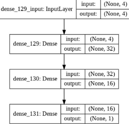
The architecture of the first feature extractor as shown in figure 4 has three layers in total.

(25)

Network 2:

In this network, "linear" activation function was used for the hidden layers and "relu" as the output activation function where the "linear" is represented by the equation (2) mentioned below:

φ(z) =z (2)

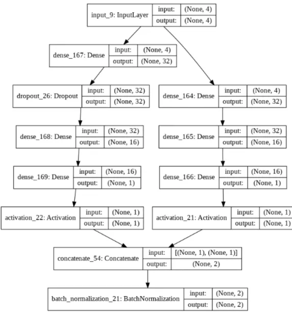
The architecture of the second feature extractor as shown in figure 5 has four number of layers in total including a drop out layer to randomly remove the nodes. Dropout probability of 0.5 was used.

Figure 5: Second Feature Extractor

The activation function "relu" where it was used in both networks as an output activation function is represented by the equation (3) below:

(26)

Measuring Heterogeneity of Individual Feature Extractors

The heterogeneous or diverse nature of the the members of a team of classifiers is considered to be an important aspect when combining various classification models. If the combined classifiers are of similar nature then the ensemble approach does not seem to be valuable. In order to ensure the diversity of the classifiers, it is a good approach to measure the diversity between the classifiers in some way. However, there is no concrete way or an accepted formal definition to measure the diversity between the classifiers. We measure the heterogeneity of our individual feature extractors on the basis of their output predic-tions. We make use of some parameters mentioned in [26] which can

be helpful for us to determine the diversity in predictions made my each classifier.

The parameters that we use require the number of correct and wrong predictions from both the classifiers as mentioned in 2below:

Table 2: Individual Feature Extractors Predictions

FE 2 [ correct (1) ] FE 2 [ wrong (0) ] FE 1 [ correct (1) ] N11 N10

FE 1 [ wrong (0) ] N01 N00

The parameters which we use are mentioned below: • Q-statistics:

The value range of Q-statistics parameter is between -1 and 1. In case of statistically independent classifiers, the expectation of Q-statistics is 0. Classifiers that tend to recognize the same objects correctly will result in a positive values of Q-statistics, whereas those committing errors on different instances will give out Q-statistics value as negative. The formula was Q-statistics is represented as:

Qi,k =

N11N00−N01N10

N11_N00₊_N01_N10 (4)

• The correlation co-efficient:

The correlation coefficient parameter here represents a statistical measure of the strength of the two classifiers. A negative value represents a negative correlation whereas a positive value shows a perfect positive correlation. It is represented by as:

ρi,k =

N11N00−N01N10 p

(N11₊_N10₎₍_N01₊_N00₎₍_N11₊_N01₎₍_N10₊_N00₎ (5)

• The disagreement measure:

(27)

the number of observations on which one classifier is correct and the other is incorrect to the total number of observations. The value range of this parameter lies between 0 and 1. It is represented by as:

Disi,k =

N01+N10

N11₊_N10₊_N01₊_N00 (6)

• The double-fault measure:

The double-fault measure is defined as the proportion of the cases that when observations have been wrongly classified by both classifiers. It is represented by as:

DFi,k =

N00

(28)

Ensembling of Feature Extractors:

The architecture of the ensembled feature extractor as shown in figure 6involves the concatenation of two individual feature extractors with a batch normalization layer.

(29)

Justification of Ensembled Network

After we created an ensembled network, the next step was to ensure that it is not just a larger version of the individual feature extractors. For this purpose, we modified our individual feature extractors by making the following changes one at a time:

1. Doubling the number of layers.

2. Doubling the activation units while keeping the number of layers same.

A performance comparison of the modified individual feature ex-tractors and our created ensemble network was done and is shown in result chapter5. Results from both individual networks are mentioned in tables7and8for feature extractor 1 and 2 respectively.

(30)

3.3 complete network architecture 24

3.3 c o m p l e t e n e t w o r k a r c h i t e c t u r e

Here, we show the complete architecture of our work and mention the parameters as well. Our network includes a unique way of feature extraction approach in DANN using ensembling techniques and is capable of giving improved performance. The hyper-parameters for the feature extraction part have already been explained in the previ-ous section. The hyper-parameters of the remaining two components which are label predictor and domain discriminator are as mentioned below:

Label Predictor (hyper-parameters)

There are in total of two dense layers along with one batch-normalization layer present in label predictor architecture. The input activation func-tion is ’relu’ and the output activafunc-tion used is ’sigmoid’.

Domain Discriminator (hyper-parameters)

The domain discriminator architecture includes two dense layers, one batch normalization layer and one drop-out layer having 0.25 as prob-ability. The activation function used in the hidden layer is ’elu’. The input activation function is ’tanh’ whereas the activation function used for the output is ’sigmoid’.

Where ’elu’ activation function is represented by the equation (8) mentioned below:

φ(z) =

(

α(ex−1), for z<0

z, for z≥0 (8)

and ’sigmoid’ output activation function which is used in both, label predictor and domain discriminator is represented by the equation (9) mentioned below:

φ(z) = 1

1+e−z (9)

General Parameters:

The number of iterations/epochs used are 5000. The optimizer used is ’sgd’ and loss function as ’categorical crossentropy’. The batch size was set as 32.

(31)

3.3 complete network architecture 25

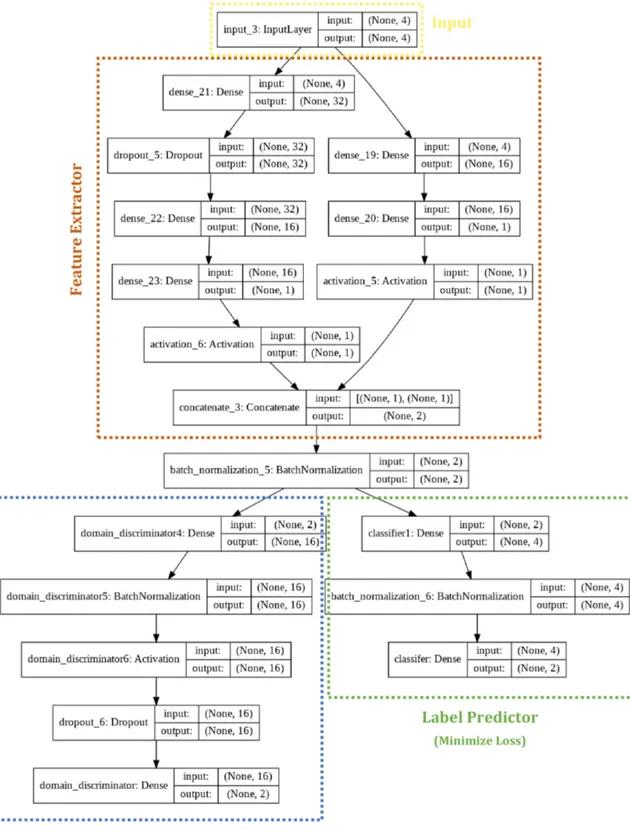
Our Proposed Network architecture is shown in figure7below:

(32)

3.4 transfer learning scenario/approach: 26

3.4 t r a n s f e r l e a r n i n g s c e na r i o/approach:

For transfer learning, the source domain(Xs), which is the training set

and the target domain(Xt), which is the test set are different due to

different operating conditions. In order to implement transfer learning, we created the following two scenarios:

• Single-to-Multiple / Multiple-to-Single Domain

For this scenario, we opted for leave out method approach. The model was trained on a specific air pressure value, considering it as source domain(Xs)and was tested on a range of different air

pressure values considering those as target domains(Xt). This

is the case of "Single-to-Multiple Domains".

– Source Domain(Xs):

Xs ={XA P=0.6} ; Ys={YA P=0.6}

– Target Domains(Xt):

Xt={XA P=0.1, ..., XA P=0.5} ; Yt={YA P=0.1, ..., YA P=0.5}

Later, the same procedure was repeated by swapping the source domain (Xs) and target domains (Xt) to make the case of

"Multiple-to-Single Domain". – Source Domain(Xs): Xs={XA P=0.1, ..., XA P=0.5} ; Ys={YA P=0.1, ..., YA P=0.5} – Target Domains(Xt): Xt ={XA P=0.6} ; Yt ={YA P=0.6} • Single-to-Single Domain

For this scenario, the source domain(Xs)is set to one specific

operating air pressure and the target domain(Xt)becomes all

other operating air pressures, but one at a time in a pair-wise manner. – Source Domain: Xs ={XA P=n} ; Ys={YA P=n} – Target Domain: Xt ={XA P=m} ; Yt ={YA P=m} Where; AP= {0.1, 0.2, 0.3, 0.4, 0.5, 0.6 } n∈ AP and m∈ AP ; f or n 6=m

We have implemented the above mentioned scenario for all air pressure values, which results a total of six cases of the Single-to-Single Domain Transfer.

(33)

4

S Y S T E M I M P L E M E N TAT I O N

4.1 p n e u m at i c s y s t e m d e s c r i p t i o n

The picture shown in figure8depicts how the pneumatic system by HMS looks like.

Figure 8: Pneumatic Reference System

The pneumatic system by HMS consists of multiple components including:

• Controlling System:

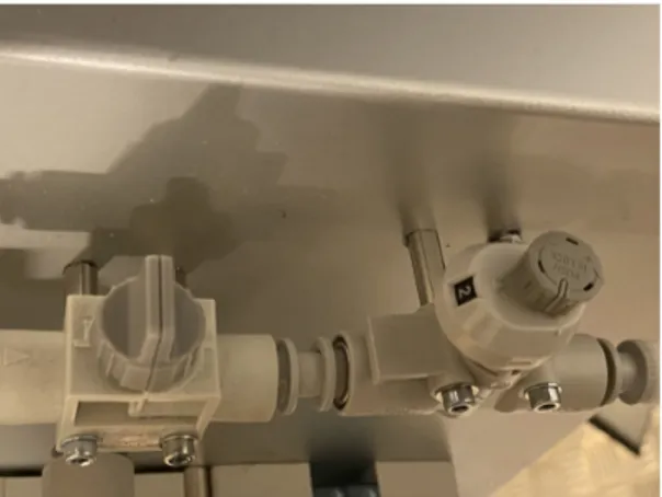
It is shown in figure9, which is responsible to control the two pneumatic system actuators (piston rods) using compressed air through tubes.

Figure 9: Controlling System

(34)

4.1 pneumatic system description 28

• Air Pressure Sensor (ISE40A-01):

This sensor in figure10, monitors base air pressure value within the pneumatic system in MPa unit. The air pressure readings can vary from 0 to 0.667 [21].

Figure 10: Air Pressure Sensor

• Air Flow sensor (PFMB7501-f04-f):

This sensor in figure 11, reads value about the airflow of the compressed air system in L/min unit. In addition to that, the associated accurately rated airflow ranges from 5 to 500 l/min [20].

(35)

4.1 pneumatic system description 29

• Pressure Valve:

it is used to adjust the base pressure level of the compressed air system. In other words, this value is used to change the operating conditions (range of 0.1 to 0.667)

• Actuators:

There are 2x Pneumatic piston actuators (rods) used to simulate an application and controlled by the pneumatic controller • Leakage valve/knob:

This leakage valve was used to simulate the air leakage in the pneumatic system. The system with leakage valve turned on is categorized as a faulty system.

• Regulator valve:

This regulator value shown in figure 12is used to control the amount or level of air leakage value induced in the system. It varies in a range from 0 till 11.

(36)

4.2 data collection settings / procedure 30

4.2 d ata c o l l e c t i o n s e t t i n g s / procedure

The sensor data can be sent on a software Sa.Engine, which is a Data Stream Management System (DSMS). In the first scenario, we collected the sensor data from Sa.Engine when there was no air leak in the pneu-matic system.Later in the second scenario, we simulated different amounts of air leaks in the pneumatic system and collected the data from the data stream management system (DSMS). The data collection experiments were varied by changing the base air pressure value to change operating air pressure, leakage knob to induce air leak and regulator valve level to vary the amount of air leak. As the data is multivariate time series data, so we can represent it as:

XA P ={x1t, x2t, x3t} ∈R ; YA P ={yt} ∈R

• Healthy Data:

The data collection for healthy data was collected at different air pressure values starting from 0.1 M/Pa to 0.6 M/Pa with a step size of 0.1MPa. The leakage value/knob was kept off to simulate no leakage in the pneumatic system.

XH ={XA P=0.1, ..., XA P=0.6} ; YH ={0}

• Faulty Data:

The data was collected at different air pressure values starting from 0.1MPa to 0.6 MPa with a step size of 0.1MPa. For every air pressure value, air leakage was induced by keeping the leakage knob on. The amount or level of air leakage was also varied by changing the regulator value. The starting value of regulator value was 1 and it was increased till 11 with step size 2. (i.e. regulator value having levels 1, 3, 5, 7, 9, 11)

XF={XA P=0.1, ..., XA P=0.6} ; YF ={1}

The data collecting process has been made on the pneumatic system by recording the air pressure values, airflow values, timestamp as well as the state of the actuators/pistons. We col-lected the data in different operating conditions experiments for both healthy and faulty data. Also, Manual feature engineering was also done by adding few more useful columns that could describe the dataset well.

4.3 e x p l o r at o r y d ata a na ly s i s

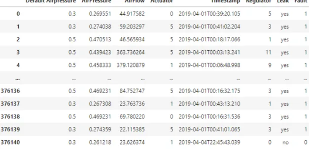
• Dataset:

This dataset shown in 13is generated by us through different experiments according to different operating conditions. Two types of datasets have been generated which are the healthy

(37)

4.3 exploratory data analysis 31

dataset (without inducing air leakage) and the faulty dataset (with air leakage) from the system.

X ={XH, XF} ; Y= {YH,YF}

where;

XH: Healthy Data Feature Space

YH: Healthy Data Labels

XF: Faulty Data Feature Space

YF: Faulty Data Labels

Both these datasets were combined to form the final dataset which looks as mentioned below containing approximately 360,000 rows and 8 columns.

(38)

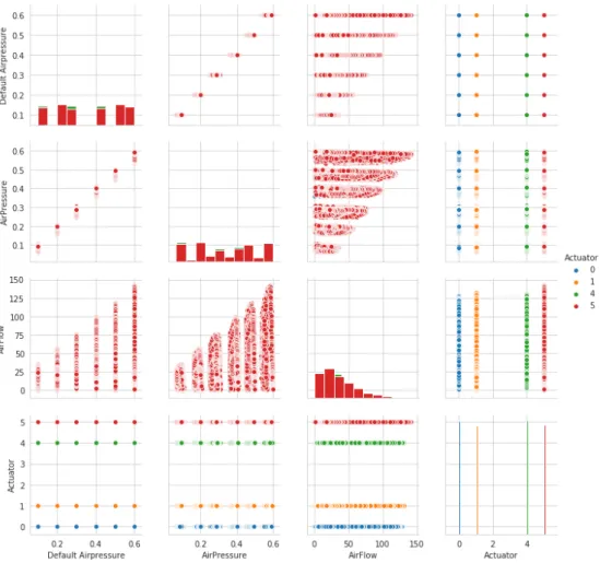
• Visualization

We initiated our work by visualizing the dataset and to find out the relationships between different features.

Firstly, we generated a scatter plot of the features of the healthy data (without air leakage) as shown in figure14to see the normal behaviour of the system.

Figure 14: Features Relationship (Healthy Data)

Later, we also plotted the scatter plot of features of the faulty data (with air leakage) as shown in figure 15 to find out the differences due to faulty condition of the pneumatic system. It was seen that the airflow values were increased as compared to the healthy condition.

(39)

Figure 15: Features Relationship (Un-healthy Data)

It can be seen from figure16as well that the airflow is increased in faulty state. For healthy state of the machine, the Airflow lies between 0-140 L/min whereas for unhealthy condition, the Airflow increases up to 480 L/min.

(40)

4.4 feature engineering and transformation: 34

4.4 f e at u r e e n g i n e e r i n g a n d t r a n s f o r m at i o n:

In all machine or deep learning algorithms, the input data known as features are required to produce outputs. The algorithms require features with some specific attributes or characteristics in order to perform properly and this arises the need of feature engineering. It involves producing a suitable feature from the existing features such that it can improve the prediction performance. It can include, arith-metic or aggregation operations on existing features to product a new one as a result of which the model can learn better than before [25].

We perform feature engineering or transformation with an aim to improve the learning of the model and give out better performance.

Thought behind generated feature:

It is a well-known property of the air that it flows from a region of high air pressure to low air pressure. In every pneumatic system, the air pressure is regulated at a higher pressure as compared to the room air pressure. In case of some air leakage, the air would leave out the pneumatic system with an increased air flow as compared to the normal operations of the pneumatic system. Also, we did some differences in the statistical information of the data with and without air leakage, as shown in Table3to understand the behaviour well. In the presence of air leakage, a higher value of air flow is seen and so is the standard deviation.

Table 3: AirFlow Statistics

Metric Healthy State Un-healthy State

Mean 27.79 L/min 140.27 L/min Standard Deviation 18.19 L/min 120.97 L/min Minimum 0.54 L/min 1.78 L/min

25% 12.77 L/min 46.15 L/min

50% 24.58 L/min 93.54 L/min

75% 38.73 L/min 212.77 L/min Maximum 86.67 L/min 445.19 L/min

Considering all this in mind, we came up with a new feature which could be applicable to all pneumatic systems and the formula for this feature is mentioned below:

F(new) = [( N

∑

i=1 AFni)/N] −AFXi (10)

(41)

where;

Fnew: Generated Feature

AFn: Airflow without leakage AFX: Airflow of particular instance

So, the first term in the equation is mean of airflow value when there is no air leak in the pneumatic system. These mean values are static for every air pressure which is then subtracted with air flow value of every instance.

This newly generated feature is generic and can be potentially useful for all pneumatic systems. It determines the deviation of the airflow from the mean of airflow when system has no leakage. In case of any leakage the variation becomes larger and turns out to be an anomaly. The condition to utilize this feature information requires presence of an airflow sensor/meter, which is likely to exist in most of the pneumatic systems.

In addition to that, we performed natural log transformation of AirFlow feature in which the data was skewed towards left. Reason behind log transformation was to have normal distribution of data for this feature. We can see the skewness and transformation of the feature in figure17mentioned below:

Air flow feature:

AirFlow_log=ln(AirFlow) (11)

(42)

Later, we generated a heat map as shown in figure 18to find out correlation with the target. Additionally, there are more methods to determine feature importance such as f-score, mutual information, recursive feature elimination etc. Also, we trained models using the original and transformed feature. Up to 1.5% increase in the accuracy performance was seen at the time of evaluation. The generated feature did not help when correlation was seen with the target which could be due to the sensors readings achieved as the rated flow range of the instrument is not so good. However, the log transformations of the feature was more useful than the original feature therefore it was opted for model training.

(43)

5

R E S U LT S

5.1 r e s u lt s e va l uat i o n c r i t e r i a

The performance of our proposed method will be evaluated as a classification problem relying on different metrics.

• Evaluation Metrics:

The diagnostics task is a classification problem which will be evaluated as mentioned below:

– Algorithm Performance: ∗ Accuracy ∗ Confusion Matrix ∗ Precision ∗ Recall ∗ F1-score

∗ Area under ROC ∗ Robustness [19]

– Generalization ability

It is good to evaluate the model with some more metrics rather than just seeing the accuracy. Performing evaluation by some additional metrics like precision, recall, f1-score can tell us about the performance on every output class. On the other hand, our method can also be evaluated by the company according to the computational performance analysis and cost-benefit analysis metrics [19]. This can give information about the feasibility of

the model for production state. • Model Comparison:

We compared our results with other machine learning and deep learning models.

• Model Testing:

We evaluated results on simulated data and can be done on some real data if provided by the industrial branch of the company.

(44)

5.2 experiments summary 38

5.2 e x p e r i m e n t s s u m m a r y

This section summarizes the following list of experiments that were performed and briefly explains the reason behind doing these experi-ments:

( I ) Machine/Deep Learning models vs Transfer learning model

This experiment was carried out to see how machine learning models and simple deep learning models would perform in a transfer learn-ing scenario. The main purpose of this experiment was to have some benchmark results and to demonstrate that the domain adaptation capability of our proposed network is beneficial in transfer learning scenario.

( II ) Selection/choice of Individual Feature Extractors

This experiment was performed as a justification for the choice of our individual feature extractors using which we form ensemble. In this experiment different number of layers and activation functions were tried (i.e. tanh, linear, relu, sigmoid) and then on the basis of performance, individual feature extractors were finalized.

( III ) Heterogeneity Measure between individual feature extractors

In this experiment we show the heterogeneous nature of our selected individual feature extractors. This was done by training the networks by substituting one individual feature extractor at a time in the feature extractor part and then analyzing their resulting output predictions from the label predictor part.

( IV ) Our proposed Network on leave-out method

This experiment was performed to depict the domain adaptation capa-bility of our proposed network in case of training on multiple domains and evaluating on a single domain (multiple-to-single). Additionally, there is another case in which training was done on single domain and evaluation was performed on multiple domains (single-to-multiple domains).

( V ) Performance comparison of individual feature extractors vs ensemble

This experiment is specific to our novel contribution in which we demonstrate the performance of our ensemble approach in compar-ison to the individual feature extractors. Our proposed network in-cludes an ensemble approach in the feature extractor part whereas a traditional domain adversarial neural network (DANN) possesses an individual feature extractor.

( VI ) Justification of Ensemble Network with enlarged individual feature extractors

This experiment was carried out with a purpose to justify that our ensemble is not just a bigger version of an individual feature extractor.

(45)

5.2 experiments summary 39

This was done by doing a performance comparison of our ensemble network with twice the size of individual feature extractors. The size of individual feature extractors was enlarged by either doubling the number of layers or the number of neurons.

( VII ) Our Proposed Network on single-to-single domain

This experiment was done to show the capability of domain adapta-tion of our proposed network when the model was trained on only one specific domain and was also evaluated on a single domain. We have created a 6x6 matrix to show the performance of our proposed network.

(46)

5.3 experimental results: 40

5.3 e x p e r i m e n ta l r e s u lt s:

( I ) Machine/Deep Learning models vs Transfer learning model:

For experimental results, we used leave-out method to create trans-fer learning scenario as mentioned inChapter 3. The modeling phase was divided into 4 stages:

• Applying Machine Learning Models:

We started by applying machine learning algorithms using Scikit-learn, machine learning library to observe the results. Also, hyper-parameters of all models were also fine-tuned using Grid-Search CV. It searches over specified parameter values for an estimator in an exhaustive manner. The parameters of the estima-tor used to apply these methods are optimized by cross-validated grid-search over a parameter grid.

Mentioned below machine learning algorithms were applied and Leave-out method was chosen for training purposes under transfer learning settings.

– Support Vector Machines (SVM):

Following were the best hyper-parameters for both cases and results are mentioned in figure19below:

CASE I:

[C=10, class_weight=None, degree=3, gamma=0.01, kernel=’rbf’, probability=True, random_state=None, verbose=False]

CASE II:

[C=10, class_weight=None, degree=3, gamma=’scale’, kernel=’linear’, probability=True, random_state=None, verbose=False]

(47)

– Logistic Regression:

CASE I:

[C=1, class_weight=None, fit_intercept=True, intercept_scaling=1, l1_ratio=None, max_iter=100, penalty=’l2’,solver=’liblinear’, ver-bose=0]

CASE II:

[C=10, class_weight=None, fit_intercept=True, intercept_scaling=1, l1_ratio=None, max_iter=100, penalty=’l2’,solver=’newton-cg’, verbose=0]

Figure 20: Logistic Regression [Left: Case I ; Right: Case II]

– Naive Bayes:

CASE I and II:

[priors=None, var_smoothing=1e-09]

(48)

– Random Forest:

CASE I:

[n_estimators=150, criterion=’gini’, class_weight=None, ran-dom_state=None, max_features=0.75 ,verbose=0, warm_start=False] CASE II:

[n_estimators=50, criterion=’gini’, class_weight=None, random_state=None, max_features=0.25, verbose=0, warm_start=False]

Figure 22: Random Forest [Left: Case I ; Right: Case II]

• Multi-layer Perceptron (MLP):

A simple multi-layer perceptron model was implemented using the Scikit-learn library. Following were the best hyper-parameters for both cases and results are mentioned in figure23 below: CASE I and II:

[activation=’tanh’, alpha=0.0001, epsilon=1e-08, hidden_layer_sizes=(50,), learning_rate= ’constant’, learning_rate_init=0.001, max_iter=200, momentum=0.9, shuffle=True, solver=’adam’]

(49)

• Correlation Alignment (CORAL):

CORAL (correlation alignment), a compact Python toolbox for transfer learning was also used which transformed the dataset. It is an unsupervised transfer learning technique that aligns the first and second-order statistics of the source and target data. CORAL minimizes domain shift by aligning the second-order statistics of source and target distributions, without requiring any target labels. [8] It is a domain adaptation technique that was

applied using MLP to observe the results. Following were the best hyper-parameters for both cases and results are mentioned in figure24below:

CASE I:

[activation=’tanh’, solver=’lbfgs’, alpha=0.0001, epsilon=1e-08, hid-den_layer_sizes=(50,), learning_rate=’constant’, learning_rate_init=0.001, max_iter=200, momentum=0.9]

CASE II:

[activation=’identity’, solver=’lbfgs’, alpha=0.0001, epsilon=1e-08, hid-den_layer_sizes=(50,), learning_rate=’constant’, learning_rate_init=0.001, max_iter=200, momentum=0.9]

(50)

Summary

So, we can see from the results in the figure25below that the machine learning algorithms as well as multi-layer perceptron (MLP) are not generalized due to no domain adaptation capa-bility. However, in the first scenario when Xs: 01.-0.5 and Xt: 0.6,

the algorithms are capable to perform good. Reason being that the target domain(Xt)is not that different and the learnt pattern

from basic algorithms can help. Whereas, in the second scenario where the difference is more between the domains, we clearly see that these algorithms miserably failed. We also observe one thing that correlation alignment (CORAL) performed better than all other algorithms due to basic transfer learning capability. We implemented correlation alignment (CORAL) in order to tell how transfer learning can have an impact when domains are different.

(51)

( II ) Selection/choice of Individual Feature Extractors

Here, we show the accuracy results for different network archi-tectures that we implemented in order to finalize the individual feature extractors using the "Grid Search" method. The final architecture was decided on the basis of accuracy results. Different number of layers and activation functions

We implemented different number of layers with different activa-tion funcactiva-tions (Grid Search) and computed the accuracy results as shown in Table4.

Table 4: Different Architectures with different Activation Functions

No of layers

Accuracy (%) Activation Function

tanh linear sigmoid relu

Case I Case II Case I Case II Case I Case II Case I Case II 1layer 84.73 76.91 86.06 83.27 86.12 82.70 87.05 81.83 2layers 86.92 82.81 82.36 80.21 83.62 83.52 86.06 82.16 3layers 87.16 84.94 86.79 81.73 80.97 82.66 86.19 78.73 4layers 84.61 81.36 87.33 84.44 79.92 83.56 86.59 75.62 5layers 84.19 83.07 86.92 83.51 80.64 81.50 86.85 74.83 6layers 86.26 79.20 86.06 83.36 80.11 77.32 86.98 70.24 7layers 87.12 74.83 86.92 82.60 74.60 72.86 83.91 72.36 8layers 82.29 75.88 86.39 84.04 74.27 73.02 84.21 70.97

The selected individual features are the ones which are high-lighted in table4and are chosen on the basis of highest accuracy results.