Evaluation of pipelines for analysis of next-generation sequencing data from CRISPR experiments

(1)

Bioinformatics-Research Project Advanced Level-30 ECTS

Autumn term 2019 Ansar Ahmad

b16ansah@student.his.se

Supervisor: Bjorn Olsson Examiner: Benjamin Ulfenborg

EVALUATION OF PIPELINES FOR

ANALYSIS OF NEXT-GENERATION

SEQUENCING DATA FROM CRISPR

EXPERIMENTS

(2)

ABBREVIATIONS

BAM binary alignment map

CRISPR Clustered Regularly Interspaced Short Palindromic Repeats DSBs Double Strand Breaks

FN False negative FP False positive

GEO Gene Expression Omnibus HDR homology-directed repair

NCBI National Center for Biotechnology Information NEAT NExt-generation sequencing Analysis Toolkit NGS next generation sequencing

NHEJ non-homologous end joining PCR Polymerase chain reaction PPV Positive predictive value

ROC Receiver operating characteristics sgRNA single guide RNA

SNP Short nucleotide polymorphism TN True negative

TP True positive VCF Variant call format

(5)

1. INTRODUCTION

1.1 Introduction:

The bacterial CRISPR (Clustered Regularly Interspaced Short Palindromic Repeats) system is the most robust and versatile genome editing technique to-date. Use of CRISPR for genome editing in eukaryotic cells was first reported in 2013 (Jinek et al., 2013) and is now widely used to execute targeted genome editing, enabling precise modification of genetic information in order to effectively study gene function, biological mechanisms, disease pathology and crop breeding (Cong et al., 2013). The CRISPR system replaced previously developed zinc finger nucleases (ZFNs) and transcription activator-like effector nucleases (TALENs) (Dahlem et al., 2012; Urnov et al., 2005), and was elucidated as an adaptive immune system for bacteria utilizing Cas enzymes complexed to RNA to identify invading virus and phage DNA (Barrangou et al., 2007). The system consists of a predesigned 20bp short guide RNA, for example the sgRNA (single guide RNA), and a custom-designed endonuclease like the Cas9 (Hsu et al., 2014). The sgRNA targets the endonuclease machinery to the genomic locus of choice containing the protospacer adjacent motif (PAM) and the site-specific endonuclease cleavage leads to DSBs (double strand breaks). The DSBs generated by Cas9 at approximately 3 bp upstream from PAM are subsequently repaired through either the cellular non-homologous end joining (NHEJ) or homology-directed repair (HDR) resulting in a wide range of outcomes including insertions, deletions, and nucleotide substitutions. In the case of HDR, recombination of extrachromosomal donor sequences is the resulting outcome (Canver et al., 2014; Mali et al., 2013; Ran, Hsu, Lin, et al., 2013; Ran, Hsu, Wright, et al., 2013).

Possible outcomes for a CRISPR/Cas9 genome editing in a single diploid cell include: no mutation, a heterozygous mutation where only one allele is mutated, a biallelic mutation where both alleles are mutated but the sequence of each allele is distinct or a homozygous mutation where both alleles carry the same mutation (Zischewski et al., 2017). The use of CRISPR/Cas9 for genome editing has been widely adopted in model organisms and systems such as mouse and zebrafish in previous researches (Hall et al., 2018; M. Li et al., 2016). Screening and characterizing the resulting mutations from CRISPR/Cas9 genomic edits in a large number of samples is made possible by next generation sequencing (NGS) which is

(6)

high-throughput, cost-effective and offers high-coverage and precise-quantification (Bell et al., 2014).

A big challenge in analyzing NGS data is how to handle the huge amounts of data and accurate detection of variants (Bianchi et al., 2016).To this end, many bioinformatic tools have been developed for NGS data analysis. These tools require significant work to install and to operate, and it is difficult to call mutations in NGS data and display results without an appropriate pipeline connecting different tools and automating the process. Pipeline tools are therefore becoming increasingly important for NGS data analysis and visualization of workflows. Using a pipeline to manage and run workflows comprised of multiple tools reduces workload and makes analysis results more reproducible (Ewels et al., 2016).

From a CRISPR/Cas-9 genome editing experiment and the subsequent screening of the outcome through NGS, variant calling follows. Variant calling is the process of identification of variants such as insertions/deletions (indels) and single nucleotide variants (SNVs). It is a multistep process with several potential error sources such as artifacts introduced during polymerized chain reaction (PCR) amplification, machine sequencing errors, base calling errors, incorrect local alignments of reads in the sequence data and challenges in deconvoluting mixed HDR/NHEJ outcomes, and these may lead to incorrect variant calls (Nielsen et al., 2011). Due to lack of validation data such as “gold standard” datasets or truth sets, pinpointing incorrect variant calls such as false positives and false negatives arising from these errors is significantly curtailed (Krusche et al., 2018). Experimental validation of all called sites across a whole genome can remedy this challenge by pinpointing incorrect calls, but this involves a lot of work and is quite costly. Due to these bottlenecks, accurate variant calling is a significant challenge in mutation screening in NGS data from a CRISPR/Cas-9 genome editing experiment (Altmann et al., 2012).

There are only a limited number of pipelines available for variant calling in CRISPR NGS data, and they all vary in their approach and use. Even though they all aim to call variants with high sensitivity and precision, many questions remain regarding how well they work in identifying and accurately calling sequence variation and estimating the true mutation efficiency (O’Rawe et al., 2013). Estimation of the true mutation efficiency and identification of candidate variants is dependent on multiple steps that are subject to different biases, and

(7)

methodological decisions for analyzing NGS data can significantly affect mutagenesis efficiency estimates (Lindsay et al., 2015). Following sequencing, reads have to be aligned to the correct reference, filtered for artifacts, and then the mutation efficiency has to be quantified and normalized. In many tools, many of the choices made during these steps are not clear to the user and may lead to potential misinterpretation of the data and widely different estimates of mutation efficiency (Labun et al., 2018). Comparing outputs from multiple tools and pipelines and learning from their methodological differences through evaluation studies can to some extent be an effective practical solution to minimize and prevent misinterpretation of the data analysis results.

There has been a limited number of CRISPR screening pipeline evaluation studies carried out to date (Roy et al., 2018). Lindsay et al. evaluated CrispRVariants against AmpliconDIVider, CRISPR-GA and CRISPResso (Lindsay et al., 2015). CRISPR/Cas9 experimental data (from pooled zebrafish embryos) was used to demonstrate CrispRVariants as the only CRISPR sequencing analysis tool that can adjust mutation efficiency estimates for existing genetic variation. In the synthetic simulated data mutation efficiency estimates of AmpliconDIVider, CRISPR-GA and CRISPResso’s were lower than those of CrispRVariants. Similarly, Labun et al. also evaluated ampliCan against CRISPResso, AmpliconDIVider and CrispRVariants in a benchmarking study (Labun et al., 2018). Their study also made use of both CRISPR/Cas9 experimental data from zebrafish embryos and synthetic simulated data where the synthetic data were used to quantify how much the different tools under evaluation differed in their mutation efficiency estimates. There were three synthetic datasets. In synthetic dataset 2, ampliCan matched the perfect score of CrispRVariants and AmpliconDivider. However, synthetic dataset 3 was slightly modified; it had adjusted length of amplicons and reads, its gRNA target sites were designed to be covered by both reads, PCR off-target reads were created without mutating the primer sequences, and mutation efficiency was tested across a range of mismatch rates (10%, 20% and 30%). In this synthetic dataset 3, ampliCan was more consistent at estimating mutation efficiencies within the dataset. CRISPResso performed poorly on all benchmarks. ampliCan obtained the highest precision and demonstrated the most robust performance when the mismatch rate of all bases was increased from 10% to 20% and 30%. Compared to other pipelines, ampliCan summarily displayed more consistency in the estimation of known indel efficiencies, identified large indels of >10 bp, and accounted

(8)

for the donor template and the original genomic sequence to define the set of events that corresponded to a correct HDR editing experiment.

False positive rates and false negative rates, as applied in the previous test study by Pinello et al. (Pinello et al., 2016), have also been used for assessment of the pipelines in this study. Using simulated data to assess the performance and limitations of CRISPResso, Pinello et al. observed that CRISPResso robustly and accurately identified editing events with a negligible false positive rate of not more than 0.1%. Altogether, their results indicated that CRISPResso was able recover the location and frequency of mutations with high accuracy and provided a reasonable estimate even in the absence of an untreated control sample.

CRISPRMatch (You et al., 2018) is a recently developed automatic stand-alone pipeline scripted in Python. It processes high-throughput CRISPR genome-editing NGS data by integrating analysis steps like mapping reads and normalizing read count, calculating mutation frequency, evaluating efficiency and accuracy of genome-editing, and visualizing the results in tables and figures. Its dependency packages include BWA (Burrows-Wheeler Aligner) (H. Li & Durbin, 2009), SAMtools (H. Li et al., 2009), Picard1_{, Pysam}2_{, and Matplotlibs (Hunter, 2007).}

CRISPRMatch was mainly developed for genome-editing data of CRISPR nuclease transformed protoplasts, which could evaluate the targeted mutation efficiency of DNA endonucleases and regions of guide RNAs quickly. It can analyze a series of CRISPR-Cas9 or CRISPR-Cpf1 NGS samples and compare the efficiency and accuracy of genome-editing endonucleases at one time. In the CRISPRMatch software test, its ability to analyze both Cas9 and CRISPR-Cpf1 NGS samples was tested using data from their previous work (Tang et al., 2017) and summaries of mutation frequency and details of genome-editing efficiency in each position was applied as an evaluation criterion for its robustness. In the test, CRISPRMatch identified different types of mutation - including deletion and insertion (Indels) - and the output was a set of charts, figures and tables on which the benefits and advantages of using CRISPRMatch such as expression, detailed mutation visualization, genome-editing efficiency evaluation and checking were assessed. CRISPRMatch has however currently not been previously benchmarked against any other commonly used NGS pipeline.

1_{https://broadinstitute.github.io/picard/} 2_{https://pypi.org/project/pysam/}

(9)

In this study project, a comparative evaluation of CRISPRMatch has been undertaken against the top-rated and commonly used CRISPR genome-edited NGS data analysis pipeline namely ampliCan (Labun et al., 2018) using simulated data as well as experimental CRISPR datasets deposited online in the BioProject database by Gagnon et al (Gagnon et al., 2014) under the accession number PRJNA245510 and experiments performed by Labun et al. (Labun et al., 2018) deposited online in ArrayExpress under accession numbers: 6310, E-MTAB-6355, E-MTAB-6356, E-MTAB-6357, E-MTAB-6358.

1.2 AIMS:

The aim of this study is to test two pipelines (ampliCan vs. CRISPRMatch) and evaluate their performance in terms of the ability to identify mutations correctly in CRISPR NGS data. In order to fulfill this aim, the following objectives will be pursued. The detection capabilities of NGS pipelines will be evaluated by:

• using simulated synthetic data to assess the true and false positives and negatives in datasets with known mutation values; and

• using experimental CRISPR datasets available from online databases such as ArrayExpress and BioProject.

The outcome and the analysis of this study will contribute to the limited number of CRISPR NGS data analysis pipeline validation studies and will potentially provide good insights for choosing a pipeline for CRISPR genome-editing NGS data analysis.

1.3 NGS data:

NCBI’s BioProject3_{provides a large collection of expression data. For this study, the}

experimental CRISPR datasets deposited online in the BioProject database by Gagnon et al (Gagnon et al., 2014) under the accession number PRJNA245510, and datasets in ArrayExpress under accession numbers: MTAB-6310, MTAB-6355, MTAB-6356, MTAB-6357, and E-MTAB-6358 have been utilized. Labun et al. (Labun et al., 2018) made use of this dataset in their study to benchmark and assess the performance of ampliCan against CrispRVariants,

(10)

CRISPResso and AmpliconDivider and showed that ampliCan is the most accurate and efficient of these three pipelines.

Synthetic NGS data has also been utilized in this study. The synthetic data has provided details on the variants present in the sets and their characterization such as read alignments and variant locations, and this has been used to assess the accuracy of the pipelines. In order to ensure the smooth operation of our assessment of these pipelines, synthetic data has been generated by the same technique as highlighted by Labun et al. (Labun et al., 2018). Their method utilizes an R script in the ART Illumina environment. The same method has been used in our experiments.

1.3.1 Methods:

The following two pipelines have been assessed and compared.

1.3.2 CRISPRMatch:

CRISPRMatch (You et al., 2018) is an automated toolkit developed to process high-throughput CRISPR genome-editing NGS data. It is scripted in Python. It integrates NGS read mapping, normalization of read counts, mutation frequency calculation, genome-editing efficiency statistics at each position of the target region, and results multiform expression. It maps and classifies reads, detects indels and calculates mutation frequencies, and outputs read alignment mutation details using BWA (H. Li & Durbin, 2009), SAMtools (H. Li et al., 2009), Picard4_{, Pysam}5_{and Matplotlibs (Hunter, 2007) dependency packages. CRISPRMatch takes}

target region sequence, sample information and sequencing data as input and outputs summaries of mutation frequency and details of genome-editing efficiency in each position through sets of charts, figures and tables in text and pdf formats. In its software test, CRISPRMatch for frequency calculation categorized three types of mutations as reads with deletion only, reads with insertion only, and reads with both deletion and insertion. Reads were categorized into deletion groups where deletions existed, insertion groups where insertions existed, and insertion and deletion group when both mutation types existed.

(11)

1.3.3 ampliCan:

ampliCan (Labun & Valen, 2018) is a comprehensive pipeline that determines the true mutation frequencies of CRISPR experiments from high-throughput DNA amplicon sequencing. It is implemented in R and Bioconductor, and uses the Needleman-Wunsch algorithm with tuned parameters to ensure optimal alignments of the reads to their loci. It quantifies the heterogeneity of reads, the complete mutation efficiency and the proportion of mutations resulting in a frameshift and also aggregates and quantifies mutation events of a specific type if a particular outcome is desired. ampliCan provides overviews of the impact of all filtering steps, and outputs. ampliCan takes in FASTQ files of sequenced reads and configuration files containing information about barcodes, gRNAs, forward and reverse primers, amplicons and paths to the corresponding FASTQ files. It then outputs reports containing plots summarized over all deletions, insertions and variants, reports summarizing the alignments of top reads, plots showing the general state of the experiments like heterogeneity of reads, and overviews of how many reads were filtered or assigned at each. Additionally, ampliCan produces R objects containing all alignments and read information, which can be manipulated, extended and visualized through the R statistical package. In its software test with synthetic datasets, ampliCan displayed more consistency in the estimation of known indel efficiencies compared to other pipelines. It was also able to identify large indels of >10 bp. It was also able to account for the donor template and the original genomic sequence to define the set of events that corresponded to a correct HDR editing experiment. ampliCan is compatible with most of the popular plotting packages, such as ggplot2 (Wickham, 2016) and ggbio (Yin et al., 2012), as well as the most popular data processing packages, such as dplyr (Wickham & François, 2015) and data.table.

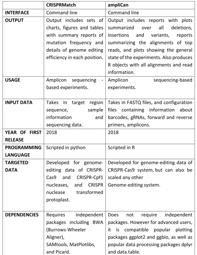
ampliCan can be used alone or integrated with the CHOPCHOP guide RNA (gRNA) design tool (Labun et al., 2016) to incorporate all computational steps necessary for a CRISPR experiment. Comparison of CRISPRMatch and ampliCan is presented in table 1.

(12)

CRISPRMatch ampliCan

INTERFACE Command line Command line

OUTPUT Output includes sets of

charts, figures and tables with summary reports of mutation frequency and details of genome editing efficiency in each position.

Output includes reports with plots summarized over all deletions, insertions and variants, reports summarizing the alignments of top reads, and plots showing the general state of the experiments. Also produces R objects with all alignments and read information.

USAGE Amplicon sequencing

-based experiments.

Amplicon sequencing-based experiments.

INPUT DATA Takes in target region

sequence, sample

information and

sequencing data.

Takes in FASTQ files, and configuration files containing information about barcodes, gRNAs, forward and reverse primers, amplicons. YEAR OF FIRST RELEASE 2018 2018 PROGRAMMING LANGUAGE

Scripted in python Scripted in R TARGETED

DATA

Developed for genome-editing data of CRISPR-Cas9 and CRISPR-Cpf1 nucleases, and CRISPR nuclease transformed protoplast.

Developed for genome-editing data of CRISPR-Cas9 system, but can also be scaled any other

Genome-editing system.

DEPENDENCIES Requires independent

packages including BWA (Burrows-Wheeler

Aligner),

SAMtools, MatPlotlibs, and Picard.

Does not require independent packages. However for advanced users, it is compatible popular plotting packages ggplot2 and ggbio, as well as popular data processing packages dplyr and data.table.

(13)

2 MATERIALS AND METHODS

2.1 Materials and Methods:

There are only a limited number of pipelines available for variant calling in CRISPR NGS data, and they all vary in their approach and use. Thus evaluation studies are important to assess the performance of the available pipelines, compare their outputs and learn from their methodological differences to minimize and prevent misinterpretation of the NGS data analysis results.

This study has evaluated the performance of the CRISPRMatch pipeline against the top-rated and commonly used pipeline namely ampliCan.

2.2 Datasets

BioProject is a public database maintained by the National Center for Biotechnology Information (NCBI). It provides a large collection of both raw and processed expression data as well as written experimental designs, sample attributes, and methodologies for studies (Clough & Barrett, 2016). To assess the performance of the aforementioned pipelines, experimental CRISPR datasets deposited online in the BioProject database by Gagnon et al. under the project ID PRJNA245510 were used. In their study, Gagnon et al. applied a detailed protocol that entailed target site selection, sgRNA production, stop codon cassette design, Cas9 protein purification and injection to generate these datasets using the TLAB strain of zebrafish as a model organism. In summary, Cas9 mRNA and sgRNA were co-injected into the zebrafish zygotes, and genomic DNA prepared. Polymerase chain reaction (PCR) was then used to attach barcoded sequencing adapters and to amplify approximately 120–300 base pairs of genomic sequence surrounding the targeted locus. The amplicons were later purified, pooled, and finally sequenced on a MiSeq to obtain paired-end reads (Gagnon et al., 2014). Labun et al. utilized this same dataset in their study to benchmark the performance of their pipeline ampliCan against CrispRVariants, CRISPResso and AmpliconDivider pipelines (Labun et al., 2018). It will be interesting to compare the results of ampliCan using the same dataset used by Labun for comparison with the newer pipeline CRISPRMatch.

In addition to the real experimental data, a simulated NGS dataset has also been utilized in this study. Generally, simulated datasets are functionally similar to sequencing output but

(14)

with all underlying mutations known. In most cases, accurate variant calling pipeline assessments are hindered by the lack of “ground truth” information about the variants present in the sequencing data. Therefore, simulated datasets significantly improve the accuracy of assessments of variant calling pipelines by characterizing the dataset to be used. Details available and known in simulated datasets include the variants present in the datasets, read alignments, read lengths and precise variant locations. Previous benchmark and test studies have also made use of synthetic simulated data. In the benchmarking study of CrispRVariants, Lindsay et al. applied a custom R script to generate a synthetic benchmark dataset (Lindsay et al., 2015). Labun et al. replicated the simulation strategy applied by Lindsay et al. and also applied the same custom R script to generate a synthetic dataset for their benchmark study of ampliCan (Labun et al., 2018).

Other, simulator toolkits are also publicly available, but they all differ in their error model (empirical or theoretical) used to generate synthetic datasets. Examples of such tools include ART (Huang et al., 2012), CuReSim (Caboche et al., 2014), GemSim (McElroy et al., 2012) and NEAT (Stephens et al., 2016) et cetera. ART simulates reads for the Illumina, 454 and SOLiD sequencing platforms and can define the number of reads to be produced per amplicon. CuReSim does not use an error model and its parameters must be specified on the command line. GemSim on the other hand uses an empirical error model to mimic individual sequencing runs and assumes a uniform or constant error rate for all positions within a sequencing read. NEAT provides the simulator software to generate reads as well as a set of scripts to extract many of the simulation parameters from real data (Stephens et al., 2016). However, these simulators are not adequately documented and can thus be difficult to use for non-experts. Generally, all these simulators can introduce different types of variants such as short nucleotide polymorphisms (SNPs), indels, inversions, translocations, copy-number variants etc. in the simulated sets (Escalona et al., 2016). All of this results in variability of synthetic data generated using inherently different simulator toolkits without adequate documentation and perhaps even without complete understanding of the functions resulting in variations introduced in the synthetic data analyzed.

Here, in order to induce some form of standardization between Labun, Lindsay, and the present study, it was decided to use the same R script method used by the other scientists to

(15)

generate synthetic data and conduct the analysis. An analysis conducted then would be more comparable with the other authors’ work.

The R script was designed by Lindsay et al. in 2016 to generate synthetic data of 20 genes (see supplementary note 10 for genes details) from Danio rerio (zebra fish) and was used to compare the performance (mutation detection) of CrispRVariants with other well-known CRISPR pipelines of that time. In 2018, the R script was again used by Labun et al. and then slightly modified for his study of comparison of ampliCan against other pipelines.

It uses danrer7.fa as reference genome file and generates synthetic data of 20 genes. It adds mutations in the form of insertions, deletions, indels, cuts and variants using mutation weight levels obtained from Shah et al. (Shah et al., 2015). This script runs under the ART_ILLUMINA environment and generates forward and reverse reads followed by merger to form paired end reads (300 bp). It generates the following percentage of mutation: 0%, 33%, 67% and 90%. It is also capable of generating varying amounts of deletions, insertions, cuts, and indels at four different frequencies namely 1, 2, 3 and 4. For greater details see supplementary note 11.

(16)

2.3 Variant Calling Pipelines

2.3.1 CRISPRMatch

CRISPRMatch is an automated pipeline most recently developed to process high-throughput CRISPR-Cas9 and CRISPR-Cpf1 genome-editing NGS data (You et al., 2018). Scripted in python, CRISPRMatch integrates NGS reads mapping, reads count normalization, mutation frequency calculation, genome-editing efficiency statistics at each position of target region, and outputs visualizations in the form of tables and figures. It maps and classifies reads, detects indels and calculates mutation frequencies, and outputs read alignment mutation details. With BWA (Li & Durbin, 2009), SAMtools (Li et al., 2009), Picard6_{, Pysam}7_{and Matplotlibs (Hunter, 2007)}

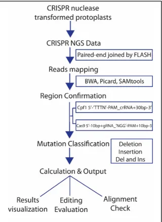
dependency packages, data processing, analysis and outputting are executed automatically. Paired-end reads are joined by FLASH (Magoč & Salzberg, 2011) to become single long reads and these are mapped to the target editing region by BWA software. The aligned files are then sorted and indexed by Picard and SAMtools, and the genome-editing

system types and target regions for mutation calculation are confirmed. Manual definition of the two cleavage regions of the endonucleases is also performed. The 5'-3' region from 10 base pairs upstream, gRNA, 'NGG' PAM, PAM, to 10 base pairs downstream is defined for Cas9. For Cpf1, the 5'-3' region covered 'TTTN' PAM, crRNA and 30 base pair downstream. The pysam package detects different types of mutations, including deletions and insertions that

Figure 1: Description of the steps involved in CRISPRMatch data processing. 1) A target gene index is built 2) deep sequencing reads are mapped by paired end sequencing read and joining into a single long read by FLASH 3) mutation detection namely insertion, deletion and combination indels is performed 4) efficiency calculation is conducted and results exported. Two cleavage regions of the endonucleases are defined resulting in the pipeline’s ability to detect and classify the actions of Cas9 vs CPF1.

(17)

may be present in each mapped read. Reads are categorized into deletion groups, insertion groups, and insertion and deletion groups. The matplotlib package plots summaries of mutation frequency and details of genome-editing efficiency in each position. CRISPRMatch thus takes the target region sequence, sample information, and sequencing data as input. It then outputs summaries of mutation frequency and details of genome-editing efficiency in each position through sets of charts, figures and tables in text and pdf formats (figure 1). The software is available for public usage on GitHub8_.

2.3.2 ampliCan

ampliCan (Labun & Valen, 2018) is an automated pipeline designed to determine the true mutation frequencies of CRISPR experiments from high-throughput DNA amplicon sequencing

8_{https://github.com/zhangtaolab/CRISPRMatch}

Figure 2: Overview of ampliCan (Labun et al., 2018). Takes fastq files and experiments discription as input and gives out put in form of html reports.

(18)

(for greater details see supplementary note 7). Scripted in R, it quantifies the heterogeneity of reads and the complete mutation efficiency, as well as the proportion of mutations resulting in a frameshift. It also aggregates and quantifies mutation events of a specific type if a particular outcome is desired. Furthermore, it also provides overviews of the impact of all filtering steps and outputs. ampliCan takes in reads in fastq format, configuration files with barcodes, gRNAs, amplicons, forward and reverse primers information, and paths to the corresponding Fastq files. It then filters low quality reads either based on user settings or recognizing ambiguous nucleotides by default and assigns them to the particular experiment by searching for matching primers. From here, ampliCan implements the Needleman-Wunsch algorithm with tuned parameters to ensure optimal alignments of the reads to their loci and models the number of indels and mismatches to ensure that the reads originated from the particular loci. Primer dimer reads and sequences that contain a high number of indels or mismatch events compared to the remainder of the reads are filtered out, and mutation frequencies are finally calculated from the remaining reads using the frequency of indels that overlap a short region of up to 5bp around the expected cut site. The output includes reports containing plots summarizing overall deletions, insertions and variants, and the alignments of top reads. It also provides plots showing the general state of the experiments, such as heterogeneity of reads, and overviews of how many reads were assigned. ampliCan also outputs R objects containing all alignments and read information, which are manipulated, extended and visualized through the R statistical package (figure 2).

ampliCan is compatible with the most popular plotting packages ggplot2 (Wickham, 2016) and ggbio (Yin et al., 2012) as well as the most popular data processing packages dplyr (Wickham & François, 2015) and data.table. It can also be integrated with the CHOPCHOP guide RNA (gRNA) design tool (Labun et al., 2016) to incorporate all computational steps necessary for a CRISPR experiment.

The software is available for public usage on Bioconductor9_{or on Github}10_.

2.4 Evaluation Metrics

Mutation frequencies and mutation efficiency estimates have been used to assess the performance of the pipelines in this study. Mutation frequency is the total number of

9_{https://bioconductor.org/packages/ampliCan} 10_{https://github.com/valenlab/ampliCan}

(19)

mutations that exist and are known in a given dataset while mutation efficiency is the percentage of mutations identified by a particular pipeline, out of the total number of mutations that exist and are known in a given dataset.

Pinello et al (Pinello et al., 2016) compared the performance of CRISPResso against that of CRISPR-GA and showed that CRISPResso, even in the presence of sequencing errors, robustly and accurately recovered editing events with a negligible false positive rate of at or below 0.1%. Recently, Lindsay et al. (Lindsay et al., 2016) benchmarked CrispRVariants against CRISPResso, CRISPR-GA, CRISPRessoPooled and AmpliconDIVider under a range of scenarios. In this benchmarking study, Lindsay et al demonstrated that, given all the complexities and confounders, CrispRVariants performed better by giving a precise, transparent and reproducible pre-processing, providing easy visualizations of variant alleles across samples and allowing calculation of the mutation efficiency. Labun et al. (Labun et al., 2018) also most recently benchmarked ampliCan against other leading pipelines - CrispRVariants, AmpliconDIVider, CRISPResso and CRISPRessoPooled - and demonstrated that ampliCan outperformed the others in the face of common confounding factors. Both Lindsay et al. and Labun et al. applied the use of mutation frequencies and mutation efficiency estimates in their benchmarking studies (Labun et al., 2018; Lindsay et al., 2015).

In the current study, utilizing the synthetic data, false positives (FP), false negatives (FN), true positives (TP) and true negatives (TN) are calculated. From the observed FP, FN, TP and TN values positive predictive values (PPV) and sensitivity are also calculated and applied as additional metrics to evaluate the performance of the pipelines in this study. In summary, true positives are mutations identified by the pipeline being tested and are truly present in the synthetic simulated data, herein considered as the “truth set”. False positives are mutations identified by the pipeline being tested but are not truly present in the synthetic simulated data. True negatives are mutations that are not identified by the pipeline being tested and are not truly present in the synthetic simulated data. These are nucleotide bases that could not be a mutant form because of the parameters set by synthetic data generation where the original data file is assessed as “wild type”. False negatives are mutations that are not identified by the pipeline being tested but are truly present in the synthetic simulated data (Cornish & Guda, 2015). From these, PPV and sensitivity will be computed as follows;

(20)

PPV = TP / (TP + FP) Sensitivity = TP / (TP + FN)

It will be very interesting to verify the conclusions reached by the above highlighted test and benchmarking studies by applying all the above-mentioned performance evaluation metrics in this present evaluation study. The application of these metrics will be made possible using synthetic simulated data which will for the purpose of this study be considered as the “truth set”.

There are other metrics that have been applied in previous evaluation and benchmarking studies, such as precision-recall curves and the receiver operating characteristic (ROC) curves (Hwang et al., 2016). Precision-recall curves facilitate comparison of variant calling pipelines over the complete range of precision and sensitivity values and may be more informative than ROC curves (Jackson et al., 2017). However, as their computation will require installation and use of additional and quite complex software

such as hap.py11_{, these metrics will not be}

applied in this study.

2.5 Implementation:

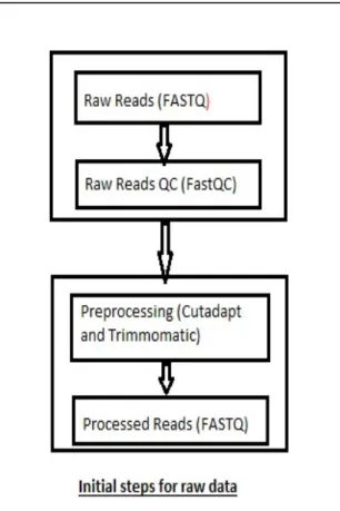
The initial datasets for zebrafish (Danio rerio), BioProject accession number PRJNA245510, were downloaded. This BioProject entry links to the SRA database where the read files are stored. The Ubuntu Linux version of the SRA-Toolkit was installed and used to download the read files SRR1264585 and SRR1264598 (run 1 and run 5 respectively), which are control samples from Gagnon’s data. (See supplementary note 1 for greater detail). These files contain 3,431,734 and 2,715,834 reads, respectively. The quality of the data was checked

11_{https://github.com/Illumina/hap.py}

Figure 3: representation of the steps for such experiments

(21)

using the FastQC program. After initial analysis, adapter trimming and paired end joining was performed with the aid of Trimomatic, cutadapt and fastq-join. A second FastQC analysis was performed prior to data analysis using ampliCan. See figure 3.

2.5.1 Obtaining Datasets:

The datasets used by Labun in his work, run 6 to 10 were downloaded manually from ArrayExpress (E-MTAB-6310, E-MTAB-6355, E-MTAB-6356, E-MTAB-6357, E-MTAB-6358).

2.5.2 Dataset Processing:

FastQC (by Babraham Bioinformatics), a software tool used to assess the quality of raw sequence data generated by high throughput sequencing pipelines, was utilized to ascertain the quality of data sets obtained from the SRA toolkit (linux version). (See supplementary note 2 for details).

(22)

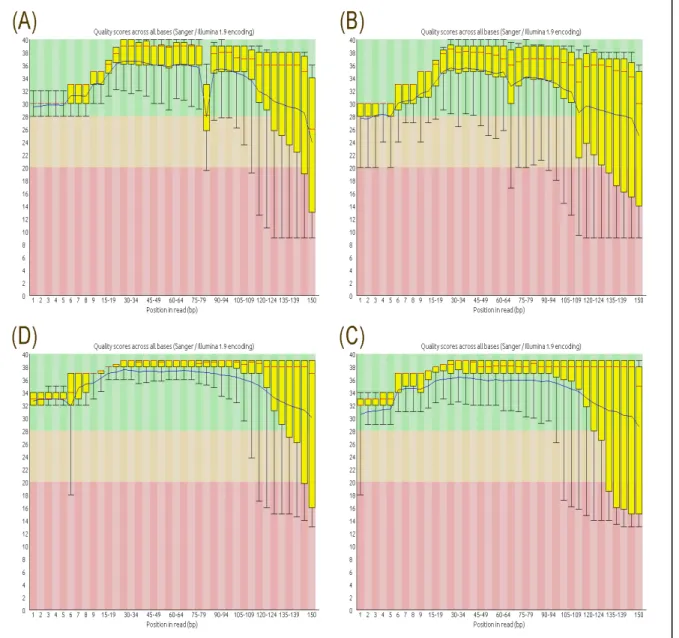
Figure 4: (A) quality score of raw dataset run 1 forward reads; (B) quality score of raw dataset run 1 reverse reads; (C) quality score of raw dataset run 5 forward reads; (D) quality score of raw dataset run 5 reverse reads. The central red line represents the median, yellow box represents the inter-quartile range, the upper and lower whiskers (error bars) represent the 10 and 90% points, and the blue line is indicative of the mean for each base pair’s position within the read (x axis). The y-axis shows the quality score with the background of the graph representing good quality data area as green, reasonable quality as orange and poor quality as red. Here, most of the data resides in the green area indicating good quality calls overall with some data falling in the red regions.

(23)

While the initial analysis of the data sets revealed acceptable sequence quality per base (Paired end data shown in Figure 4 (A) and (B)), a significant number of overrepresented sequences contributing to the increased size of the whiskers (increased error) in the FastQC were noted revealing a higher number of duplicated sequences including adapters. It was decided to remove the adapters to comply with research requirements. A list of adapters was obtained from Trimmomatic and after manually searching the data sets the cutadapt tool was

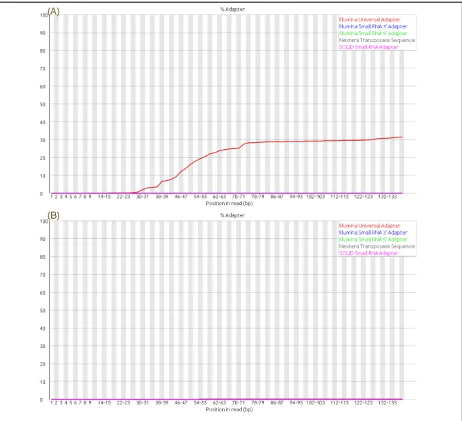
Figure 5: Cumulative plot of the fraction of reads where the sequence library adapter sequence is identified at the indicated base position. This can be used to identify adapters that are shorter than the read length resulting in read-through to the adapter at the 3’ end of the read. (A) adapter content in raw dataset run 5 reverse read prior to trimming while (B) shows adapter content after trimming in dataset run 5 reverse read indicating removal of over representative sequences. Similar analysis was conducted to similar results for run 1 as well. Representative data are shown here.

(24)

utilized on run 5 to generate research compliant data sets. (See supplementary note 3 for greater detail). Following adapter trimming, paired end joining (merging forward and reverse sequence into a single file) was performed utilizing the fastq-join tool (Aronesty, E., 2013) (See supplementary note 4 for greater details). A subsequent FastQC analysis of the adapter trimmed and paired end joined sequence was performed. The FastQC tool indicated the adapter content tab as green indicating the fitness of our data set for further processing (See supplementary note 5 for greater detail). The resulting data sets (paired-end images) are shown in Figures 5A and 5B.

2.5.3 ampliCan Pipelines Analysis:

After initial FastQC data analysis and adapter trimming followed by paired end joining, data quality was assessed and finalized using FastQC once more. The data were now considered ready for analysis using ampliCan. However, significant requirements for ampliCan analysis had to be satisfied. Following is a description of the method of data analysis using ampliCan. An R script was written to download all packages that are dependencies for the ampliCan pipeline (See supplementary note 6 for greater details). Additional software required by the pipeline was installed, including BWA (v 0.7.12) (Li & Durbin, 2010), seqprep, pear (v0.9.10), blat (version 35x1), CRISPResso (1.0.13), art_illumina (2.5.8) (See supplementary note 7 and the flow chart in graphical view of ampliCan shown in Figure 2).

2.5.4 Method:

After completion of installation and optimization of ampliCan, using a self coded R script, runs 1, 5 and 6 were analyzed (See supplementary note 8).

As per the requirements of ampliCan, a config.csv file containing information regarding forward and reverse primers, gRNA, amplicon sequence, and control etc. was created. The amplicon sequence was obtained from the UCSC genome website, guide RNA was obtained from the CHOPCHOP web-tool (Labun et al., 2016) (See supplementary note 8 for details on commands used for analysis in ampliCan). Once runs 1, 5, and 6 were analyzed using ampliCan, synthetic mutated datasets generated using the R script were also analyzed with ampliCan and are presented and discussed in the results section (Section 3 and Section 4).

(25)

2.5.5 CRISPRMatch pipeline Analysis:

Real data from Gagnon et al., run 1, run 5 and run 6, were then processed using CRISPRMatch. As an analysis tool, CRISPRMatch requires relatively fewer steps to setup and initiate processing. Its ability to communicate with both CRISPR dataset Cas9 and Cpf1 file types as well as its relatively few dependency packages make it a user-friendly tool for high-throughput CRISPR data analysis.

Subsequent to CRISPRMatch download and installation from github, the following dependency packages were installed: Anaconda, python3, bwa, samtools, picard, matplotlib, pandas, numpy, argparse and FLASH. (see figure 1 for CRISPRMatch analysis flow chart)

2.5.6 Methods:

Run 1, run 5 and run 6 were analyzed using CRISPRMatch by completing two main files. A reference FASTA file was also obtained for analysis using CRISPRMatch. (see supplementary note 9)

GuideRNA PAM with known start and end positions and an amplicon sequence was obtained like ampliCan analysis, though strand direction and start and end positions were manually provided. The samples to be compared as well as a control sample were also obtained. A synthetic dataset was then created to analyze the pipelines. (see supplementary note 11 for greater details)

2.5.7 Generating Synthetic Dataset:

For the purpose of benchmarking and comparing the pipelines, simulated datasets are needed so that it will be known which mutations were introduced. When the mutations detected by each pipeline can be compared to the known (artificially induced) mutations, it will be possible to calculate performance measures that can be compared between the pipelines. An R script used by Lindsay et al. (Lindsay et al., 2016) and Labun et al. (Labun et al., 2018) was used during this study as well, so that there will be a similarity and a standardization. For details on how synthetic datasets were generated, see supplementay section 11.

ART is a collection of simulation tools used to generate synthetic next generation sequencing reads. The R script utilized in this study runs under the ART_ILLUMINA toolkit environment and generates synthetic data. Here, synthetic data for 20 genes that are part of the original

(26)

experimental sequence file (danrer7.fa) of reference genome was utilized by the R script under the ART ILLUMINA toolkit environment to generate synthetic data. It adds mutations according to Shah et al.’s guide lines (Shah et al., 2015) in the form of deletions, insertions, cuts, variants and indels. These guidelines were established in 2015 and utilized by seqprep (St John, J. 2014) to merge the pair-end reads. The guidelines specified using 100% matched merged reads reduces sequencing error in analysis by removing all unpaired reads and collapsing the forward and reverse pairs into a single read followed by generation of XML files containing all the reads for a single amplicon.

(27)

3 Implementation and Results:

3.1 Results:

CRISPR is a family of DNA sequences that is found within bacterial and archaeal genomes. It is akin to a bacterial immune defense in which a DNA fragment of bacteriophage-derived sequences (from phages that previously infected the bacteria) are used to detect and destroy DNA from similar infections occurring subsequent to the original infection. Various endonucleases have been found to function with guide sequences to cleave the infecting DNA from bacteriophages. Among these, CRISPR-associated protein 9 (Cas9) and Cpf1 (CRISPR from Provetella and Francisella 1) now called Cas12a are of particular interest to researchers for use in introducing various forms of mutations in double stranded DNA (dsDNA). Cas9 is a 4 component system consisting of two small crRNA molecules and trans-activating CRISPR RNA (crRNA). These components have since been fused by scientists to generate a single guide RNA that functions with the endonucleases (Figure 6). The Cas9 endonuclease works downstream

of a protospacer adjacent motif (PAM) that needs to be G-rich while the Cpf1 endonuclease Figure 6: CRISPR endonucleases Cas9 and Cpf1. Cas9 (CRISPR associated protein 9) endonuclease functions with the aid of a guide RNA (gRNA) and requires the presence of a G rich PAM region. In a Cpf1 (CRISPR from Prevotella and Francicella 1), a T-rich region (TTTN) acts as a protospacer adjacent motif (PAM). It generates double stranded breaks (DSB) distal from the recognition site while Cas9 generates DSB’s proximal to the recognition site (three nucleotides away) and the resultant DNA has blunt ends. For both types of CRISPR endonucleases the DNA repair occurs by the nonhomologous end joining (NHE) and homology directed repair (HDR).

(28)

requires a T-Rich motif. The two endonucleases also function differently from each other in that Cas9 results in the generation of blunt end DNA while Cpf1 results in the generation of sticky ends of DNA.

Custom designed endonucleases can generate a large amount of DNA breaks and are an attractive avenue of research for the introduction of specific mutations. They are also capable of generating significant amounts of sequence data, requiring the need for specialized, high coverage, high throughput sequencing methods. Various pipelines have been developed and continue to be developed to perform these tasks. In simplest terms, an NGS pipeline should be able to accurately detect mutations with minimal to no errors. Previously, as shown by Labun et al. in 2018, ampliCan has been established as superior to the other known pipeline tools (CRISPResso, CrisprVariant, Amplicondivider). Here, we chose to study ampliCan against CRISPRMatch (a new pipeline with the advantage of being able to analyze data generated by Cpf1 as well as Cas9 endonucleases). Here, synthetic data generated using a method previously described by Labun et al was used to: 1) assess the user friendliness of both the processing and data output 2) compare the accuracy of mutation detection against the control sequence and 3) compare the detected mutation efficiency of CRISPRMatch to that detected by the current best as shown by Labun et al (ampliCan).

3.1.1 Synthetic data analysis using ampliCan:

An R script was used to generate synthetic data for multiple gene families (Neuroligin, Contactin associated protein, Neurexin, tight junction protein, and gap junction protein) (total 20 genes) (see supplementary note 10 for the description of the proteins tested). Among these, CNTNAP5 (Contactin associated protein AP5) is used as a representative of data synthesis and detection success. In the current study (as in the previous studies) any gene modified by the R script can be used to conduct the analysis as it is the mutation generation that is being tested and no single gene itself (for other genes see supplementary note 11). This R script has been used in the past by both Lindsay et al and Labun et al for their analysis and was thus chosen to maintain a standard of treatment for synthetic data generation. Figures 7-9 show the results of this analysis for 200 mutations frequency 2 (67% mutations inserted) (Figure 7-9). For other mutation levels analyzed by ampliCan as part of this analysis see supplementary note 11.

(29)

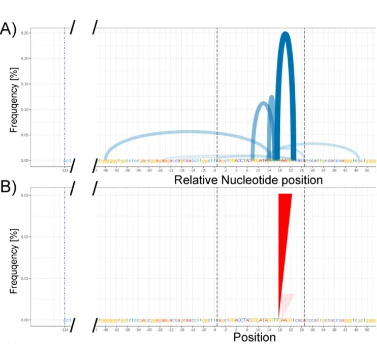
Figure 7: AmpliCan pipeline processed data for synthetic/generated data constrained to 200 mutations (67% mutations) within the sequence for CNTNAP5 (Contactin like protein AP5). (A) corresponds to a deletion plot produced by ampliCan for CNTNAP5 gene analysis and shows arches that represent deletions (x-axis, start to end of arch) present at a frequency indicated by the y axis and transparency. Verticle dotted lines represent the start and end of the primers. As the number of mutations grows in the synthetic data, the size of the deletions, insertions, and cuts increases accordingly and is detected by ampliCan (see supplementary figure 12-15 for the trend (B) corresponds to insertions (small amount of insertions detected).

(30)

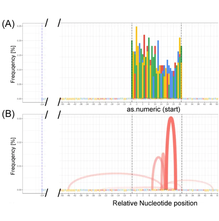
Figure 8: AmpliCan pipeline processed data for synthetic/generated data constrained to 200 mutations (67% mutations) within the sequence for CNTNAP5 (Contactin like protein AP5). (A) corresponds to Mismatches to the reference sequence (generated by R script during the earlier steps of the ampliCan processing) and (B) corresponds to cuts introduced to the sequence and whether they vary from traditional/PAM related cut sites. Arches represent cuts (x-axis, start to end of arch) present at a frequency indicated by the y axis and transparency.

(31)

Figure 9: The ampliCan pipeline processed data for synthetic/generated data constrained to 200 mutations (67% mutations) within the sequence for CNTNAP5 (Contactin like protein AP5). The figure shows an alignment plot in the 200 mutations data for the top 10 most abundant reads in a synthetic data experiment. Here the table on the right side of the figure shows the relative efficiency (Freq) of a read, the absolute number of reads (count). It also shows the summed size of the indels represented as F. A green color in F indicates a frameshift which is detected in this “200 mutation” dataset indicating that the ampliCan analysis is proceeding as expected. The percent match also indicates that the amount of sequence unmatched/mutated as generated in the synthetic data also matches the amount detected.

(32)

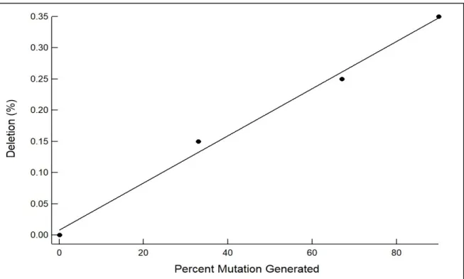
Figure 7 (A) exhibits the detected deletions as represented in the form of a deletion plot with arches. The two points of the arches connect the length of the deletion in the sequence (x-axis) and the transparency of the arch represents the number of times said cut was detected in the analyzed data (y-axis). The remaining data (for 0%, 33%, and 90% mutations can be found in supplementary note 11 figures 12-15). There, supplementary figure 12 (A) shows 0 cuts detected (as expected) since the R script did not introduce any mutations at this point. However, as the number of synthesized mutations increases in the synthetic data, the corresponding number of deletions and variation in the sizes of deletions increases. This suggests that ampliCan is able to detect the increasing number of deletions as introduced in the synthetic data. Looking at the y-axis for each image that shows frequency [%] in part A of Figure 7 as well as supplementary figures 13-15 we can see that the maximum height of the arch corresponds to a frequency [%] on the Y-axis. As you look at each image, it is obvious that the corresponding y-axis value is changing. This percent frequency of these deletions increases from 0.15 to 0.25 to 0.35 in the 33%,67% and 90% mutations datasets respectively. When you extract this information and plot it in a graphical software it can be fit to a linear model. The linear model fits this data well showing an R2 of 0.9926 for a slope of 0.0038 exhibiting near linear relationship between the increase in percent mutation introduced vs. detected (Figure 10). Assuming 90% mutations occurring in the samples corresponding to 90% mutations the

Figure 10: Percent mutations generated vs Percent deletion frequency plotted as a scatter plot and fit to a line with a slope of 0.0038 and an R2_{of 0.9926.}

(33)

calculated percentage of mutations in 33 and 67 % mutation samples is found to be 38.6 and 64.2% respectively. This is done by dividing the 0.15 percent frequency by 0.35 percent frequency and then multiplying it by 90 (percent normalization). This also indicates the presence of the correct number of deletions detected in the corresponding samples (See Table 2) when compared to the percent of mutations synthesized though indicates that most of the generated mutations are deletions while insertions and cuts play a less significant role in the R script used to generate synthetic data.

Part (B) of these supplementary figures (12-15) (see figure 7 B for 200/67% mutation) exhibits the insertions detected in the sequence during data synthesis. Interestingly, the data here do not change with changes in percent mutation though may account for the slight deviation from the near linear relationship of the deletions introduced as part of data synthesis. Understandably, the R script is supposed to introduce deletions as well as insertions and indels. As the majority of the mutations detected by ampliCan are deletions and not the other mutations introduced by the R script, the small variation of the deletions from a perfect linear fit could be because the remainder of the mutations are insertions and thus not part of the calculations conducted for deletions detection only. No insertions were detected by ampliCan in the 90% mutations synthetic dataset. Part (C) of the ampliCan supplementary figures (12-14) (see Figure 8 A for 200/67% mutation) and Part (B) of supplementary figure 15 represents the mismatches detected in the various regions within the sequence (colored in the same

Percent mutation generated Percent deletion frequency Calculated percent deletion 0 0 0 33 0.15 38.6 67 0.25 64.3 90 0.35 90

Table 2: Percent mutation generated vs. Deletion frequency output by AmpliCan vs. Calculated percent mutation derived using the assumption that maximum percent deletion frequency corresponds to 90%.

(34)

manner as the amplicon). In the current experiment, mismatches seem to have an inverse relationship, with the number of mutations generated going up and the frequency of mismatch going down. A similar relationship with deletions is also noticeable. Part (D) of supplementary figures 12-14 and Part (C) of supplementary figure 15 (see figure 8 B for 200/67% mutation) corresponds to cuts that occur during the data generation process, occupy the identical sequence and correspond to similar percent frequency (y-axis) indicating that the missing mutation total (i.e. Cuts) is mostly due to deletions.

The final part of supplementary figures 12-15 (Figure 9 for 200/67% mutation) contain an alignment plot for the corresponding percent mutation generated. In this part of each figure, the table on the right provides the relative frequency (Efficiency) of the read, the absolute number of reads (count), and the summed size of the indels (insertions and deletions) as F. Green color filled parts of the table correspond to a frameshift detected within each dataset. In the percent bar chart presented above the table on the right, the percent match indicates the percent of the sequence that matches the control sequence (pre-synthetic-mutation-generation). Here we can see that the synthesized data at 0 mutation, 33% mutation, 67% mutation, and 90 % mutation correspond with 100%, 67%, 33% and 10% match and corresponds well with the remaining un-mutated data. This shows that the synthetic data is detected by ampliCan with high efficiency and accuracy.

The R script affords users to assign the amount of variability withing the mutations inserted during the generation of the synthetic data. This is represented as increasing frequency of mutation addition to the sequence. A low “Freq” number corresponds to minimal/less drastic insertions, deletions and indels to the sequence while a larger number indicates greater variability. While the data shown in the results section and supplementary note 11 corresponds to CNTNAP5 and other various genes tested in the synthetic dataset at a mutation insertion frequency of 2, analysis was conducted (see supplementary results files provided) for other mutation frequencies as well. This data was analyzed for all 20 genes tested (supplementary note 11) and data regarding CNTNAP5 is presented here. This shows the variation in the data introduced due to the mutation insertion frequency value and can be

(35)

used to compare the relative efficiency of CRISPRMatch to the current standard (ampliCan) (Figure 11).

3.1.2 Synthetic Data Analysis using CRISPRMatch:

CRISPRMatch is a recently developed automatic stand-alone toolkit based on python script that has the ability to process the high-throughput, CRISPR nuclease dependent, genome editing data. It does so by integrating multiple analysis steps including mapping reads, normalizing read counts, evaluating the accuracy and efficiency of genome editing, calculating deletion and insertion frequency. In the final step of automated analysis, it generates visualizable results of the data (figures and tables). It also boasts the ability to analyze Cpf1 endonuclease generated sticky ends containing data.

The synthetic data generated by the R script and initially analyzed by AmpliCan was then analyzed using CRISPRMatch so that a comparison could be made between the two pipelines. Similar to the results for AmpliCan, CRISPRMatch analysis for CNTNAP5 is presented as part of the results section while representative genes of the CNTN, NLGN, NRXN families etc. are Figure 11: F (insertions and deletions) as detected by ampliCan Plotted against the increased number of mutations with 0, 100, 200, 270 corresponding to 0, 33%, 67%, and 90% respectively. This shows that an increase in frequency in the data synthesis process results in increased variation in the number of mutations synthesized with a frequency of four exhibiting the most significant variation in mutation numbers with increasing number of mutations added.

(36)

presented as part of the supplementary note 11 and the entirety of the analysis results are provided as supplementary files.

Data output in CRISPRMatch is presented in the form of bar charts. Figure 12 Part (A) and supplementary figure 22-24 part (A) represents the various forms of mutations detected in the sequence while part (B) of these figures is a representation of deletions within the samples. Part (A) of figure 13 and part (C) of supplementary figures 22-24 is a representation of deletion frequency and is hence directly comparable with deletion frequencies shown in the data visualization from top part. Figure 13 part (B) and supplementary figures 22-24 parts (D) could be considered as a non-visual representation of part (B) of these supplementary figures and of figure 12 which shows the control sequence against which the treatment is tested. This could also be compared to the alignment chart generated by AmpliCan (figure 9). Supplementary figures 22-24 show sequence analysis for 100, 200, 270 (33%, 67%, and 90%) synthetically generated mutation data. Supplementary figure 22 part (A) shows the distribution of all the various mutations present in the synthetic sequences. It detects mostly deletions and some minute quantities of insertions in this sample. With increasing number of mutations, CRISPRMatch continues to detect deletions and insertions in the sample with values ranging between 15%-40%. When these results are compared to the AmpliCan analysis they are found to be similar. Figure 12 B and 13 A show the frequency of deletion between the sample and control as well as deletion frequency of each sequencing sample respectively. The comparison between control and experiment are represented together as a qualitative representation of efficiency of genome editing experiments. In the ampliCan analysis, the same data is represented as the height of the arches indicating deletion frequency and the color intensity of the arch is indicative of the frequency of that deletion occurring in the same sample. The deletion frequency of the synthetic data detected by CRISPRMatch however, appears to be significantly higher than the one detected by AmpliCan. At 33% mutation level,

(37)

ampliCan detected a deletion frequency of 0.15 while CRISPRMatch detected a frequency of 0.30 (supplementary figure 22 Part (C).

Figure 12: CRISPRMatch output files for 200 mutation (67% mutation) data for CNTNAP5. (A) shows the bar chart that summarizes all-inclusive mutations (insertion, deletion, and combination of insertions and deletions) between “Treatment” (synthetic data) and “Control” unmutated data. The purple, orange and blue represent the frequency of all mutations, reads with deletion only, and reads with insertion and deletions respectively. If found insertion only data is represented with green bar. (B) is the summary of deletion among samples in a group and displays the frequency of deletion between the synthetically generated data and control.

(38)

Figure 13: CRISPRMatch output files for 200 mutation (67% mutation) data for CNTNAP5. (A) represents the deletion frequency of each sequencing sample where the x-axis shows the sequence of the genome and labels shown in red are parts of PAM. (B) shows the alignment profile of control showing mostly the same sequence represented on the top, while the bottom alignment exhibits the alignment result of partial reads (sample vs control) for the CNTNAP5 gene. Deletions are marked by – and the pattern of deletions corresponds to the histogram generated in (B).

(39)

The shape of the bar chart of deletion frequency in CRISPRMatch corresponds with the alignment data presented in the lower part of alignment in each figure representing CRISPRMatch data.

The trend of increased deletion frequency detection continues at the higher mutation level samples in supplementary figures 23 and 24-part C. The resulting curve (Figure 14) from compiling the deletion frequencies from the CRISPRMatch data (Table 3) fits to a linear fit extremely well (R2 of0.9991) but has a slope of 0.0088 which is greater than two times the slope of deletion frequencies obtained using ampliCan (Figure 15).

Figure 14: Percent mutations generated vs Percent deletion frequency plotted as a scatter plot and fit to a line with a slope of 0.0088 and an R2_{of 0.9991.}

90%.

Percent mutation generated

Percent deletion

frequency Calculated percent deletion

0 0 0

33 0.301 34.3

67 0.61 69.5

90 0.79 90

Table 3: Percent mutation generated vs. Deletion frequency output by CRISPRMatch vs. Calculated percent mutation derived using the assumption that maximum percent deletion frequency corresponds to 90%.

(40)

In all cases the deletions shown by CRISPRMatch are increasing in percentage in the same manner as ampliCan with the increase in the mutation level. Interestingly, though CRISPRMatch seems to be detecting more deletions, whether these deletions are truly present in the synthetic data remains to be seen. A comparison with true deletion in the sequence, manually detected, is presented in the later part of this report.

3.1.3 Analysis of Real Experiments using ampliCan and CRISPRMatch:

The investigation into next generation sequencing techniques was then extended into understanding how these two pipelines/toolkits may deal with real data rather than synthetically generated data. In order to do this, real experiment data was acquired from ArrayExpress as outlined by Labun et al (Run 6). Multiple genes were tested within this data analysis. Among those tested, the data of a representative gene, PITX2, is presented here. For remaining gene data see supplementary note 12. The real experiment dataset (263 real CRISPR experiments) was created by Labun et al where they combined 151 experiments that they had previously published (available at BioProject under accession number PRJNA245510), and 112 novel experiments from five sets for their most recent study (ArrayExpress: E-MTAB 6310, 6355, 6356, 6357, 6358). These experiments were conducted by

Figure 15: Percent mutations generated vs Deletion (%) plotted as a scatter plot for CRISPRMatch (CM, blue) vs ampliCan (AC, red) showing a slope of >2x when CM is used for detection of deletion within the synthetic sequences generated the R script.

(41)

injecting zebrafish zygotes which were sequenced two days after fertilization. Due to the rapid cell division within the early phase post-fertilization, these experiments most likely contain heterogeneous mutational efficiencies due to mosaicism. Thus, the true mutation efficiency is unknown and only a quantification of differences between the two tools could be presented here.

While during the synthetic data analysis, both CRISPRMatch and ampliCan showed similar trends (even though they ended up having dissimilar slopes for deletion frequency) in mutation detection, in the real experiment data, these trends are no longer present. Here, the ampliCan data shows significant number of insertions while the CRISPRMatch data indicates no insertions at all. As a comparative NGS sequence pipeline, CRISPRMatch should at least be able to detect some insertions. The fact that it is unable to find any insertions at all in data that by virtue of being real experiment data where one cannot control for zero insertions clearly speaks to CRISPRMatch being an inferior NGS pipeline to ampliCan. As endonucleases function in real experiments they are incapable of generating deletion only data. Thus any detection by an NGS pipeline in a real experiment that show zero insertions is erroneous and indicates a flaw in the pipeline itself. In deletion frequency comparison between the two pipeline both detected the same percent deletions at 0.04%.

(42)

Figure 16: AmpliCan pipeline processed data for real experimental data within the sequence for PITX2. (A) corresponds to a deletion plot produced by ampliCan for PITX2 gene analysis and shows arches that represent deletions (x-axis, start to end of arch) present at a frequency indicated by the y axis and transparency, respectively. Verticle dotted lines represent the start and end of the primers. Deletions of varying sizes and number are present. (B) corresponds to insertions. (Significant number of insertions detected in the sequence in question indicative of insertions during repair after double stranded DNA breaks caused by the endonuclease).

(43)

Figure 17: AmpliCan pipeline processed data for real experimental data within the sequence for PITX2. (A) corresponds to Mismatches to the reference sequence and (B) corresponds to cuts introduced in the sequence and whether they vary from traditional/PAM related cut sites.

(44)

Figure 18: AmpliCan pipeline processed data for real experimental data within the sequence for PITX2. The panel shows an alignment plot to PITX2 from uninjected sample showing about 65% match between the two. Here the table on the right side of the figure shows the relative efficiency (Freq) of read, the absolute number of reads (count). It also shows the summed size of the indels represented as F. A green color in F indicates a frameshift which is detected in the dataset.

(45)

Figure 19: CRISPRMatch output files for real experiment data for PITX2. (A) shows the bar chart that summarizes all-inclusive mutations (insertion, deletion, and combination of insertion and deletion) between “Treatment” (injected) and “Control” (un-injected) sample’s sequence for PITX2. The purple, orange and blue represent the frequency of all mutations, reads with deletion only, and reads with insertion and deletions, respectively. If found, insertion only data is represented with green bar. (B) is the summary of deletion among samples in a group and displays the frequency of deletion between the injected and un-injected sample data. (C) represents the deletion frequency of each sequencing sample where the x-axis shows the sequence of the genome and labels shown in red are parts of PAM. (D) shows the alignment profile of control shows sequence of control on left and treatment on right for the PITX2 gene. Deletions are marked by + – while the pattern of deletions does not correspond to the histogram generated in (B).

(46)

The biggest difference is notable between the alignment plots of the two methods. Here, ampliCan (Figure 18) shows 65% match and areas of frameshift mutations and deletions, while the CRISPRMatch result (Figure 19 part D) shows two alignment plots (un-injected vs. injected) that have minimal deletions within them, although the rest of the figure shows deletions etc.

Figure 20: CRISPRMatch output files for real experiment data for PITX2. (A) represents the deletion frequency of each sequencing sample where the x-axis shows the sequence of the genome and labels shown in red are parts of PAM. (B) shows the alignment profile of control, showing sequence of control on the left and treatment on the right for the PITX2 gene. Deletions are marked by – while the pattern of deletions does not correspond to the histogram generated in (B).