Accurate and Interpretable Regression Trees using Oracle Coaching

Accurate and Interpretable Regression Trees

using Oracle Coaching

Ulf Johansson, Cecilia Sönströd, Rikard König

University of Borås, Sweden

Email: {ulf.johansson, cecilia.sonstrod, rikard.konig}@hb.se

Abstract—In many real-world scenarios, predictive models need to be interpretable, thus ruling out many machine learning techniques known to produce very accurate models, e.g., neural networks, support vector machines and all ensemble schemes. Most often, tree models or rule sets are used instead, typically resulting in significantly lower predictive performance. The over-all purpose of oracle coaching is to reduce this accuracy vs. comprehensibility trade-off by producing interpretable models optimized for the specific production set at hand. The method requires production set inputs to be present when generating the predictive model, a demand fulfilled in most, but not all, predic-tive modeling scenarios. In oracle coaching, a highly accurate, but opaque, model is first induced from the training data. This model (“the oracle”) is then used to label both the training instances and the production instances. Finally, interpretable models are trained using different combinations of the resulting data sets. In this paper, the oracle coaching produces regression trees, using neural networks and random forests as oracles. The experiments, using 32 publicly available data sets, show that the oracle coaching leads to significantly improved predictive performance, compared to standard induction. In addition, it is also shown that a highly accurate opaque model can be successfully used as a pre-processing step to reduce the noise typically present in data, even in situations where production inputs are not available. In fact, just augmenting or replacing training data with another copy of the training set, but with the predictions from the opaque model as targets, produced significantly more accurate and/or more compact regression trees.

Keywords—Oracle coaching, Regression trees, Predictive mod-eling, Interpretable models

I. INTRODUCTION.

The purpose of predictive modeling is to obtain a model that produces accurate predictions regarding some phe-nomenon, typically described in terms of attributes and a target concept. When viewed as a data mining problem, this entails finding and modeling patterns between an input, in the form of an attribute vector, and an output, in the form of a single target variable. When the target variable is real-valued, the task is a regression problem, while target values from a set of predefined labels result in a classification task. Both prob-lem types have been extensively studied in machine learning and a wealth of techniques exist that produce models with good predictive performance. Generally, the best predictive

This work was supported by the Swedish Foundation for Strategic Research through the project High-Performance Data Mining for Drug Effect Detection (IIS11-0053), the Swedish Retail and Wholesale Development Council through the project Innovative Business Intelligence Tools (2013:5) and the Knowledge Foundation through the project Big Data Analytics by Online Ensemble Learning (20120192).

performance is obtained using techniques that produce opaque models, such as artificial neural networks (ANNs), support vector machines (SVMs) or ensemble techniques, where it is not possible for a human to inspect the relationships found by the model. When predictive accuracy is the only property of interest, this is perfectly acceptable, but in many applications interpretable models are needed, making it necessary for techniques to produce transparent, rather than opaque, models. In a transparent model, relationships between input and output are made explicit in some easily interpretable representation and hence allow insights into the underlying domain to be gained. Generally, this possibility comes at the price of reduced predictive performance, compared to an opaque model. The situation where predictive performance is sacrificed in order to obtain an interpretable model is known as the accuracy vs.

comprehensibility trade-off and has been discussed extensively

in data mining research, see e.g., [1, 2]. Apart from the obvious situation where a model needs to be interpretable in order for its predictions to be verified for legal or safety reasons [3], it has been argued that interpretable models increase user acceptance, see e.g., [4, 5]. It is important to note that a transparent model is not necessarily interpretable viewed as an entity, due to it possibly containing hundreds or thousands of symbols. However, in a transparent model it is, in principle, always possible to follow the logic behind each and every prediction made.

Experimental evaluation of machine learning techniques always includes reporting performance on data not used to train the model. Usually, a fixed amount of data with known target values is available, and has to be used both to train and evaluate the model. In this situation, all results regarding predictive performance carry the assumption that the data used to evaluate the model has not been used at all during model building and parameter tuning. However, it is important to realize that this is a situation that is not typical for real-world applications. Instead, the usual state of affairs is that historical data with known target values are available to build a data mining model that will be applied to some production data with unknown target values, in order to solve a business problem. In these cases, the only thing that really matters is maximizing predic-tive accuracy on this production data. A key insight here is that often a large number of production instances will be available, and the predictive model is actually built especially for these instances. Examples of applications where this might occur are when selecting recipients of a mass marketing campaign from a customer register or deciding which are the most promising compounds from a newly synthesized molecule library to further investigate during drug development. It should also be

noted that in many such instances, an interpretable model is desirable, or even mandatory.

We have previously suggested an approach called oracle coaching, especially aimed at increasing predictive perfor-mance on production data for transparent models. The idea is to build the transparent model in three steps:

1) build a high-performance opaque model using normal

training data, i.e., the available labeled data

2) employ the opaque model to obtain predicted target

values for both training and production instances

3) utilize the predicted values as training data for the

transparent model, possibly in conjunction with the original training data

The term oracle coaching comes from the underlying idea of viewing the stronger opaque model as an oracle, whose predicted values are regarded as true values by the transparent model during training. So far, studies using oracle coaching have only been performed on classification problems, but since the setup only relies on the availability of high-performance opaque models to serve as oracles and ditto transparent models to utilize the oracle data, it is natural to extend the concept to regression problems. The main contribution of this paper is thus the novel application of the oracle coaching for regression tasks, using readily available state-of-the-art techniques, in or-der to obtain increased predictive performance for interpretable models.

II. BACKGROUND.

The most commonly used representation for transparent models is decision trees, and particularly for classification, these are almost ubiquitously used when interpretability is needed. However, as pointed out by Dobra and Gehrke in [6], even though regression is an important task in data mining, regression trees have not been extensively studied, with the notable exception of Breiman’s CART [7] algorithm. They also note an increased interest in accurate and interpretable models for regression tasks. Despite this, more than a decade later, very few machine learning techniques aimed at producing interpretable regression models exist; with rule learning for regression, in particular, being an under-developed field [8].

Other than statistical methods, like (multiple) linear regres-sion, the most popular data mining techniques used to produce high-performance models for regression problems are ANNs and SVMs. Both these types of models have repeatedly been shown to obtain robustly good predictive performance in a wide range of applications, despite both being rather sensitive to parameter settings. Naturally, given any technique producing regression models, it is also possible to build an ensemble predictor, using e.g., bagging [9], in order to further boost performance.

The insight that opaque models generally have superior predictive performance, but that interpretable models often are essential, has prompted research into rule extraction, aimed at extracting transparent models (typically trees or rule sets) from opaque models. In [10], Craven and Shavlik propose five criteria for evaluating rule extraction algorithms: comprehen-sibility (i.e., interpretability), accuracy, fidelity, scalability and generality. Fidelity is the key property that the extracted model

faithfully mimics the opaque model’s predictions. Originally, research in rule extraction focused exclusively on ANNs as opaque models, and many early rule extraction algorithms explicitly utilized the underlying ANN architecture, building transparent models based on the trained network’s nodes and weights. Since this requires ”seeing into” the network, this strategy is called open- or white-box rule extraction. When employing open-box rule extraction, the primary concern is to (in detail) explain how the opaque neural network model produces its predictions. One main drawback of open-box rule extraction is the inherent reliance on the type of opaque model used, making general applicability very limited. Furthermore, the resulting transparent models tend to be quite complex, since fidelity is prioritized over interpretability. A contrasting strategy is to accept that the opaque model is indeed opaque and perform black-box rule extraction, where the aim is to reproduce the behaviour of the opaque model in terms only of capturing the connection between input and output. The main advantage of using black-box rule extraction algorithms is, of course, that they can be applied to all kinds of opaque models. An interesting discussion about the purpose of rule extrac-tion is found in [11], where Zhou describes rule extracextrac-tion as two very different tasks; rule extraction for neural networks and rule extraction using neural networks. While the first task is solely aimed at understanding the inner workings of an opaque model, the second task is explicitly aimed at extracting a comprehensible model with higher accuracy than a comprehensible model created directly from the data set. More specifically, in rule extraction for opaque models, the purpose is most often to explain the reasoning behind individual predictions from an opaque model, i.e., the actual predictions are still made by the opaque model. In rule extraction using opaque models, the predictions are made by the extracted model, so it is used both as the predictive model and as a tool for understanding and analysis of the underlying relationship. In that situation, predictive performance is what matters, so the data miner must have reasons to believe that the extracted model will be more accurate than other comprehensible models induced directly from the data. The motivation for that rule extraction using opaque models may work is that even a very complex and highly accurate opaque model is a smoothed representation of the underlying relationship. In fact, training instances misclassified by the opaque model are often atypical, i.e., learning such instances will reduce the generalization capability. Indeed it is fair to say that, in many cases, a good opaque model is a better representation of a data set than the actual data instances themselves.

A. Related work.

The concept of oracle coaching was introduced in a rule extraction context in [12], with the explicit aim of increasing predictive performance for the extracted model. Since then, a number of studies have been published, thoroughly evaluating [13–15] and further developing the technique [16]. In these studies, ensembles using bagging [9] of both multiple-layer perceptrons (MLPs) and radial basis function (RBF) networks, as well as random forest trees [17] have been used as oracle models. Transparent model representations have been decision trees and decision lists. Extensive evaluation in these studies, both using benchmark data sets and a large number of data sets from the medicinal chemistry domain, have demonstrated

that utilizing production instances labeled by an oracle opaque model increases predictive performance for the transparent model. In particular, augmenting normal training data with labeled production instances will all but guarantee a significant increase in predictive accuracy for the transparent model. Using only labeled production data as training instances for the transparent model does often result in smaller models, but typically with a lower gain in accuracy. As can be ex-pected, increasing the amount of training data with both label training instances and labeled production instances will result in increased model size, but most often without a significant gain in accuracy. Another notable result is that further gains in transparent model accuracy can be obtained by optimizing the predictive performance of the oracle, rather than fidelity. Together, the previous work in this area shows that oracle coaching for classification is both versatile and robust.

III. METHOD.

As mentioned in the introduction, the purpose of this study is to evaluate the use of highly accurate opaque models serv-ing as coachserv-ing oracle when creatserv-ing transparent regression models. More specifically, regression trees induced directly from training data are compared to regression trees built using different combinations of training data and production data. Naturally, the hypothesis is that the models produced using oracle coaching will be more accurate, more compact or both. In this study, two kinds of predictive models are used as oracles, random forests [17] and multi-layer perceptron neural networks. CART regression trees [7], as implemented in the MatLab statistics toolbox are used as transparent models. All parameters were left at their default values, with the exception

of QEToler, which was set to 0.001, in order to produce

slightly more compact CART trees. Identical settings were used over all data sets and, when applicable, methods. Hence,

all random forests consisted of 500 random trees. Similarly,

all ANNs had one hidden layer with exactly 20 units. All

experimentation was performed in MatLab, using the Neural network and the Statistics toolboxes.

Naturally, the opaque models (the random forest or the ANN) are first generated using training data only. This model (the oracle) is then applied to both the training instances and the production instances, thus creating predictions for both training and production data. This results in three different data sets:

• The training data, consisting of the original training

data set, i.e., original input vectors with corresponding correct target values.

• The extraction data, consisting of the instances in the

original training data set, i.e., original input vectors, where target values have been replaced with predic-tions from the opaque model.

• The oracle data, consisting of the production instances

with predictions from the opaque model as target values.

In the experimentation, we evaluate using all different combinations of these data sets when generating the final regression tree:

• Induction (I): Standard tree induction using original

training data only. Should maximize training accuracy.

• Extraction (E): Standard tree extraction; i.e., using

extraction data only. Should maximize training fidelity.

• Explanation (X): Uses only oracle data, i.e., should

maximize production fidelity.

• Exduction1 (IE): Uses training data and extraction

data, so this data set will contain two instances with identical input vectors but different targets; one is the true target and one is the prediction from the opaque model. It should be noted that this setup does not use oracle data, thus not requiring the production input vectors when building the model. This setup should maximize a combination of training accuracy and fidelity.

• Indanation (IX): Uses training data and oracle data,

i.e., maximizes training accuracy and production fi-delity.

• Extanation (EX): Uses extraction data and oracle

data, i.e., maximizes fidelity towards the opaque model on both training and production data.

• Indextanation (IEX): Uses all three data sets; i.e.,

will maximize training accuracy, training fidelity and test fidelity simultaneously.

Before the experimentation, all target values were

normal-ized to[0, 1], in order to obtain more readable error measure

comparisons across data sets. In this study, both the root-mean-square-error (RMSE) and the Pearson correlation coefficient (r) are used to measure model accuracy. Model sizes are measured using the total number of nodes. For the actual evaluation, 10x10-fold cross-validation was employed, i.e., all results reported are average values over the 100 folds.

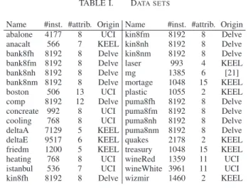
The32 publicly available data sets used in the

experimen-tation are small to medium sized; ranging from approximately 500 to 10000 instances. All but one data set are from the UCI [18], Delve [19] or KEEL [20] repositories. The data sets are described in Table I below, where #inst. is the number of instances and #attrib. is the number of input attributes.

TABLE I. DATA SETS

Name #inst. #attrib. Origin Name #inst. #attrib. Origin abalone 4177 8 UCI kin8fm 8192 8 Delve anacalt 566 7 KEEL kin8nh 8192 8 Delve bank8fh 8192 8 Delve kin8nm 8192 8 Delve bank8fm 8192 8 Delve laser 993 4 KEEL bank8nh 8192 8 Delve mg 1385 6 [21] bank8nm 8192 8 Delve mortage 1048 15 KEEL boston 506 13 UCI plastic 1055 2 KEEL comp 8192 12 Delve puma8fh 8192 8 Delve concreate 992 8 UCI puma8fm 8192 8 Delve cooling 768 8 UCI puma8nh 8192 8 Delve deltaA 7129 5 KEEL puma8nm 8192 8 Delve deltaE 9517 6 KEEL quakes 2178 2 KEEL friedm 1200 5 KEEL treasury 1048 15 KEEL heating 768 8 UCI wineRed 1359 11 UCI istanbul 536 7 UCI wineWhite 3961 11 UCI kin8fh 8192 8 Delve wizmir 1460 2 KEEL

1_{The following names, combining the terms induction, extraction and}

IV. RESULTS.

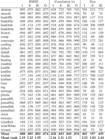
Starting with Experiment 1, using ANN oracles, Table II below shows the results for the three different setups not utilizing oracle data. For comparison, the predictive perfor-mance of the ANNs extracted from are included in the table in the column named O. Looking at the accuracy results, we see that IE is the most successful setup. This is of course a very interesting observation, showing that in scenarios where interpretable models are necessary, more accurate transparent models can be obtained by augmenting the training data with extracted data. Comparing I and E, there are very small dif-ferences in accuracy between inducing and extracting models. When looking at models sizes, however, we see that the extracted models are by far the smallest. This is a clear indication that the general rule extraction paradigm using opaque models is able to reduce the noise typically present in data.

TABLE II. EXPERIMENT1: ACCURACY RESULTS AND SIZE FOR INDUCTION AND EXTRACTION FROMANN

RMSE Correlation (r) Size

I E IE O I E IE O I E IE abalone .095 .079 .082 .077 .628 .725 .705 .742 765 213 772 anacalt .069 .067 .065 .076 .946 .947 .951 .936 50 42 74 bank8fh .106 .094 .094 .090 .816 .854 .854 .867 807 117 521 bank8fm .049 .054 .050 .041 .965 .959 .964 .976 186 116 157 bank8nh .138 .114 .119 .109 .518 .638 .608 .674 1160 306 1095 bank8nm .065 .067 .064 .049 .864 .855 .868 .925 424 319 421 boston .094 .097 .095 .082 .887 .876 .884 .913 134 116 158 comp .037 .042 .038 .038 .980 .974 .979 .978 125 69 100 concreate .082 .101 .085 .088 .916 .866 .908 .900 229 172 281 cooling .056 .073 .059 .073 .976 .958 .974 .959 90 48 113 deltaA .044 .042 .040 .040 .789 .804 .823 .823 774 190 631 deltaE .061 .055 .055 .054 .740 .782 .785 .789 1181 171 884 friedm .098 .095 .094 .051 .857 .861 .865 .962 307 259 313 heating .025 .056 .035 .058 .996 .979 .992 .976 45 41 61 istanbul .104 .081 .088 .082 .565 .704 .656 .707 206 103 311 kin8fh .095 .091 .091 .070 .735 .752 .755 .859 877 497 760 kin8fm .075 .076 .075 .031 .860 .857 .862 .977 531 500 527 kin8nh .157 .144 .144 2.53 1.03 2.44 .609 .737 1271 706 1247 kin8nm .139 .138 .135 .091 .692 .680 .698 .872 973 798 993 laser .052 .057 .051 .037 .956 .949 .958 .977 106 99 116 mg .097 .117 .094 .109 .924 .886 .926 .901 176 109 237 mortage .024 .026 .024 .011 .994 .993 .994 .999 39 40 41 plastic .179 .162 .158 .145 .861 .885 .891 .909 339 129 282 puma8fh .172 .143 .148 .141 .682 .777 .759 .783 1116 92 855 puma8fm .068 .073 .069 .063 .968 .963 .967 .972 178 82 125 puma8nh .156 .138 .137 .137 .755 .803 .805 .806 930 148 728 puma8nm .063 .076 .066 .066 .969 .956 .967 .967 183 132 170 stock .041 .049 .042 .039 .984 .978 .983 .986 82 71 82 treasury .023 .023 .022 .015 .992 .993 .993 .997 35 33 35 wineRed .168 .133 .143 .133 .440 .587 .534 .593 456 224 672 wineWhite .151 .126 .129 .123 .435 .533 .521 .562 1036 309 1227 wizmir .034 .035 .035 .024 .990 .989 .989 .994 60 52 56 Mean .088 .085 .082 .074 .820 .843 .845 .876 465 197 439 Mean rank 2.19 2.22 1.59 - 2.16 2.31 1.53 - 2.53 1.03 2.44

In order to further analyze these results, and to find out if there are any statistically significant differences, we used the recommended procedure in [22] and performed a Friedman test [23], followed by Bergmann-Hommel’s [24] dynamic procedure to establish all pairwise differences. Table III shows

the resulting adjusted p-values. Significant results for α= 0.05

are given in bold. As expected, most of the differences are indeed significant, at this level. Specifically, IE obtained a significantly lower RMSE and a significantly higher correlation

coefficient than both I and E. E, on the other hand, produced significantly smaller models than both I and IE.

TABLE III. EXPERIMENT1: INDUCTION AND EXTRACTION FROM

ANN. ADJUSTED P-VALUES USINGBERGMANN’S PROCEDURE

RMSE r Size

IE vs. E 0.044 0.015 1.9E-08 IE vs. I 0.044 0.015 0.708 E vs. I 0.851 0.708 5.9E-09

Turning to the second part of Experiment 1, i.e., when the opaque models are random forests, Table IV below shows the accuracies and model sizes. First, it should be noted that the random forests are generally more accurate than the ANNs in the previous part, but the differences are often quite small. Nevertheless, the rule extraction clearly benefits from the slightly more accurate random forests. Specifically comparing the evaluated setups, standard rule extraction (E) is actually the most accurate setup on a large number of data sets. When considering all three setups over all data sets, however, IE again obtained the lowest mean rank for both accuracy metrics. Regarding tree sizes, E again produced much smaller models than the other two setups, confirming the reasoning about the ability to filter out anomalies in the training data.

TABLE IV. EXPERIMENT1: ACCURACY RESULTS AND SIZE FOR INDUCTION AND EXTRACTION FROMRF

RMSE Correlation (r) Size

I E IE O I E IE O I E IE abalone .095 .079 .086 .076 .628 .725 .681 .747 765 299 689 anacalt .069 .068 .068 .074 .946 .956 .948 .949 50 25 65 bank8fh .106 .093 .096 .092 .816 .856 .845 .862 807 193 562 bank8fm .049 .053 .050 .043 .965 .960 .964 .976 186 111 151 bank8nh .138 .114 .123 .110 .518 .642 .581 .670 1160 487 1035 bank8nm .065 .064 .063 .051 .864 .867 .871 .926 424 260 368 boston .094 .093 .091 .079 .887 .886 .892 .921 134 87 130 comp .037 .039 .037 .029 .980 .978 .979 .988 125 63 94 concreate .082 .086 .079 .073 .916 .906 .919 .942 229 158 222 cooling .056 .055 .052 .049 .976 .977 .980 .982 90 35 72 deltaA .044 .039 .040 .037 .789 .831 .821 .848 774 211 566 deltaE .061 .054 .055 .053 .740 .792 .778 .800 1181 210 850 friedm .098 .094 .093 .069 .857 .864 .867 .938 307 206 287 heating .025 .035 .026 .026 .996 .991 .995 .996 45 41 46 istanbul .104 .082 .093 .079 .565 .697 .618 .722 206 140 275 kin8fh .095 .090 .091 .075 .735 .756 .752 .848 877 486 732 kin8fm .075 .075 .075 .046 .860 .859 .861 .963 531 404 484 kin8nh .157 .140 .145 .126 .569 .630 .607 .720 1271 677 1124 kin8nm .139 .130 .131 .105 .692 .716 .714 .844 973 615 874 laser .052 .050 .050 .036 .956 .960 .960 .979 106 91 107 mg .097 .097 .092 .089 .924 .923 .930 .936 176 127 170 mortage .024 .026 .025 .012 .994 .993 .994 .999 39 38 39 plastic .179 .174 .165 .161 .861 .872 .880 .896 339 119 312 puma8fh .172 .144 .155 .143 .682 .774 .734 .775 1116 301 866 puma8fm .068 .071 .069 .063 .968 .964 .967 .972 178 89 128 puma8nh .156 .134 .141 .133 .755 .816 .793 .819 930 252 703 puma8nm .063 .069 .065 .059 .969 .964 .968 .976 183 120 156 stock .041 .044 .041 .033 .984 .982 .984 .991 82 64 73 treasury .023 .023 .023 .013 .992 .993 .993 .997 35 31 33 wineRed .168 .136 .151 .128 .440 .570 .497 .628 456 315 557 wineWhite .151 .124 .135 .116 .435 .553 .490 .621 1036 588 1007 wizmir .034 .037 .035 .022 .990 .988 .989 .996 60 47 55 Mean .088 .082 .083 .072 .820 .851 .839 .882 465 215 401 Mean rank 2.47 1.88 1.66 - 2.41 1.91 1.69 - 2.84 1.00 2.16

Table V below shows adjusted p-values from Bergmann’s

bold. Comparing these results (obtained using random forests) to the results produced using ANNs, the most important difference is that using standard rule extraction (E) is now a very strong choice. E is actually significantly more accurate than standard induction (I), and the resulting models are most often as accurate as the ones produced using IE. This is despite the fact that the regression trees built by E are significantly smaller than the other two setups.

TABLE V. EXPERIMENT1: INDUCTION AND EXTRACTION FROMRF. ADJUSTED P-VALUES USINGBERGMANN’S PROCEDURE

RMSE r Size

IE vs. E 0.574 0.382 3.7E-06 IE vs. I 0.015 0.012 0.006 E vs. I 0.024 0.046 4.9E-13

Summarizing Experiment 1, the most important finding is that the use of a highly accurate opaque model as a pre-processing step is clearly beneficial for generating transparent regression models. The most accurate setup overall combined original training data, with training data labeled by the opaque model, in the generation phase. In addition, utilizing data la-beled by the opaque model also produced significantly smaller regression trees.

Turning to Experiment 2, i.e., when the oracle data are included, Table VIII, placed after the references section, shows accuracy results and tree sizes using ANNs as oracles. The most obvious result is the benefit from utilizing oracle data. More specifically, setups combining oracle data with training data (IX and IEX) are the most accurate. Interestingly enough, these setups are more accurate than X, i.e., using only the oracle data. X is actually even slightly less accurate than EX, which combines extracted data with oracle data. Still, the three setups not using oracle data (I, E, IE) have the worst accuracy, so the oracle coaching procedure paid off. Looking at tree sizes, X produced the most compact trees for all data sets. With this in mind, if the purpose is to explain or analyse the predictions for a specific production set, setup X is a viable choice. Another important observation is that setups using extracted data (E, EX) produce much smaller models than setups generated on training data. This confirms the findings in Experiment 1 that highly accurate opaque models can serve as pre-processing tools when building transparent predictive models. Finally, it should be noted that the increased accuracy of IEX and IX do not result in more complex trees, compared to I.

Table VI below, which shows adjusted p-values from Bergmann’s procedure, confirms most of the observed differ-ences to be statistically significant. Specifically, both setups combining training and oracle data (IX and IEX) are signifi-cantly more accurate than all three setups not utilizing oracle data (I, E, IE). Regarding model sizes, the setups using only oracle data (E, EX and X) all produced significantly smaller trees than setups including original training data, i.e., I, IX and IEX.

TABLE VI. EXPERIMENT2: ANNS AS ORACLES. ADJUSTED P-VALUES USINGBERGMANN’S PROCEDURE

RMSE r Size

IX vs. E 7.4E-06 9.6E-07 1.9E-10 IEX vs. E 9.7E-06 2.5E-06 1.9E-07 IX vs. I 6.3E-05 4.8E-05 1.346 IEX vs. I 7.3E-05 9.6E-05 1.930 EX vs. E 0.003 0.003 1.154 IX vs. IE 0.018 0.015 1.346 EX vs. I 0.018 0.035 2.6E-05 X vs. E 0.018 0.010 0.195 IEX vs. IE 0.018 0.020 1.930 X vs. I 0.051 0.084 3.1E-15 IX vs. X 0.442 0.216 6.3E-18 IE vs. E 0.442 0.216 1.8E-08 IEX vs. X 0.442 0.216 9.8E-14 EX vs. IE 0.467 0.869 2.6E-05 EX vs. IX 0.700 0.320 8.1E-07 IE vs. I 0.700 0.444 1.930 IEX vs. EX 0.700 0.320 1.5E-04 X vs. IE 0.707 0.934 3.7E-15 E vs. I 1.868 1.254 1.8E-08 EX vs. X 1.868 1.457 0.003 IEX vs. IX 1.868 1.457 1.346

The results for Experiment 2 when using the random forest as the oracle, are presented in Table IX, at the end of the paper. Again, we see that setups using oracle data are the most accurate. The most interesting observation is perhaps that EX here performs relatively better than when using ANNs. The reason is, of course, the slightly stronger oracle. Actually, in this setting, EX is almost as accurate as IX, despite the fact that the trees are (on average) less than half the size.

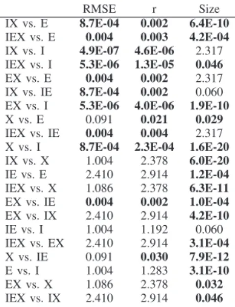
As seen in Table VII below, there are a large number of

statistically significant differences for α= 0.05. Specifically,

all three setups combining training and/or extraction data with oracle data (IX, EX, IEX) are significantly more accurate than all setups not utilizing oracle data, i.e., I, E and IE.

TABLE VII. EXPERIMENT2: RFS AS ORACLES. ADJUSTED P-VALUES USINGBERGMANN’S PROCEDURE

RMSE r Size

IX vs. E 8.7E-04 0.002 6.4E-10 IEX vs. E 0.004 0.003 4.2E-04 IX vs. I 4.9E-07 4.6E-06 2.317 IEX vs. I 5.3E-06 1.3E-05 0.046 EX vs. E 0.004 0.002 2.317 IX vs. IE 8.7E-04 0.002 0.060 EX vs. I 5.3E-06 4.0E-06 1.9E-10 X vs. E 0.091 0.021 0.029 IEX vs. IE 0.004 0.004 2.317 X vs. I 8.7E-04 2.3E-04 1.6E-20 IX vs. X 1.004 2.378 6.0E-20 IE vs. E 2.410 2.914 1.2E-04 IEX vs. X 1.086 2.378 6.3E-11 EX vs. IE 0.004 0.002 1.0E-04 EX vs. IX 2.410 2.914 4.2E-10 IE vs. I 1.004 1.192 0.060 IEX vs. EX 2.410 2.914 3.1E-04 X vs. IE 0.091 0.030 7.9E-12 E vs. I 1.004 1.283 3.1E-10 EX vs. X 1.086 2.378 0.032 IEX vs. IX 2.410 2.914 0.046

Based on the correlation coefficient r, X is also signifi-cantly more accurate than the three setups not using oracle

data. Using RMSE, however, the superior accuracy is only significant against I. Looking at model sizes, the picture is almost identical to when ANNs are used as oracles, i.e., all setups using extracted data (but not training data) produced significantly smaller trees than setups using training data.

From these results, it is obvious that the oracle coaching paradigm works as intended in the regression context. Specifi-cally, setups including oracle data are most often significantly more accurate than setups using only training or extraction data. Furthermore, generating models on the smoothed ver-sion of the training data (the extraction data), will lead to significantly more compact models, compared to using original training data. Interestingly enough, this study indicates that the quality of the oracle is not vital, as long as it is accurate enough. Specifically, the fairly large differences in accuracy between the ANNs and the random forests, did not carry over to the coached regression trees.

V. CONCLUDING REMARKS.

We have in this paper introduced oracle coaching for predictive regression. The purpose of this method is to produce interpretable models, and it applies to the very common situation where the predictive model is built for a specific production set with known input vectors. In oracle coaching, a highly accurate, but opaque, model (“the oracle”) is first induced from standard training data. The oracle is then used to label both training instances and production instances. In the last step, interpretable models are trained using different combinations of these data sets. The method is very general, since any opaque model can serve as the oracle and any technique producing transparent models can benefit from this procedure. The experimental results show that for predictive regression, the use of oracle coaching produced significantly more accurate regression trees, compared to using standard induction. In addition, the results also show that even in situations where the production set inputs are not available, using an oracle as a pre-processing step, just to reduce the noise in the training data, produced significantly more accurate and/or smaller regression trees.

REFERENCES

[1] P. Domingos, “Knowledge discovery via multiple mod-els,” Intelligent Data Analysis, vol. 2, pp. 187–202, 1998. [2] R. Blanco-Vega, J. Hernández-Orallo, and M. Ramírez-Quintana, “Analysing the trade-off between comprehen-sibility and accuracy in mimetic models,” in Discovery Science, ser. LNCS. Springer, 2004, vol. 3245, pp. 338– 346.

[3] R. Andrews, J. Diederich, and A. B. Tickle, “Survey and critique of techniques for extracting rules from trained artificial neural networks,” Knowl.-Based Syst., vol. 8, no. 6, pp. 373–389, 1995.

[4] M. W. Craven and J. W. Shavlik, “Extracting tree-structured representations of trained networks,” in Ad-vances in Neural Information Processing Systems. MIT Press, 1996, pp. 24–30.

[5] A. A. Freitas, “A survey of evolutionary algorithms for data mining and knowledge discovery,” in Advances in

Evolutionary Computation. Springer-Verlag, 2002.

[6] A. Dobra and J. Gehrke, “Secret: A scalable linear

regression tree algorithm,” in KDD. New York, NY,

USA: ACM, 2002, pp. 481–487.

[7] L. Breiman, J. Friedman, C. J. Stone, and R. A.

Ol-shen, Classification and Regression Trees. Chapman &

Hall/CRC, 1984.

[8] J. Fürnkranz, D. Gamberger, and N. Lavraˇc, Foundations of Rule Learning. Springer Publishing Company, 2012. [9] L. Breiman, “Bagging predictors,” Machine Learning,

vol. 24, no. 2, pp. 123–140, 1996.

[10] M. Craven and J. Shavlik, “Rule extraction: Where do we go from here?” University of Wisconsin Machine Learning Research Group working Paper 99-1, 1999. [11] Z.-H. Zhou, “Rule extraction: using neural networks or

for neural networks?” J. Comput. Sci. Technol., vol. 19, no. 2, pp. 249–253, 2004.

[12] U. Johansson, T. Löfström, R. König, and L. Niklasson, “Why not use an oracle when you got one?” Neural Information Processing: Letters and Reviews, vol. 10, no. 8-9, pp. 227–236, 2006.

[13] U. Johansson and L. Niklasson, “Evolving decision trees

using oracle guides,” in CIDM. IEEE, 2009, pp. 238–

244.

[14] U. Johansson, C. Sönströd, and T. Löfström, “Oracle coached decision trees and lists,” in IDA, ser. LNCS, vol.

6065. Springer, 2010, pp. 67–78.

[15] C. Sönströd, U. Johansson, H. Boström, and U. Norinder,

“Pin-pointing concept descriptions.” in SMC. IEEE,

2010, pp. 2956–2963.

[16] U. Johansson, C. Sönströd, T. Löfström, and H. Boström, “Obtaining accurate and comprehensible classifiers using oracle coaching,” Intell. Data Anal., vol. 16, no. 2, pp. 247–263, 2012.

[17] L. Breiman, “Random forests,” Machine Learning, vol. 45, no. 1, pp. 5–32, 2001.

[18] K. Bache and M. Lichman, “UCI machine learning repository,” 2013. [Online]. Available: http://archive.ics. uci.edu/ml

[19] C. E. Rasmussen, R. M. Neal, G. Hinton, D. van Camp, M. Revow, Z. Ghahramani, R. Kustra, and R. Tibshirani, “Delve data for evaluating learning in valid experiments,” www. cs. toronto. edu/delve, 1996.

[20] J. Alcalá-Fdez, A. Fernández, J. Luengo, J. Derrac, and S. García, “Keel data-mining software tool: Data set repository, integration of algorithms and experimental analysis framework,” Multiple-Valued Logic and Soft Computing, vol. 17, no. 2-3, pp. 255–287, 2011. [21] G. W. Flake and S. Lawrence, “Efficient svm regression

training with smo,” Machine Learning, vol. 46, no. 1-3, pp. 271–290, 2002.

[22] S. García and F. Herrera, “An extension on statistical comparisons of classifiers over multiple data sets for all pairwise comparisons,” Journal of Machine Learning Research, vol. 9, no. 2677-2694, p. 66, 2008.

[23] M. Friedman, “The use of ranks to avoid the assumption of normality implicit in the analysis of variance,” Journal of American Statistical Association, vol. 32, pp. 675–701, 1937.

[24] B. Bergmann and G. Hommel, “Improvements of gen-eral multiple test procedures for redundant systems of

hypotheses,” in Multiple Hypotheses Testing. Springer,

T ABLE VIII. E X P E R IM E N T 2 : A C C U R A C Y R E S U L T S A N D S IZ E S U S IN G A N N S A S O R A C L E S RMSE Correlation (r) Size I E IE X IX EX IEX I E IE X IX EX IEX I E IE X IX EX IEX abalone .095 .079 .082 .078 .082 .079 .079 .628 .725 .705 .732 .706 .728 .728 765 213 772 120 788 216 763 anacalt .069 .067 .065 .095 .068 .070 .066 .946 .947 .951 .900 .945 .942 .947 50 42 74 17 54 43 76 bank8fh .106 .094 .094 .092 .096 .093 .092 .816 .854 .854 .859 .847 .857 .859 807 117 521 96 779 117 500 bank8fm .049 .054 .050 .049 .047 .052 .049 .965 .959 .964 .966 .968 .962 .966 186 116 157 97 179 116 156 bank8nh .138 .114 .119 .111 .118 .112 .113 .518 .638 .608 .661 .623 .655 .649 1160 306 1095 170 1175 309 1080 bank8nm .065 .067 .064 .056 .054 .058 .057 .864 .855 .868 .900 .909 .891 .897 424 319 421 158 433 324 421 boston .094 .097 .095 .089 .074 .079 .077 .887 .876 .884 .894 .928 .917 .923 134 116 158 19 138 121 160 comp .037 .042 .038 .040 .036 .041 .038 .980 .974 .979 .976 .981 .975 .979 125 69 100 58 118 69 99 concreate .082 .101 .085 .101 .075 .093 .082 .916 .866 .908 .863 .929 .888 .914 229 172 281 38 244 175 282 cooling .056 .073 .059 .078 .055 .073 .060 .976 .958 .974 .953 .977 .959 .972 90 48 113 24 96 48 111 deltaA .044 .042 .040 .041 .040 .041 .039 .789 .804 .823 .813 .824 .811 .830 774 190 631 130 777 192 615 deltaE .061 .055 .055 .054 .056 .055 .054 .740 .782 .785 .785 .776 .785 .791 1181 171 884 141 1162 172 855 friedm .098 .095 .094 .071 .065 .067 .070 .857 .861 .865 .922 .938 .933 .925 307 259 313 46 319 269 319 heating .025 .056 .035 .065 .027 .055 .038 .996 .979 .992 .971 .995 .979 .990 45 41 61 25 49 41 61 istanb ul .104 .081 .088 .082 .085 .080 .081 .565 .704 .656 .699 .686 .716 .706 206 103 311 19 229 107 317 kin8fh .095 .091 .091 .077 .082 .082 .084 .735 .752 .755 .830 .803 .801 .791 877 497 760 245 865 503 753 kin8fm .075 .076 .075 .048 .058 .060 .064 .860 .857 .862 .945 .918 .912 .899 531 500 527 246 540 507 530 kin8nh .157 .144 .144 .127 .133 .132 .133 .569 .604 .609 .709 .681 .676 .675 1271 706 1247 284 1293 718 1242 kin8nm .139 .138 .135 .103 .106 .113 .115 .692 .680 .698 .833 .821 .795 .784 973 798 993 293 1004 814 1004 laser .052 .057 .051 .057 .040 .046 .044 .956 .949 .958 .949 .975 .966 .970 106 99 116 35 111 101 117 mg .097 .117 .094 .114 .091 .113 .099 .924 .886 .926 .892 .932 .894 .919 176 109 237 49 185 111 241 mortage .024 .026 .024 .025 .021 .021 .021 .994 .993 .994 .993 .996 .995 .995 39 40 41 25 39 40 41 plastic .179 .162 .158 .174 .157 .157 .152 .861 .885 .891 .865 .893 .892 .899 339 129 282 34 338 131 269 puma8fh .172 .143 .148 .142 .154 .142 .145 .682 .777 .759 .780 .741 .778 .771 1116 92 855 83 1112 92 830 puma8fm .068 .073 .069 .070 .067 .072 .068 .968 .963 .967 .965 .968 .964 .967 178 82 125 75 168 83 123 puma8nh .156 .138 .137 .138 .142 .137 .136 .755 .803 .805 .803 .794 .804 .810 930 148 728 124 927 148 710 puma8nm .063 .076 .066 .073 .062 .074 .066 .969 .956 .967 .959 .971 .958 .967 183 132 170 114 183 133 169 stock .041 .049 .042 .046 .036 .042 .038 .984 .978 .983 .980 .988 .983 .987 82 71 82 35 83 72 81 treasury .023 .023 .022 .028 .019 .020 .020 .992 .993 .993 .988 .995 .994 .994 35 33 35 22 35 33 35 wineRed .168 .133 .143 .133 .140 .132 .134 .440 .587 .534 .593 .553 .598 .591 456 224 672 53 492 230 686 wineWhite .151 .126 .129 .124 .128 .125 .124 .435 .533 .521 .554 .528 .545 .556 1036 309 1227 132 1075 313 1228 wizmir .034 .035 .035 .030 .032 .033 .034 .990 .989 .989 .992 .991 .990 .990 60 52 56 39 59 52 55 Mean .088 .085 .082 .082 .076 .080 .077 .820 .843 .845 .860 .862 .861 .864 465 197 439 95 470 200 435 Mean rank 5.25 5.50 4.44 3.75 2.66 3.56 2.84 5.19 5.59 4.38 3.81 2.63 3.69 2.72 5.44 2.19 5.41 1.00 5.84 2.94 5.19

T ABLE IX. E X P E R IM E N T 2 : A C C U R A C Y R E S U L T S A N D S IZ E S U S IN G R F S A S O R A C L E S RMSE Correlation (r) Size I E IE X IX EX IEX I E IE X IX EX IEX I E IE X IX EX IEX abalone .095 .079 .086 .077 .083 .078 .081 .628 .725 .681 .741 .703 .735 .715 765 299 689 108 775 292 683 anacalt .069 .068 .068 .093 .066 .068 .067 .946 .956 .948 .912 .950 .956 .952 50 25 65 10 53 25 66 bank8fh .106 .093 .096 .093 .097 .093 .094 .816 .856 .845 .856 .842 .857 .852 807 193 562 91 779 184 544 bank8fm .049 .053 .050 .051 .048 .052 .049 .965 .960 .964 .965 .968 .962 .965 186 111 151 84 177 110 149 bank8nh .138 .114 .123 .111 .119 .112 .116 .518 .642 .581 .660 .612 .655 .627 1160 487 1035 161 1168 469 1027 bank8nm .065 .064 .063 .057 .057 .059 .059 .864 .867 .871 .901 .898 .890 .889 424 260 368 125 423 260 365 boston .094 .093 .091 .089 .074 .083 .079 .887 .886 .892 .895 .930 .912 .920 134 87 130 18 135 90 130 comp .037 .039 .037 .036 .036 .037 .037 .980 .978 .979 .981 .981 .979 .980 125 63 94 48 118 62 91 concreate .082 .086 .079 .089 .069 .078 .073 .916 .906 .919 .903 .940 .927 .934 229 158 222 37 235 157 224 cooling .056 .055 .052 .060 .052 .054 .051 .976 .977 .980 .972 .979 .978 .980 90 35 72 22 87 35 69 deltaA .044 .039 .040 .038 .040 .039 .039 .789 .831 .821 .838 .827 .835 .832 774 211 566 112 749 207 552 deltaE .061 .054 .055 .054 .056 .054 .054 .740 .792 .778 .794 .774 .793 .786 1181 210 850 117 1140 200 823 friedm .098 .094 .093 .082 .075 .080 .080 .857 .864 .867 .904 .915 .906 .904 307 206 287 44 315 209 291 heating .025 .035 .026 .046 .024 .034 .026 .996 .991 .995 .985 .996 .992 .995 45 41 46 24 45 41 46 istanb ul .104 .082 .093 .080 .085 .079 .082 .565 .697 .618 .709 .676 .714 .694 206 140 275 19 228 143 278 kin8fh .095 .090 .091 .080 .085 .085 .086 .735 .756 .752 .820 .788 .789 .781 877 486 732 229 867 480 725 kin8fm .075 .075 .075 .057 .064 .067 .069 .860 .859 .861 .930 .899 .892 .885 531 404 484 224 531 405 481 kin8nh .157 .140 .145 .130 .138 .134 .137 .569 .630 .607 .694 .650 .669 .652 1271 677 1124 224 1286 667 1125 kin8nm .139 .130 .131 .113 .117 .119 .120 .692 .716 .714 .806 .778 .771 .763 973 615 874 233 981 610 876 laser .052 .050 .050 .052 .042 .043 .043 .956 .960 .960 .957 .972 .971 .971 106 91 107 33 108 93 109 mg .097 .097 .092 .097 .081 .088 .084 .924 .923 .930 .923 .946 .936 .942 176 127 170 49 179 128 171 mortage .024 .026 .025 .025 .021 .022 .022 .994 .993 .994 .993 .995 .995 .995 39 38 39 24 39 39 39 plastic .179 .174 .165 .186 .163 .171 .161 .861 .872 .880 .852 .883 .878 .888 339 119 312 34 350 121 305 puma8fh .172 .144 .155 .143 .156 .143 .150 .682 .774 .734 .777 .733 .776 .751 1116 301 866 86 1110 279 847 puma8fm .068 .071 .069 .071 .067 .071 .068 .968 .964 .967 .965 .968 .965 .967 178 89 128 69 167 87 126 puma8nh .156 .134 .141 .135 .142 .134 .138 .755 .816 .793 .814 .791 .817 .803 930 252 703 112 918 238 690 puma8nm .063 .069 .065 .069 .062 .068 .064 .969 .964 .968 .965 .971 .965 .969 183 120 156 100 180 120 155 stock .041 .044 .041 .042 .036 .038 .037 .984 .982 .984 .984 .988 .986 .987 82 64 73 32 81 64 73 treasury .023 .023 .023 .027 .020 .020 .021 .992 .993 .993 .989 .994 .994 .994 35 31 33 22 35 31 33 wineRed .168 .136 .151 .129 .139 .130 .135 .440 .570 .497 .618 .557 .616 .576 456 315 557 50 487 322 565 wineWhite .151 .124 .135 .118 .126 .120 .124 .435 .553 .490 .610 .547 .589 .557 1036 588 1007 138 1063 585 1015 wizmir .034 .037 .035 .030 .032 .034 .034 .990 .988 .989 .992 .991 .989 .990 60 47 55 37 59 48 54 Mean .088 .082 .083 .080 .077 .078 .078 .820 .851 .839 .866 .858 .865 .859 465 215 401 85 465 213 398 Mean rank 5.78 4.97 4.81 3.59 2.72 3.09 3.03 5.75 5.00 4.91 3.53 2.88 2.84 3.09 6.19 2.59 4.88 1.00 6.09 2.53 4.72