The Impact of Short Selling on Stock Returns – An Event
Study in Sweden
Thomas Kouzoubasis & Homam Al Sakka
June 3, 2021
Bachelor Thesis within Finance
Division of Business and Social Science Mälardalen University
SE-721 23 Västerås, SWEDEN Supervisor: Christos Papahristodoulou
Bachelor Thesis within Finance
Title: The Impact of Short Selling on Stock Returns – An Event Study in Sweden Authors: Thomas Kouzoubasis* and Homam Al Sakka†
Tutor: Christos Papahristodoulou Date: June 3, 2021
Keywords: Short selling, Stock returns, Regulations, Sweden, Informed short selling, Un-informed short selling, Regression analysis
Abstract
Short selling, and its informational role in the formation of stock prices have been the epicenter of prior literature. Is there a relationship between short selling and abnormal returns? While numerous studies found a negative relationship, researchers do not unanimously agree on the existence, nor the strength, of this relationship. Using net short positions extracted from the registry of the FI for stocks listed in the OMX Stockholm 30 Exchange from January 2017 to December 2020, we examine this relationship exclusively in Sweden. The results have been scrutinized via regression analysis to verify if there is any significant relationship between the announcements of total net short positions and the non-adjusted, as well as the risk-adjusted abnormal returns.
We did not find enough evidence to validate previous studies that supported the notion that heavily shorted stocks generate negative abnormal returns for the long buyers. There was a perceptible increase in both risk-adjusted and non-adjusted abnormal returns within a three-day window after the announcement of a short position. Yet, the value was merely zero, infer-ring that a higher level of short interest does not lead to negative stock returns.
Acknowledgements
We would like to thank our supervisor Christos Papahristodoulou for his feedback and sugges-tions during our time of writing this thesis. The help was valuable to evaluate and improve the quality of our work.
thomaskouzou@gmail.com † haa18001@student.mdh.se
Contents
1 Introduction ... 1
1.1 Background ... 1
1.1.1 Short Selling Regulations – A Brief History and Comparison ... 2
1.1.2 Short Selling & Market Efficiency ... 4
1.2 Purpose ... 7
1.3 Research Aim ... 8
2 Literature Review & Hypothesis ... 9
2.1 Informed Short Selling ... 9
2.2 Uninformed Short Selling ... 10
2.3 Summary & Hypothesis ... 12
3 Methodology & Data... 14
3.1 Event Intervals for Abnormal returns... 14
3.2 Variables... 15
3.2.1 Abnormal Returns ... 15
3.2.2 Independent Variable: Net Short Position ... 18
3.2.3 Dummy (Binary) Variable: Multiple Announcements ... 18
3.3 The Model ... 19
3.4 Data ... 21
3.4.1 Data Collection ... 21
3.4.2 Data Adjustments & Sample ... 21
4 Estimates & Analysis ... 23
4.1 Descriptive Statistics ... 23
4.2 Regression Estimates... 24
4.2.1 Periods (0,t) ... 25
4.2.2 Periods (-t,t) ... 27
5 Conclusion ... 28
6 Limitations & Recommendations for Future Research ... 29
List of References ... 31
Appendices ... 36
Appendix A: Short Selling Regulations ... 36
Table A.1 Restrictions on Short Selling in 2008 & 2020 ... 36
Appendix B: Dataset ... 37
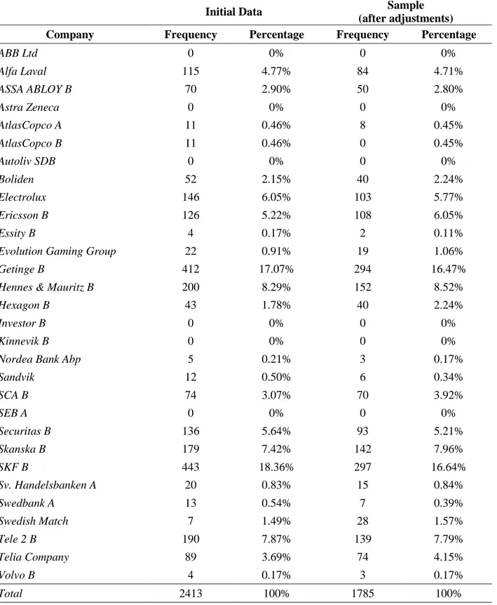
Table B.1 Overview of the firms that were shorted ... 37
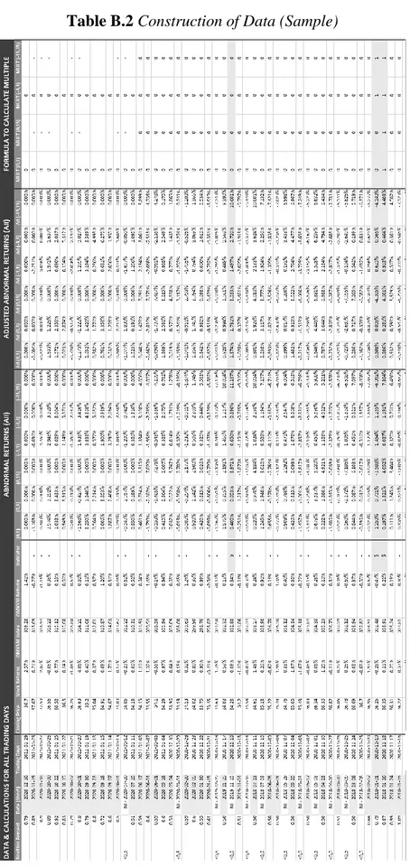
Table B.2 Construction of Data (Sample) ... 38
Table C.1 Regression results for Periods (0,1), (0,3), and (0,15) ... 39 Table C.2 Regression results for Periods (-1,1), (-3,3), and (-15,15) ... 39 Table C.3 Regression results for Periods (-3,1), (-5,2), and (-8,3) ... 40
1
1 Introduction
1.1 Background
Investors can play the market in multiple ways to make money. The most conventional investing technique while trading is to go long on a stock or bond, where an investor holds an asset with the expectation that the security will go up in value. More advanced investors can utilize alternative strategies such as options contract to reduce risks or to increase cost-efficiency. Along with that, investors can also earn a profit on securities where their price drops. One example is put-options which is a contract that the buyer pays a premium to have the right, but he is not obliged, to sell a specific number of shares at an agreed-upon strike price. A riskier technique that follows the same pattern is short selling.
More explicitly, short selling also called “going short” or “shorting” implies selling se-curities that the investor has borrowed. Later they need to return what they owe to the lender. Short sellers have a bearish expectation of the market; thus, when investors buy the shares back at a lower price to return them to the lenders, they have made a profit because they had initially sold them at a higher price. When the short seller is unable to return the borrowed shares, i.e., due to bankruptcy, the responsibility falls to the broker. Though, there is an amount that is required to be deposited into a margin account, also known as margin requirements. That way, the broker eliminates risks that are associated with lending. Lenders, on the other hand, can receive more income over time under fee agreements with their broker, so they benefit from a passive income (Reed, 2013; Fabozzi, 2004). Swedish brokers such as Avanza, follow a standardized framework of agreements where the obligations between the lender and the broker are similar (Avanza, n.d.). Some of the costs of short selling are margin interest e.g., expenses can be too high especially when a short position is open over an extended period, stock borrowing costs, and finally dividends and other payments.
Short sellers constitute approximately more than 20% of trading volume on average in most markets and are generally considered as traders with access to value-relevant in-formation (Boehmer, Jones, & Zhang, 2008). Short selling seems to be a controversial topic. The “scandal” in early January 2021 with the GME stock unprecedented price increase that was derived from retail investors to fight off hedge funds only brought new
2
subjects for thought1. The practice of short selling becomes more apparent when the market faces disruptions. 2020 has been a rough year, COVID-19 has created a lot of uncertainty and that has also been depicted on the stock market. It was a similar reaction to the financial crisis in 2008. The stock market was plumbing, and short interests started rising, as a result, short sale bans were introduced around the world. The strategy of short selling has raised moral discussions concerning market manipulation, but also its utility to speculate on economic downturns (Allen & Gale, 1992; Durston, 2021). Market efficiency, short selling bans, liquidity, and information asymmetry has also been the focal point of prior research. In general, there have been a lot of studies on short selling, however, not many studies encompass Nordic countries. The paper continues with the background by exploring some of the studies regarding the prohibition of short selling and market efficiency.
1.1.1 Short Selling Regulations – A Brief History and Comparison
Short selling restrictions first appeared in 1610 in the Amsterdam stock exchange (Bris, Goetzmann, & Zhu, 2007). As mentioned earlier, various scholars have debated over the practice of short selling. Thus, many started arguing the applicability of short selling on the stock market, whether it can induce liquidity and efficiency. This is regarding the fact that short selling can provide price and value adjustment on shares that are over-priced by considering the private negative signals short sellers have on a share. Many believed that short sellers are the cause for stock market declines (Bris et al., (2007). Hence, policymakers, imposed temporally bans to achieve market stabilization by con-trolling the volume of short selling during a bearish or volatile market. For example, the Securities and Exchange Commission (SEC) implemented a trading regulation between 1938 and 2007 i.e., the short-sale rule that restricted the short selling of a stock that its price was declining. This rule was lifted in 2007 and in 2010 SEC implemented a new order which prohibits short selling when a share has dropped 10% or more (SEC, 2021). Other countries such as Japan, banned naked short selling2 in October 2008. They ex-tended the ban several times, and then the ban became permanent five years later in 2013 (Osaki, 2013).
1 To read more about the GME topic, see here: Usman W. Chohan (2021), “Counter-Hegemonic Fi-nance: The Gamestop Short Squeeze”, https://papers.ssrn.com/sol3/papers.cfm?abstract_id=3775127. 2 Naked shorting is the illegal practice of short selling shares. In other words, when traders short shares that never existed, thus shares that they never borrowed. Despite being illegal, naked shorting continues to happen due to loopholes between paper and electronic trading systems.
3
The European Securities and Markets Authority (ESMA) allows countries to carry out short selling restrictions in two ways, short-term ban, and long-term ban. In the case where a country plans to impose a long-term ban, ESMA will assess the situation and will declare whether the measures and their duration are appropriate to tackle the threat (ESMA, n.d.). Another type of regulation that is worth mention is that of Credit Default Swaps (CDS). Lender faces a risk whenever they lend to another investor, the risk is that the borrower may default the repayment. This risk is known as the credit risk. The pur-pose of CDS is to provide protection over the credit risk (Saunders, 2010). Before the 2008 crisis protection buyers were free to buy put options and they had the same right to be compensated when their non-owned asset crashed. Past literature argues that CDS played a big part in contributing to the global financial crisis in 2008 (Senarath & Copp, 2015).
The consensus among researchers is that banning short selling not only has no benefits, but also harms market efficiency and lessens liquidity in the stock market. Chang et al. (2014) examined the impact of short selling and margin-trading and proved that traders try to adjust overpriced shares by taking short positions, thus encouraging market effi-ciency. When short selling restrictions were lifted in 2010 in China, an increase in price efficiency and a decrease in market volatility were detected (Chang, Luo, & Ren, 2014). In addition, another study found similar results. Specifically, Bernal et al., (2014) claim that prohibition of covered short selling raises bid-ask spread and reduces the trading volume. Moreover, two researchers studied 12,600 stocks in 26 countries and supported the notion that stocks with stronger short sale constraints have lower price efficiency (Saffi & Sigurdsson, 2010). In general, it comes to an agreement that restrictions on short selling degrade market efficiency, and the only regulation that showed a less neg-ative impact on trading volume and market efficiency was on naked short selling (Bernal, Herinckx, & Szafarz, 2014). On top of that, a study that was targeting the main European countries during COVID-19 also verifies the prior belief. Higher information asymmetry, lower liquidity, and lower abnormal returns were shown on stocks that were banned (Siciliano & Ventoruzzo, 2020).
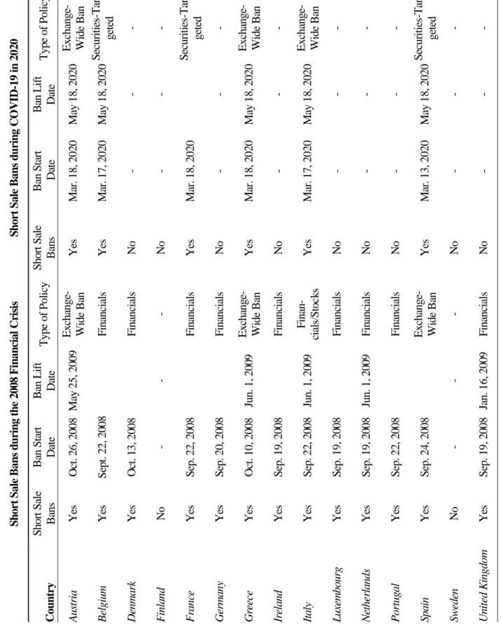
Under both recessions in 2008 and 2020, Sweden decided not to prohibit short selling. Two bachelor’s theses that were conducted in Sweden, concluded that short sale con-straints will not benefit the Swedish market (Lalehzar & Lennartsson, 2015; Andersson,
4
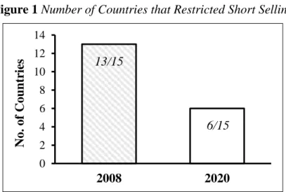
Bodestedt, & Hjortsjö, 2009). However, these studies are relatively old, therefore, ex-tended research on more recent short selling activity can be useful. Additionally, we compiled a small sample that consisted of some of the major European countries from two previous studies, as seen in Figure 1 (Siciliano & Ventoruzzo, 2020; Beber & Pagano, 2013). It appears that there was a 54% decrease in the number of countries that prohibited short selling in 2008 compared to 20203. This suggests that more European countries decide to not take strict measures on short selling during stretches of volatile equity markets.
Figure 1 Number of Countries that Restricted Short Selling
1.1.2 Short Selling & Market Efficiency
The term market efficiency or commonly known as the efficient market hypothesis (EMH), comes from a paper written by Eugene F. Fama in 1970. Precisely, Fama sum-marized: The stock market is “efficient” in the sense that stock prices adjust very rapidly
to new information. In other words, to what degree available information affects the
fluctuation of a stock. If the market is efficient then nobody would be able to “beat” the market because no security is overvalued or undervalued4. Here, it is important to men-tion that the term is theoretical because no one has a clear definimen-tion of how to perfectly measure “market efficiency” (Fama, 1970). According to Fama (1965; 1995), a stock market where price changes in individual securities have the same distribution and are independent of each other is by their definition a random walk market. That brings us to
3 See Appendix A, Table A.1 for more details.
4 Though, nowadays computers can operate under smart algorithms where the reaction can happen at a tenth of a second when a piece of new information is instantaneously revealed and beat those who could not react sufficiently quick or tried to enter their position manually.
0 2 4 6 8 10 12 14 2008 2020 No. of Coun tr ies 13/15 6/15
5
another noteworthy concept that explains how available information affects the move-ment of a stock.
The random walk hypothesis came from Kendal (1953) where he supports that when stock prices follow a random walk, it means that the stock price changes at random and this cannot be predicted. This assumption is valid as long as investors cannot use the information of past actions of changes in stock prices to increase profits (Kendal, 1953). In other words, the share price can only increase or decrease when newly available in-formation enters the market. Prices will always adjust when investors try to take ad-vantage of past activity, thus a stock price will always represent its fundamental value. However, this theory has been debated, and until now, no consensus has been reached. It is being argued that professional analysts can somewhat predict the direction of a stock through technical historical analysis (Malkiel, 2020). In chapter 2, we explain further, why short sellers have different reasons to believe that a stock price is inflated.
1.1.2.1 Positive Contribution of Short Selling
Short selling can be very healthy for a financial market situation where it enhances the liquidity within the market situation. Liquidity within the financial markets situation is the ability of traders to be able to make sales and purchases of stocks at the same time (Hatcher, 2020). When traders short stock in the market, they avail different stocks within the market for the buyers to partake of and they are also able to sell. This enhances the efficiency of the different trading activities within the financial market situation, which is very helpful for continued business operations within the financial markets. Short selling can also enhance the price stability of the different stocks within the market environment (Hatcher, 2020). Price stability is mainly influenced by the demand of the different stocks within the market environment. When traders are able to short stock from time to time, they are able to supply stocks into the markets. Later, when they buy these stocks back after the speculation periods, they create the necessary demand that is required to stabilize the prices of the different stocks within the financial environments. Therefore, it is worthwhile noting that short selling can play crucial roles in enhancing market efficiency as well as stabilizing the different prices of the stocks by manipulating the factors of demand and supply (Li, Lin, Zhang, & Chen, 2018). However, there is a downside to the practice of short selling with relevance to the time period under which
6
the practice is undertaken, the frequency, and the number of stocks that are sold short at a given time. When a limited number of traders are involved in short selling over a short-defined period of time, the practice becomes practical and favorable for the health of the market in terms of its efficiency and price stabilization (Hatcher, 2020).
1.1.2.2 Negative Contribution of Short Selling
Short selling can also have adverse negative effects on the markets depending on the scale on which it is practiced and the likelihood of the market (Boulton & Braga-Alves, 2020). When many people are involved in selling stocks short, a huge part of the market is speculated. In the sense that if all these people lose by having the stock rise in prices rather than fall, they will have to buy them back more expensively than they sold, mean-ing that they are likely to make losses in the short run. If a huge number of traders within the financial markets make losses, it could be dangerous for the market as a whole. This case has been observed in some established economies of the world that brought them down to their knees. The widespread negative effect is not only felt within the market but also within the different individual industries and markets where different companies that are affected operate and undertake their activities.
In some other instances, the extensive short selling practiced by traders could result in widespread fear among all the traders that are involved within the market situation (Boulton & Braga-Alves, 2020). This fear can fuel improper investment decisions as people are trying to secure their investments from negative market impacts such as mar-ket recessions and depressions that could make them lose everything. This results in panic selling that they will end up regretting in the long run. Uncontrolled short selling within the financial and securities markets can have adverse effects on the overall busi-ness environments because they are the avenues that busibusi-nesses use to raise funds and sustain the economies around their industries (Boulton & Braga-Alves, 2020). A serious market crash could have significant effects on a country and even drive the nation into a state of recession as witnessed before in the 2007-08 recession that was experienced in the United States that some sources blame on the market crashes that took place on the New York Stock Exchange (NYSE), one of the country’s financial markets dubbed as the Wall Street.
Regulation agencies that are commissioned by different governments globally are out to ensure healthy levels of shorting stock within the financial markets to avoid these stock
7
exchange markets from crashing and consequently resulting in national recessions (Hatcher, 2020). Therefore, short selling as a trading technique should be practiced cau-tiously just as needed to keep the organizations involved in the trade sustainable and profitable and not as far as resulting in market crashes. The crashes can also heavily impact the price stability negatively, an impact that is felt by the traders as well as the different organizations that had their initial public offerings within the financial markets. Indeed, short selling is a crucial tool, however, should be used cautiously to maintain the integrity of the financial market.
1.2 Purpose
The trading strategy of short selling has been around for 400 years, initiated by Dutch businessmen when they decided to short the shares in the East India Company. During these years, market participants have blamed the strategy for stock market declines and have actively complained about the implementation of measures against short selling (Bris et al., 2007). With the most recent economic decline due to COVID-19, further analysis on short selling has come forward.
Although multiple studies have been conducted on short selling around the world, Nor-dic countries have been outcast. Several scholars have already explored the relationship between short selling and market efficiency, price discovery, liquidity, or information asymmetry. Some of the examples that pioneers the work on these subjects are by Dia-mond & Verrecchia (1987), Dechow et al., (2001), and Miller (1977). The impact of short selling on stock reaction is also something that has occupied a lot of researchers, which is why many have studied the influence of short selling on stock returns for spe-cific countries. Australia, Canada, Netherlands, Japan, Taiwan, UK, and the US are some of the countries that were the focus of the study regarding the influence of short selling on stock returns5.
Normally, the strategy is associated with how informed short sellers are. An investor needs to investigate whether an asset is overvalued or not. Public companies are not obliged to announce negative information, thus making it harder for investors to gather such information (Healy & Palepu, 2001). However, in Sweden, many firms announce negative information to avoid a massive decline in stock price when they present their
8
quarterly or annual reports. Research that targets specific countries only is appearing more frequently. Does short selling lead to predictable changes in stock prices? That is a fundamental question among investors, and many tried to answer it by examining data from their country. To our knowledge, no previous study has examined net short posi-tions in comparison to daily stock returns within small time frames in Sweden. This a compelling opportunity to contribute to the existing literature by investigating the influ-ence of short selling on stock returns for the Swedish stock exchange.
1.3 Research Aim
The primary focus of the thesis is to explore stock price reaction in accordance with short selling for the Swedish market. Does short selling negatively impact stock returns? By running a panel regression analysis on continuous data from January 2017 to De-cember 2020, we hope to see a relationship between short positions and stock returns for the 30 most traded stocks in Sweden.
9
2 Literature Review & Hypothesis
Short selling takes place for several reasons within the financial markets depending on the needs of the individual traders. Short selling could be informed or uninformed de-pending on whether the seller has prior information regarding the possible effect on a certain stock or not as discussed by Stratmann & Welborn (2016). Different authors have evaluated the concepts of informed or uninformed short selling within the market envi-ronment for a long time coming up with several conclusions. Depending on the different viewpoints, the different short selling strategies whether informed or uninformed have varied reasons behind such insinuations.
2.1 Informed Short Selling
Informed short selling is a controversial legal issue within the stock markets involving the securities exchange. This concept describes a scenario where the investors have prior information regarding the likely performance of the different stocks within the market before it actually happens. This means that they have prior knowledge of the perfor-mance of a given stock within the trading markets. Therefore, they use the information to their advantage where they are able to make short sales in their favor without running the risks of loss.
A study by Diamond and Verrecchia (1987), suggests that informed short selling arises from the possibility that the investors have private information regarding these stocks that offer them a competitive advantage compared to the rest who rely on public infor-mation. Therefore, when a stock gets unexpectedly heavily shorted, it shows that certain negative information was not manifested in the stock price yet. Then, negative stock returns follow for the rest of the long buyers. The legality of the private information acquisition is always questionable depending on the nature of how it is acquired and its unfair effects within the stock market. These authors substantiate their claim by the fact that in many cases where there were massive cases of short selling, the consequence was always a heavy decline in the stock prices. Boehmer et al., (2008), also undertook a study using the New York Stock Exchange (NYSE) proprietary order data after which they concluded that in many cases, all the heavily shorted stocks always underperformed within the market. According to them, it would be a very huge coincidence that it hap-pened that way out of mere speculation from public information that can be accessed by everyone.
10
Another study by Stratmann & Welborn (2016), also suggests that there are several pat-terns that are associated with the shorting of stocks. One of these patpat-terns is the idea that all the stocks that experienced heavy shorts almost always experienced drops in prices. According to these authors, it was also illogical that these circumstances were random, and the only other explanation would be that the different traders within the stock mar-kets always had private information regarding the trades. Several authors have re-searched the concept of short selling in regard to the acquisition of private information (Karpoff & Lou, 2010; Song, 2006).
Other alternative research studies conducted within the New York Stock Exchange (NYSE) by Brent et al. (1990), suggest no direct relationship between the decline in the prices of heavily shorted stocks and the acquisition of private corporate information. Another group of authors who fail to find plausible relationships between the different stocks issued by firms within the United States and the possession of private corporate information is Woolridge and Dickinson (1994), which suggest that there is no possible relationship between the two variables.
In summary, there are various positions to the concept of short selling irrespective of whether the practice is informed or not. According to informed short selling of stock, there is a high chance that the investors have negative information regarding the different companies whose stocks are shorted within the stock markets. The negative information could be as a result of several factors including but not limited to the reporting of poor performance financially or economically that reduces their profits substantially. The pri-vate information could include things that happen both internally and externally within the organization that have serious negative impacts on its equity. Therefore, informed short sellers try to evade losses as much as possible when the value of stocks falls and also capitalize on the same by profiting by later buying the same stocks at a lower price.
2.2 Uninformed Short Selling
The main idea behind uninformed short selling is that the investors who take part in the trade of different stocks do not have any prior information on the future performance of the stock. In many cases, the future performance is specifically the drop in prices in the future. At such a point, it is assumed that the trader chooses to take part in short selling for several other justifications other than the simple reason that they expect the prices to fall because of their prior information. It is also worth taking the viewpoint of Diamond
11
and Verrecchia (1987) that these uninformed short sellers have public information in-stead of private information regarding stocks. The public information is that which the public domain is using the different official channels that all the investors can access. The private information is rarely acquired ethically and happens around aspects such as insider trading and other practices that might not be legally appreciated within the stock markets.
Diamond and Verrecchia (1987) go further to blame the instances of increased unin-formed short selling for the reduced costs incurred during the actual process. From their position, it can be argued that many investors are willing to take part in uninformed short selling because of the minimal risks that there might be, more specifically, when the chances are high that a particular stock will continue to decrease over time. This presents an investment cushion to these uninformed short selling investors because they are more likely to lose very little from the short selling practices, therefore, it is much safer for them to indulge in the actual trade. Another interesting position by Figlewski and Webb (1993) also supports the idea of increased short selling when the risks are limited. In addition to that, the authors also suggest the variety of options increasingly results in short selling. A wide diversity plays a very crucial role in short selling because the dif-ferent investors within the stock markets are able to spread the risks and limit their chances of bearing heavy costs when the short selling strategies do not go as desired by the sellers within the stock market.
According to Aitken et al., (1998), uninformed short selling takes place for a number of reasons. First, the authors bring about the concept of hedging which involves the invest-ment in several stocks in order to spread the risks within the business organization. Hedging involves investing in more than one field within the same stock exchange mar-ket minimizing the chances of high costs. Arbitrages on the other hand involve investing in the same stock within different markets limiting its failing chances. This way, the different investors who are involved within the stock and securities markets do not need to have prior private information on the different companies that they are involved with. According to uninformed short sellers, they short their stocks for any other reason other than having private information regarding the performance of the different organizations that are traded within the stock market. These reasons can vary widely depending on the
12
needs of the different uninformed traders within the market. Some of the reasons involve options, arbitrage, and tax (Aitken et al., (1998).
The options act as a buffer against the different risks to the traders by providing a variety of possibilities for them to explore. This way, they get to short more than one stock such that if one rises in terms of its prices, they can still balance the deficit by the returns from another shorted stock which might have dropped considerately in prices. As a result, the different costs of shorting stocks are lowered, and the uninformed traders have the con-fidence of making their shorted stock calls. The effect of tax motivations in regard to short selling was investigated by Brent, Morse, and Stice, (1990). Investors can go short in the same stock where they also hold a long position, that way, they can lock in a profit, but delay the recognition of a capital gain (Brent et al., 1990).
An arbitrage exists in a scenario where a trader holds both a short and long position within a given stock in the market in addition to holding a specific security. They are able to effectively survive and operate within the stock market environment under dif-ferent conditions. This also gives them a variety of options to explore investment possi-bilities to cushion their investment resources. Another main reason why the investors may short the stocks other than having prior private information is the sense that inves-tors would prefer to postpone capital losses or gains to the next financial periods or year. This is achieved by holding both long and short positions within specified stocks at a given end of a financial period. This preserves their status and helps them be able to stay afloat within the stock markets over to the next year (Brent et al., 1990).
2.3 Summary & Hypothesis
Several researchers have inspected the relationship between short selling and stock re-turns and the results vary. A negative relationship between short selling and stock rere-turns was observed by Senchack and Starks (1993) and Figlewski (1993). Rises of short in-terest in a stock lead to negative excess returns for those holding a long position (Senchack & Starks, 1993). Figlewski (1993) and a more recent study done by Gargano (2021) are also aligned with this hypothesis after concluding that short selling is in-formative and short positions influence excess returns negatively. However, existing lit-erature concerning short selling and stock returns has also shown tendencies that short selling does not influence stock returns negatively (Woolridge & Dickinson, 1994). In
13
that case, an increase in stock price would mean losses for the short sellers. This allows for the following hypothesis:
14
3 Methodology & Data
This chapter will lay out the model we used to explore the hypothesis mentioned earlier. Additionally, a detailed explanation of the calculations and formulas used in the analysis will be provided. The reader will also be introduced to our techniques of gathering the data that was needed to answer our research question.
3.1 Event Intervals for Abnormal returns
To analyze the abnormal returns in connection to short selling, we need to capture the moment the net short positions were announced by the Swedish financial supervisory authority (FI) and compare the abnormal returns at that moment6. For example, the first classic period we are going to use to calculate abnormal returns is (0,1), where zero (0) signifies the day of the announcement and one (1) the day after the announcement7. This period was adopted by Christophe, Ferri & Hsieh (2010). Nonetheless, since the market may take a longer time to react to a short sale announcement, we will introduce several longer periods to our model in an attempt to apprehend the relationship between net short positions and abnormal returns.
A short after-announcement period will be used that targets the day of the announcement and three days following the announcement, (0,3). An extended period will also be adopted, the day of the announcement and fifteen days following the announcement, (0,15). These periods are derived by Senchack and Starks, (1993), as it is a good approx-imation to observe the reaction of the market.
It is also valuable to make allowances for the days before the event. By doing so, it will help to account for some information leakage or early reaction to the short-interest in-formation before the FI announcement date (Senchack & Starks, 1993). We will use the three-day window prior to the event, (-1,1) that was used by Boehmer and Wu, (2013). In their study, they examine how short sellers respond to earnings surprises and they found significant negative cumulative abnormal returns within that window. Senchack & Stark, (1993) use an additional period that they believe will also account for some
6 The periods chosen for this study have also been applied in a similar setting, but for the Netherlands. For more details, see here: Kersbergen, S. R. (2015). The influence of short selling on stock returns – Evidence from the Netherlands. Bachelor’s Thesis, University of Twente, Enschede.
7 Here, it could be noted that FI does not publish the announcements when the market closes, the an-nouncement time can vary. As a result, another period can also be used that examines abnormal returns on the same day of the announcement, (0,0).
15
leakage of information. We will also apply this period in our paper, three days prior to the event and three days following the announcement, (-3,3) for the same reasons. An-other period that was used by Senchack and Stark, (1993) that is worth mentioning is the (-15,15). The period targets fifteen days prior to the event and fifteen days following the public announcement. According to Senchack and Stark: “This event interval is
se-lected because it precludes a short-interest announcement in a prior or subsequent month from affecting the event period results”. For that reason, for the longer event
in-tervals, we added a dummy variable 𝑀𝑈𝐿𝑇𝐼𝑃𝐿𝐸𝑖𝑡, which is explained later in section 3.2.3, to indicate whether there were new announcements of short position within an interval or not.
Although the periods may seem too symmetric, these were the periods that most papers have used in previous studies. For instance, Aitken et al., (1998) use three fifteen-minute intervals surrounding the short sales to calculate the abnormal returns. That is where the proposal of the symmetric period (-3,3) came from, which we think is a valuable period to research8.
3.2 Variables
3.2.1 Abnormal Returns
The dependent variable in our model is the abnormal return of a stock expressed in per-centages. Abnormal returns recount the oddly large profits or losses generated by a given investment over a specific period. The starting point when carrying out these calcula-tions has followed a similar method used by Dechow et al., (2001). In that study, they measured abnormal returns by adjusting each firm’s return by the equal-weighted return for all NYSE and AMEX stocks over the same time period (Dechow et al., (2001). In our paper, we will compare each stock’s return by the returns of OMXS30 since we are interested in the Swedish market9. Let us assume that we are interested in the period (0,1). The calculation procedure has been done as follows. First, we measured the stock returns by taking the difference of the closing prices in percentages between the day of
8 However, when investigating the influence of short selling on stock returns, it is difficult to estimate appropriate periods to capture the effect. You can check Table C.3 and Table C.4 in Appendix C for alternative results with different unsymmetric periods.
9 Asquith and Meulbroek (1996) established that for the examination of the relationship between excess returns and short positions a variety of techniques can be used. Also, Bohmer, Huszar and Jordan (2010) found that it is not clear that the value weighting is superior to the equal weighting when studying the performance of shorted stocks.
16
the short position announcement and one day after the announcement. In other words, we do not calculate cumulative or average returns, each calculation is based on two ob-servations that are included in the period. All closing prices are adjusted for dividends and splits.
𝑅𝑖,𝑡 =𝑃𝑖,𝑡+1− 𝑃𝑖,𝑡 𝑃𝑖,𝑡
(3.2.1)
Here, 𝑅𝑖,𝑡 is the actual return of a stock at day 𝑡, where 𝑡 signifies the day of the an-nouncement, and 𝑃𝑖,𝑡 is the price of stock 𝑖 at same day 𝑡. This was done for all periods, in other words, a similar calculation was done for periods before the announcement. For example, for the period (-15,15), we have:
𝑅𝑖,𝑡 = 𝑃𝑖,𝑡+15− 𝑃𝑖,𝑡−15
𝑃𝑖,𝑡−15 (3.2.2)
Then, we do the same for the OMXS30 index. Using the same example, the calculation for the expected return for the period (-15,15) looks like that:
𝐸(𝑅𝜇,𝑡) =
𝑃𝜇,𝑡+15− 𝑃𝜇,𝑡−15
𝑃 𝜇,𝑡−15 (3.2.3)
It is important to highlight that for the market returns, we have constructed a column with the equal-weighted index for OMXS30. This is why we have denoted it with the Greek letter 𝜇 since it is derived from our calculation. The idea behind the equal-weighted index is that we assign the same weight to each stock. That would mean each company’s performance carries the same importance in determining the total value of the index. We have 30 companies; therefore, each firm would represent around 3.33% towards the index, also, since we have constructed our own index, we have denoted the market with the Greek letter 𝜇. The calculation was done as follows:
𝑃𝜇,𝑡 = ∑(𝑃𝑖,𝑡× 0.0333) 30
𝑖=1
(3.2.3)
Where 𝑃𝜇,𝑡 is the price of the market (equal-weighted index) at day 𝑡, and 𝑃𝑖,𝑡 is the price of the stock at day 𝑡. Lastly, we subtract the expected return from the realized return, i.e., we subtract the result of eq. (3.2.3) from the result of eq. (3.2.1).
17
𝐴𝑅𝑖,𝑡 = 𝑅𝑖,𝑡− 𝐸(𝑅𝜇,𝑡) (3.2.4)
The result could be either positive or negative. A positive result would imply that the investment is earning excess returns for the retail investors, and the opposite if the out-come is negative. This course of action has been performed for all stocks and all chosen periods.
3.2.1.1 Adjusted Abnormal Returns
The method illustrated earlier does not account for differences in risks across firms. Therefore, we have also calculated adjusted abnormal returns by using Jensen’s meas-ure. Jensen’s measure or more commonly referred to as Jensen’s alpha is used to deter-mine the risk-adjusted performance of an investment or portfolio of securities in con-junction with the Capital Asset Pricing Model10 (Figlewski, 1981; Galema & Gerritsen, 2019). For the adjusted abnormal returns the following principle has been used for every stock separately and for every event interval:
𝛼𝑖,𝑡 = (𝑅𝑖,𝑡− 𝑅𝑓) − 𝛽𝑖(𝑅𝜇,𝑡− 𝑅𝑓) (3.2.5) Where 𝑅𝑖,𝑡 stands for the return of a stock at day 𝑡, calculated similarly as earlier for the non-adjusted abnormal returns. In other words, we do not focus on the average or cumu-lative returns. Instead, we calculated the difference in percentages, only between the two dates stated in a mentioned period. The same calculations are performed for the market returns, which is denoted as 𝑅𝜇,𝑡. For the market returns, we have used again the equal-weighted index of OMXS30. The risk-free rate is written as 𝑅𝑓 and the beta of the stock which measures the volatility of a stock, is denoted as 𝛽𝑖, and it is adjusted for four years for each stock. Again, since we have constructed our own market, we denote the market with 𝜇. The following calculation was conducted to estimate the constant beta for each stock (Elton, Gruber, Brown, & Goetzmann, 2010):
𝛽𝑖 =𝜎𝜄,𝜇
𝜎𝜇2 (3.2.6)
10 CAPM model refers to the difference between the realized return and the respective theoretical return provided by the CAPM. For a more meticulous explanation and its limitations, see here: Fama, E. F., French, K. R., (2004). “The Capital Asset Pricing Model: Theory and Evidence”. Journal of Economic Perspectives (18), 25-46.
18
Where the numerator is the covariance between security 𝑖 and our benchmark index and the denominator represent the variance of the market. In this paper, we determined the free rate based on Damodaran’s (2008) research. An investment is considered risk-free under two conditions, first that there can be no default risk, second that there can be no reinvestment risk (Damodaran, 2008). The risk-free rate was set to 2.4%. This esti-mate was selected from the PwC yearly market evaluation paper which is well known for estimating the risk-free rate in Sweden through reliable market analysis (PwC, 2020)11. Furthermore, it is important to highlight that Jensen’s alpha receives the same critique as the Capital Asset Pricing Model. It is sensitive to the market returns and risk-free rate, resulting in large variations. Also, there could be potential return measurement bias due to the nonlinear compound return data, which can result in an improper valua-tion of beta (Xu, 2001).
3.2.2 Independent Variable: Net Short Position
Net short positions is the key independent variable in our model. It is a continuous var-iable as it can take any value between 0% and 100%. The data is retrieved by the FI registry where they publish the total short positions taken in different equities on a cer-tain date and is presented in percentages. The net short position in a company is calcu-lated by deducting all long positions that a person or financial institution holds in a com-pany’s issued share capital from all short positions the person or entity holds in the same company (FI, 2021).
3.2.3 Dummy (Binary) Variable: Multiple Announcements
For the longer event intervals, we added another independent dummy variable 𝑀𝑈𝐿𝑇𝐼𝑃𝐿𝐸𝑖𝑡 that indicates whether there were one or more announcements of new or changed net short positions within the mentioned event interval or not. It takes the value of one for one or more announcements and the value of zero for no announcements of new or changed net short positions.
11 The periods we have chosen are somewhat problematic to find an appropriate risk-free rate. A 5- or 10-year bond was close to zero. For these reasons, we also tried to test different risk-free rate calculated through the Swedish Central Bank’s data (Riksbank), and the conclusion from the results was the same.
19
3.3 The Model
To investigate the relationship between net short positions and stock returns, a simple linear regression model confined to time intervals has been used. Specifically, we used the Fixed Effects panel regression model with least squares dummy variable to account for firm heterogeneity (Studenmund, 2017). The model is also similar to a study done in Australia (Aitken et al., 1998).
According to the variables presented earlier in the paper, we end up with two regression models. For the periods (0,1) and (-1,1), we did not include the variable 𝑀𝑈𝐿𝑇𝐼𝑃𝐿𝐸𝑖𝑡 since these two periods are more compact and do not allow for multiple announcements. Fixed effects panel data using least square dummy variable (LSDV) includes (𝐾 − 1) dummy variables where 𝐾 is the number of firms in our sample. Note that one of the individual dummies is dropped because we have added a constant (intercept). That way we can also avoid the dummy variable trap, the situation of perfect collinearity. By al-lowing different intercepts, one for each firm in the pooled data we account for hetero-geneity. Differences in intercepts capture the unique characteristics of the firms. The assumption in this model is that the individual-specific effects are correlated with the independent variable (Okeke, 2016). The term, fixed effect, is because although the in-tercept 𝑎0 varies across firms, it is fixed over time, i.e., it is time-invariant and as a result, has no subscript (Okeke, 2016). Our sample consists of 24 firms12, so we have added 23 dummy variables (𝐷1 + 𝐷2 … 𝐷23) to account for firm heterogeneity. The model is de-veloped as follows:
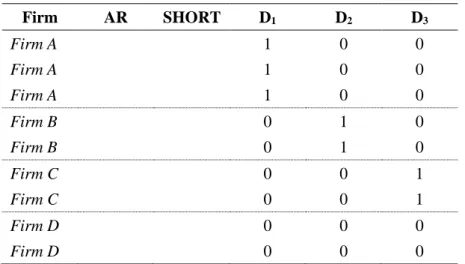
𝐴𝑅𝑖𝑡 = 𝑎0+ 𝛽1𝑆𝐻𝑂𝑅𝑇𝑖𝑡+ 𝐷1+ 𝐷2… 𝐷23+ 𝜀𝑖𝑡 (3.3.1) Where, 𝐴𝑅𝑖𝑡 is the abnormal return of stock 𝑖 at day 𝑡, over a chosen event interval, taking any value in percentages. The independent variable 𝑆𝐻𝑂𝑅𝑇𝑖𝑡 indicates the short positions in percentages of stock 𝑖 at day 𝑡 as it was announced in the registry of FI. At last, 𝛽1 correspond to the coefficient for the variables 𝑆𝐻𝑂𝑅𝑇𝑖𝑡. An example of how we constructed the 23 dummy variables is shown below in Table 1.
12 Six firms were excluded from the sample due to lower short selling activity in percentages (<0.5%), thus, FI has not published short positions for these firms. For more details, see section 3.4.2.
20
Table 1 Example for the formation of LSDV
Firm AR SHORT D1 D2 D3 Firm A 1 0 0 Firm A 1 0 0 Firm A 1 0 0 Firm B 0 1 0 Firm B 0 1 0 Firm C 0 0 1 Firm C 0 0 1 Firm D 0 0 0 Firm D 0 0 0
Note. In this example, 𝐾 = 4, whereas for our sample we have 24 firms (𝐾 = 24), that have been selected for short selling. All 24 firms have been pooled in one panel sepa-rated by 0 and 1 through dummy variables. Notice that the last firm in this example does not have a dummy variable. The last firm is the reference category, determined if 𝐷1 = 𝐷2 = 𝐷3 = 0.
The second model that was used accounts for the multiple announcements of short po-sitions within longer time intervals. Hence, the upcoming model was the second regres-sion model used in this paper. The model stays the same with the only addition of the 𝑀𝑈𝐿𝑇𝐼𝑃𝐿𝐸𝑖𝑡 variable.
𝐴𝑅𝑖𝑡 = 𝑎0+ 𝛽1𝑆𝐻𝑂𝑅𝑇𝑖𝑡+ 𝛽2𝑀𝑈𝐿𝑇𝐼𝑃𝐿𝐸𝑖𝑡+ 𝐷1+ 𝐷2… 𝐷23+ 𝜀𝑖𝑡 (3.3.2) In this case, we have included another independent binary variable to take into consid-eration announcements of new or changed net short position within the longer periods. The variable takes the values of either one or zero. One would indicate a new or a change was announced within a longer time interval, and zero would indicate no announcements of net short positions in a mentioned period. It is important to mention that when FI publishes net short positions, it is already “history” and the market that reads that infor-mation cannot react to it on time. This is also one of the reasons the authors included multiple periods in an attempt to capture the effect of short selling on stock price reac-tions by having enough diversification in time spans.
21
3.4 Data
3.4.1 Data Collection
During the collection of data, multiple sources have been used. Most of the data obtained in this paper are perceived as secondary data, such as government publications or scien-tific articles. The primary sources used in this study for the quantitative part of this the-sis, are Nasdaq OMX Nordic and Finansinspektionen (FI). These sources are to be con-sidered reliable because they are from well-founded institutions.
Regarding net short positions, FI will publish information about a position that reaches 0.5% of the issued share capital and each 0.1% above or below that threshold. Their latest updates state that from the 20th of March 2021, short position holders need to send in notifications only if they reach or exceed the 0.2% threshold again, while they will not have to report an/y outstanding net short position between 0.1% and 0.2%. Also, holders need to notify at each additional 0.1% over and under the 0.2% threshold (FI, 2021).
For the adjusted closing prices, we retrieved and sorted the underlying historical stock prices through Nasdaq OMX Nordic. The time interval that has been selected regarding net short positions is 2017-01-01 to 2020-12-30, while the time interval that has been chosen for the adjusted closing prices of each stock is 2016-12-01 to 2021-01-29. The longer range was necessary to consider the longer event intervals such as (-15,15) on short positions that were announced at the limits of our time interval, i.e., 2020-12-30 or 2017-01-01. All the data solely consist of the adjusted closing prices and net short posi-tions of the thirty most traded stocks that are listed in the OMX Stockholm 30 Index.
3.4.2 Data Adjustments & Sample
Adaptations were made regarding net short positions data in order to make this study feasible. First, in the case where there were multiple net short positions on the same day for a specific stock, we decided to pick only the highest percentage in the hope to record a higher impact on the abnormal returns. Secondly, since we work with a simple panel regression model, we decided to exclude net short positions that were not specified and were published as <0.5%. In addition, six firms were excluded from the sample. The FI has not published any short positions for these firms. However, that does not mean they had zero short positions, it means that they could have been shorted in lower percent-ages, like 0.2%, 0.3%, etc., and FI simply did not publish those short positions. All these
22
limitations could be considered under different econometric models. Models that reckon with censored and truncated data, such as the Tobit model could offer more accurate results. But these techniques are beyond the scope of our skills.
All in all, our initial data contained 30 firms and 2413 observations before adjustments. After the changes, our final sample consisted of a total of 24 firms and 1785 observa-tions. Moreover, for the variable 𝑀𝑈𝐿𝑇𝐼𝑃𝐿𝐸𝑖,𝑡, we have taken into consideration an-nouncements on dates that were outside our time interval for the purpose of accuracy in the data.
23
4 Estimates & Analysis
This section will discuss and provide the estimates from the summary statistics and the empirical findings that originated from the regression analysis described in the method-ology and data section.
4.1 Descriptive Statistics
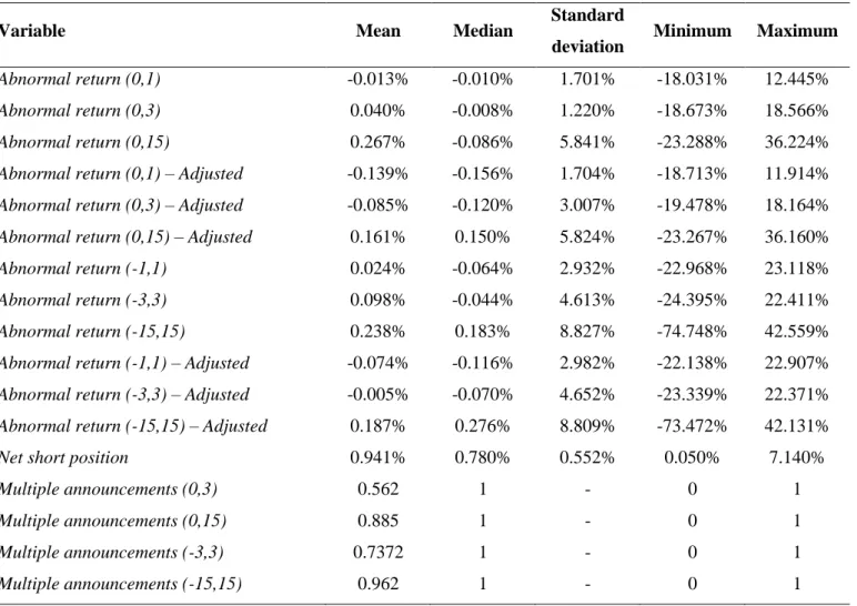
The summary statistics are presented in Table 2 for the response variable and the regres-sors, in our case the main independent variable that records short positions in percent-ages, and the dummy variable which is recorded as binary for multiple announcements within longer periods.
The mean value describes the average value from the sample following the variables. First, we notice that there was no period where the abnormal returns broke away from zero (before the decimals) negatively or positively, implying that abnormal returns were closer to zero for all the periods. These estimates are more in line with studies that found no particular relationship between short selling and stock returns. Next to this, we have the median, which indicates the value situated in the middle of the data set. Once more, even though the negative symbol prevails, we see that in none of the periods the abnor-mal returns escape from zero (before the deciabnor-mals).
The table also shows us the standard deviation which demonstrates an estimate for the appearance of extreme values. Extreme values are considered those that are far away from the mean. We observe that the values of standard deviation for all periods are sat-isfying, meaning that they are relatively low and the abnormal returns for each period are close to the mean of our data set. Thus, there is no need to create another dataset to exclude extreme outliers to increase standard deviation efficiency. Finally, the satisfac-tory standard deviations can also be spotted from the minimum and maximum columns. There are no extreme values except for the longest period (-15,15) for both adjusted and non-adjusted abnormal returns which has a maximum and minimum value slightly higher than usual, -74.748% and 42.559% for non-adjusted and -73.472% to 42.131% for adjusted abnormal returns. Regarding our categorical variable, the mean for the pe-riod (0,3) is 0.562, while as we move on to the longer pepe-riods, this number increases. This is reasonable since there are more opportunities for short sellers to short shares
24
within a longer time window. Lastly, the average of net short positions is 0.941%, rang-ing from 0.050% to 7.140%.
Table 2 Descriptive Statistics
Variable Mean Median Standard
deviation Minimum Maximum
Abnormal return (0,1) -0.013% -0.010% 1.701% -18.031% 12.445%
Abnormal return (0,3) 0.040% -0.008% 1.220% -18.673% 18.566%
Abnormal return (0,15) 0.267% -0.086% 5.841% -23.288% 36.224%
Abnormal return (0,1) – Adjusted -0.139% -0.156% 1.704% -18.713% 11.914% Abnormal return (0,3) – Adjusted -0.085% -0.120% 3.007% -19.478% 18.164%
Abnormal return (0,15) – Adjusted 0.161% 0.150% 5.824% -23.267% 36.160%
Abnormal return (-1,1) 0.024% -0.064% 2.932% -22.968% 23.118%
Abnormal return (-3,3) 0.098% -0.044% 4.613% -24.395% 22.411%
Abnormal return (-15,15) 0.238% 0.183% 8.827% -74.748% 42.559%
Abnormal return (-1,1) – Adjusted -0.074% -0.116% 2.982% -22.138% 22.907% Abnormal return (-3,3) – Adjusted -0.005% -0.070% 4.652% -23.339% 22.371% Abnormal return (-15,15) – Adjusted 0.187% 0.276% 8.809% -73.472% 42.131%
Net short position 0.941% 0.780% 0.552% 0.050% 7.140%
Multiple announcements (0,3) 0.562 1 - 0 1
Multiple announcements (0,15) 0.885 1 - 0 1
Multiple announcements (-3,3) 0.7372 1 - 0 1
Multiple announcements (-15,15) 0.962 1 - 0 1
Note. The variables are shown in the rows and the summary statistics in the columns.
Decimals numbers are rounded to three decimals.
4.2 Regression Estimates
We ran twelve regression analysis to account for all the periods that were chosen from section 3.1. The results are put forward in and Table 4 where the values of the coeffi-cients for each variable are marked in the rows, while the columns designate the periods for both adjusted and non-adjusted abnormal returns.
The results are closer to previous studies such as Woolridge, (1994), which stated there is no significant relationship between net short positions and stock returns, i.e., a high level of short interest is not necessarily a bullish or bearish indicator. Additionally, short
25
sellers did not always earn excess returns on their investment. We found that abnormal returns are not more negative when there is a higher level of net short positions. That would also mean that short sellers do not possess superior information in order to take advantage of easy profits. Although our study focuses only on 24 companies from the Swedish market, these companies have the highest trading volume in the market and that could lead to potential weighty estimates and results.
4.2.1 Periods (0,t)
The results for periods (0,1), (0,3), and (0,15) are shown in Table 3. In this table, we have run six regressions to examine adjusted and non-adjusted abnormal returns for the periods that include the day of the announcement and a certain day after the announce-ment.
4.2.1.1 Abnormal Returns
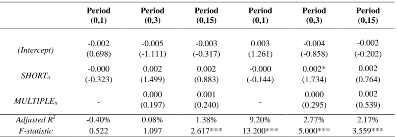
To assess the reliability of the model, we can examine the adjusted R-squared and F statistic. Adjusted R squared indicates to what degree the variation of the dependent variable is explained by the independent variables. We see that adjusted R-squared is relatively low and even negative for the period (0,1). Our model seems to not be signif-icant for periods (0,1) and (0,3) as the F statistic is not signifsignif-icant. Though, in period (0,15), approximately 1.53% of the variation in abnormal returns can be explained by the short position announcements. Also, the F statistic in that period is significant with a P-value below 0.01. However, we found that none of the coefficients is statistically significant apart from the period (0,3), where our key independent variable 𝑆𝐻𝑂𝑅𝑇𝑖𝑡 is significant at 0.05 level. For that period, the model predicts that the value of the inde-pendent variable increases by 0.003 for every one-unit change in the predictor. That shows a slight profit loss for the short sellers; therefore, it would imply that the result is more aligned with studies that support short sellers are not informed.
4.2.1.2 Adjusted Abnormal Returns
Things are somewhat different when considering the adjusted abnormal returns. Our model seems to be significant for all the periods with P-value below 0.001 and 0.01. However, we find that none of the coefficients was statistically significant apart from the period (0,3), again for the net short positions variable which takes the same value as the non-adjusted abnormal return in period (0,3). Also, for the period (0,1), adjusted R-squared and F statistic are polar opposite in comparison to the non-adjusted abnormal
26
return for the same period. Adjusted R-squared takes the value of 7.89% with significant F at the 0.001 level.
Table 3 Regression results for Periods (0,1), (0,3), and (0,15)
Abnormal Returns Abnormal returns – Adjusted
Period (0,1) Period (0,3) Period (0,15) Period (0,1) Period (0,3) Period (0,15) (Intercept) (-0.145) -0.000 (-0.972) -0.005 (-0.451) -0.001 (1.625) 0.004 (-0.200) -0.001 (-0.040) 0.000 SHORTit (0.992) 0.001 (1.894) 0.003* (0.737) 0.002 (1.093) 0.001 (2.011) 0.003* (0.159) 0.000 MULTIPLEit - (0.499) 0.001 (0.186) 0.001 - (0.517) 0.001 (0.494) 0.002 Adjusted R2 -0.63% 0.32% 1.53% 7.89% 2.77% 1.27% F-statistic 0.517 1.234 2.147** 7.612*** 3.109*** 1.949**
Note. The periods are shown in the columns, whereas the values of each of the variables
in the models are depicted in the rows. The number enclosed in brackets displays the result of the t-test, whereas the coefficient of each variable is directly overhead. At the bottom, we also have the adjusted R2 and the F-statistic for every model, (N = 1,785).
Table 4 Regression results for Periods (-1,1), (-3,3), (-15,15)
Abnormal Returns Abnormal returns – Adjusted
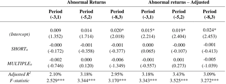
Period (-1,1) Period (-3,3) Period (-15,15) Period (-1,1) Period (-3,3) Period (-15,15) (Intercept) (0.754) 0.004 (0.676) 0.005 (0.197) 0.003 (1.800) 0.009• (1.353) 0.010 (0.389) 0.007 SHORTit (0.177) 0.000 (0.748) 0.002 (0.661) 0.003 (0.429) 0.001 (0.977) 0.002 (-0.014) -0.000 MULTIPLEit - -0.001 0.010 - -0.001 0.014 (-0.492) (0.864) (-0.335) (1.156) Adjusted R2 0.67% 1.49% 4.03% 4.90% 1.87% 3.49% F-statistic 1.521* 2.122*** 4.105*** 6.093*** 2.408*** 3.672***
Note. The estimates are structured in the same way as Table 3. However, in this table,
the models include the dates prior to the announcement of a short position, (N = 1,785).
27
4.2.2 Periods (-t,t)
The results for period (-1,1), (-3,3), and (-15,15) are presented in Table 4. In this table, the regression analysis considers the days prior to the announcement of short positions.
4.2.2.1 Abnormal Returns
For the periods (-1,1), (-3,3), and (-15,15), once again the coefficients appear to take values close to zero. Yet, none of the independent variables is statistically significant. However, the model is significant for all three periods, with the highlight being the longer period (-15,15). Approximately, 4.03% of the variation of abnormal returns is explained by the coefficients, and the model for the period (-15,15) is significant at the 0.001 level with an F value of 2.147. So far, we do not have enough evidence to support the hypothesis from prior studies that short selling influences stock returns negatively.
4.2.2.2 Adjusted Abnormal Returns
For the periods (-1,1), (-3,3), and (-15,15), the regression models which include the ad-justed abnormal returns yield similar results with the models for the unadad-justed abnor-mal returns. We repeatedly find that there is no statistical significance among the coef-ficients. The F statistic takes satisfactory values again with P-values below 0.001 in pe-riods (-1,1), (-3,3), and (-15,15). We notice a slightly similar pattern in regard to the model fit for the adjusted abnormal returns in periods (0,1), (0,3), and (0,15). Given that none of the coefficients is statistically significant, once more we find no evidence that short selling has a negative impact on stock returns. Overall, we have consistently found that there is not enough evidence that shows a particular relationship between short sell-ing and stock returns in the Swedish market.
28
5 Conclusion
It is relatively clear that the consensus among most researchers is that short selling is healthy for the market, as it helps to “regulate” in a way overvalued securities. Also, a lot of studies found that banning short selling led to a decrease in market efficiency. However, many researchers want to investigate how transparent and exploitable short selling is by examining abnormal returns in connection to short selling.
The expectations were based on a hypothesis that has been raised by many researchers. Does short selling negatively impact stock returns? Although many studies have found a strong negative relationship between short selling and stock returns, some studies also found no significant relationship like Woolridge, (1994). Our results are closer to the latter. The results we found were not in line with previous literature such as Diamond and Verrechia, (1987) and Figlewski et al., (1993), which supported the notion that an increase of short interest in a stock leads to negative price reactions. In our study, we did not find enough evidence to support the hypothesis stated in section 2.3. Even though the model fits were significant for almost all the periods, none of the coefficients was statistically significant apart from the period (0,3) where the coefficient of short posi-tions for both adjusted and non-adjusted abnormal returns was not in the expected direc-tion. It was positive but nearly zero. This implies that a higher level of short positions did not lead to excess returns. From these results, we could infer that investors in the Swedish market do not possess private information that could generate unfair profits. Considering the limitations of this thesis, we could not draw direct conclusions. There-fore, this leaves room for repetition of this study, which includes more variables in the regression model in an attempt to eliminate any reasonable bias.
29
6 Limitations & Recommendations for
Future Research
This paper does not include two variables in the regression models that could potentially shift the results. Prior research has used both the optioned and tax variable. For instance, they found that optioned stocks make short selling easier in multiple ways (Figlewski et al.,1993). Also, it is recommended to consider other events that happened close to the announcement dates. Such events could have potentially influenced the abnormal returns and the nature of its relationship with short selling.
Other studies have utilized different data, such as short interest as well as high frequency and daily data within a specific index, whereas, in our paper, short selling data was ob-tained through net short positions announced in the Swedish registry (FI). It is worth mentioning that the numbers of net short positions are multidimensional, and we did not account for the duration of the short selling, i.e. when short sellers closed their positions. For the extended periods, we did not average short positions that occurred on the same firm, we considered each number separately. A closer look into the extended periods could offer an interesting addition to the study. Besides that, an issue that arises with announcements of net short positions is that there is some lag. The announcements do not represent the true timing of the short selling. Usually, it takes some time until short selling appears in the registry. Hence, there could be a bias towards whether short sellers are informed or uninformed. For that reason, a deeper look into information asymmetry within perhaps different sizes of firms regarding short selling would be exciting for fur-ther studies.
A possible explanation for not finding any negative relationship between short selling and stock returns for the long buyers is that short sellers bought the shares back relatively fast, meaning that our periods did not accurately capture the effect. Consequently, as mentioned earlier, a study that gathers data for closed positions from short sellers would be worthwhile for future research, or it would be also effective if one could estimate the duration of the short selling and see the opposite effect when they bought back the shorted shares.
To test further the hypothesis, someone could supplement the analysis with a different calculation of abnormal returns. The computations in chapter 3.2.1 were done for each
30
date separately. With this method, there is a degree of uncertainty on the results, since big fluctuations in stock price may not be captured accurately among the longer periods. Hence, future studies could calculate cumulative abnormal returns (CAR)13. Addition-ally, since six firms were excluded from the sample, it would be also interesting to com-pare the abnormal returns with the value-weighted index of OMXS30, i.e., not the equal-weighted index.
Moreover, the computation for the adjusted abnormal returns has its limitations. There-fore, it would be sensible to try different methods to adjust risk in excess returns. Lastly, the setup of this study has been confined to a time interval and only for the Swedish setting. Conclusions cannot be drawn for other financial markets or other time intervals.
13 With the CAR method, we essentially add all the sums of the abnormal returns through a specific time interval. In other words, it is the aggregated abnormal return for a stock at a specific date.