A net dose model for development of nausea

A net dosemodel for development

of nausea

Paper presented at the 34th United Kingdom Group Meeting

on Human Responses to Vibration, held at Ford Motor

Company, Dunton, Essex, England, 22-24 September 1999

c» as 05 '_'-l O

co

oo

x 0 >. a. H 5. 3GB 01

Björn Kufver and Johan Förstberg

Comparison between the net dose model and nausea ratings

Simulator study 1998. 44 subjects on their first test mn. Mean values 2

NR = 0 No symptoms I 1 8 __ NR = 1 Light symptoms but no + NR Female (N=23)

nausea . _{+ NR Total (N=44)} NR = 2 ngh'l nausea » * NR=3Moderate nausea t 1,4 / A ___ \\ 1,2 / m \\

//// A __ \\

0,8 %),/fx \\

_%

_\

_V. 0,6

/ Total Male Female

0,4 cAA/cL 1,53 1,02 1,97 + NR Male (N=21) Na us ea ra ti ng s (N R)

- Time when subjects

1/cL 12,5 11,2 13,1 [mm] _ ,

0,2 _ Do -0,01 -0,06 0,04 estimated therr NR 0 Stop ol motion (31 min)

0 5 10 15 20 25 30 35 40 45 _ Time [min]

Swedish NationalRoad and ;

VTI särtryck 330 ' 1999

A net dose model for development

ofnausea

Paper presented at the 34th United Kingdom Group Meeting

on Human Responses to Vibration, held at Ford Motor

Company, Dunton, Essex, England, 22 24 September 1999

Björn Kufver and Johan Förstberg

edisir :

:

ISSN 1102-626X

A net dose model for development of nausea

Björn Kufver and Johan Förstberg

Railway Systems

Swedish National Road and Transport Research Institute (VTI)

SE- 581 95 Linköping Sweden

e-mail: bjorn.kufver©vti.se, johan.forstberg©vti.se

Abstract

For prediction of nausea among travellers in a tilting train running at different possible speed levels and on different types of alignments, the following characteristics of the time dependency of a model are highly desired. During provoking but stationary conditions, nausea should be increasing with time, but with a declining rate of change (according to previously published data from various authors). The model should be able to deal with non-stationary conditions (such as a mixture of alignment characteristics for the train, i.e. straight lines and

curvaceous lines). The model should be able to predict the decline of nausea

during rest after a provoking exposure of motions.

This paper is focused on the time dependency in such a model. The influence of

frequencies and directions (longitudinal, lateral, vertical, roll, yaw, pitch) of motions are not in focus.

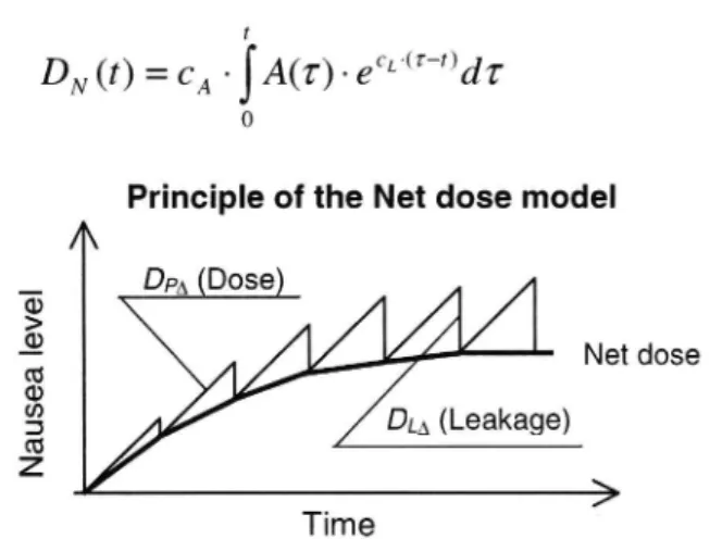
A new model is based on the following assumptions. . Nausea is linearly dependent to a net dose, DN(t).

. During a short time interval dt, two processes affect the magnitude of the net dose.

. An increase of the net dose is proportional to the amplitude A(t) of motion during the time interval.

. Leakage, which is always present, is proportional to instantaneous net dose.

This means that the net dose at time t+dr may be calculated as DN(t+dr) = DN(t) + 0,4 A(t) dt cL D,,(t)- dr

where CA and CL are constants, tis time and dr is time step. The expression may be

rearranged as

!

DN (t) = c,, - j A(r) . eCL' _ dz'

0

Various characteristics of this function and curve fitting to survey data are presented and discussed.

Keywords

Nausea, Time dependency, Non-stationary, Exposure, Recovery, Threshold value.

Presented at the 34th United Kingdom Group Meeting on Human Responses to Vibration, held at Ford

1 Introduction

When travelling, motion sickness is sometimes an unpleasant and unwelcome side-product of motions

or moving visual fields. Some people are highly susceptible but other hardly notice any kind of symptoms. With the introduction of tilting trains, running at higher speeds than conventional trains on curvaceous lines, motion sickness has become a problem for some of the train passengers (Förstberg,

Andersson, & Ledin, 1998; ORE, 1985).

Tilting trains run partly on new lines with a high geometric standard (straight lines, circular curves with large radii, long transition curves between straight lines and circular curves) and partly on old lines

with a low geometrical standard (circular curves with small radii and short transition curves). Hence, a

model that can predict motion sickness should include influence not only of various types of motions (vertical, lateral, roll, etc.), different frequencies but also non-stationary conditions. Hence, the time dependency of such a model is crucial.

2

Existing models for prediction of nausea and motion sickness

There are two different groups of models to predict nausea and motion sickness: Descriptive models and functional models (Bos & Bles, 1997). The descriptive models are mathematical functions fitted to experimental data, where motion sickness depends on quantities of the provoking motion (e.g.

acceleration magnitude, frequency and duration). Functional models are based on the conflict theory and take characteristics of the vestibular system into account.

An investigation of earlier models for prediction of nausea and motion sickness shows that the models

from McCauley et al (McCauley, Royal, & Wylie, 1976) and Lawther and Griffin s motion dose model (Griffin, 1990; Lawther & Griffin, 1987) are the most commonly used ones. McCauley s model is mathematically complicated and Lawther and Griffin s model is rather simple. The motion dose model

has now become an international standard for prediction of Motion Sickness Incidence (MSI) from

vertical accelerations (ISO, 1997). Both these models are of the descriptive type.

Time dependency. With a fixed frequency and amplitude of the provocative input the motion sickness incidence1 (MSI) will rise with time taccording to:

MS] = k . (I: (log t) McCauley et al s model [1]

where (P( ) is the standardised normal distribution function

MSI = k ~ x/t Lawther and Griffin s model2 [2]

1 Motion Sickness lncidence (MSI) or Vomiting Incidence (VI) O 100%.

The time dependency of the model of McCauley et al is the following: The first derivative of MSI is

positive. For small values of exposure time t, the second derivative of MSI is positive. For larger values

of t, the second derivative of MSI is negative and converges to zero when tgoes to infinity. The MSI function then converges to a constant level. The model refers to exposures of motions with constant

amplitude. This is a major drawback in the applications with tilting trains.

The time dependency of Lawther and Griffin's model is the following: The first derivative of MSI is

positive and the second derivative is negative. The model is restricted to exposures less than 6 hours. Their original model can cope with variable amplitudes.

Functional models have been presented by Oman (1982, 1990) and Bos & Bes (1997, 1998) and will

not be further discussed in this paper.

3 The net dose model

A new model, the net dose model, was developed based on the assumption that nausea is correlated to the net dose of motion DN, defined as the difference between the perceived dose Dp and the

accumulated leakage DL.

The model is aimed only to explain the time dependency. Directions of motion (longitudinal, lateral,

vertical, roll, pitch, and yaw) and frequencies are assumed to be constant during the exposure. Hence,

the provocative motion may be described by a constant amplitude A (or variable amplitude A(t), when amplitude varies with time t).

The perceived dose during a certain exposure time is assumed to be proportional to the product of amplitude A and exposure time At,

DPA = cA A At [3]

or

D%=mAmAt _[M

if amplitude A(t) is approximately constant during the exposure time At.

The leakage DLA during a time interval At is assumed to be proportional to the accumulated net dose DN at the beginning of the interval,

DLA = cL-DN(t)-At [5]

Hence, for an infinitesimally small time interval dr the change of net dose DN may be expressed as

dDN = DN(t+dr) - DN(t) = cA A(t)-dr - cL DN(t).dr [6]

Integrating [6] from an early start (7:0) leads to the general formula

t

DN (t) = CA - j Am - en dr

[7]

O

Principle of the Net dose model

A _ DPA Dose (1) > 9 Net dose

$

% DLA (Leakage) Z \ / Time '

Figure 1 Principle of the net dose mode/. The dose is increased by the amount DPA and decreased by amount DLA.

Some observations may be done of the behaviour of this net dose function. 3.1 Start of exposure at experiment

Assume the actual net dose is approximately nil at the start of an experiment (where t=ts) and the

motion amplitude during the experiment is constant at the level A.

The net dose may than be expressed as

cA A DN (0 = CA ' A IfM dr = S

-(1 e CL " >

[81

C L ts<_ts_te

ts = start of experiment, te = end of experiment

This function has a negative second derivative (with respect to time) and should be able to suit data

that previously have been used in curve fittings where time derivative is negative (functions [1] and

[2])-It should also be noticed that function [7] (and hence also [8]) does not increase infinitely with

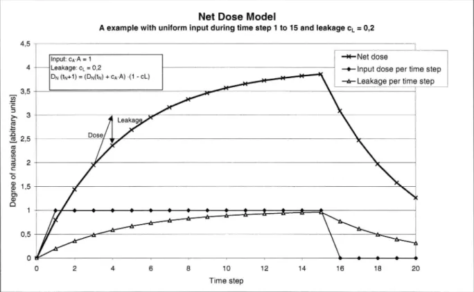
increasing time as a dose function related to the square root of time does. The need for a restriction in exposure time t is therefore eliminated. The shape of the function during exposure to constant amplitude is shown in the left part of Figure 2.

Net Dose Model

A example with uniform input during time step 1 to 15 and leakage c,_ = 0,2

,3

/

_\

4,5 _i

Input: cA-A = 1 *Net dose

4 Leakage: cL = 0,2 _o lnput dose per time step 3 5 25 Dose

/ V

/

\

\

X

De gr ee of na us ea [a bi tr ar y un it s]

\<

%

\

*

O » i i - = é : O 2 4 6 8 10 12 14 16 18 20 Time step

Figure 2 Example of net dose model - exposure with fixed amplitude (left) and recovery period (right).

3.2 End of exposure

Assume that a dose DNe has been achieved at the end of the exposure time te

cA-A

DN. =DNir.) =

.(1__

e W- p

CL

If no further exposure is made, a pure leakage will appear

DN (t) : DNe 'Jag te) läte

See the right part of Figure 2.

3.3 Test of the net dose model

Estimation of the leakage factor CL based on data collected during exposure (according to [8]) should

be compared with an estimation of cL based on data collected after exposure (according to [10]). If the assumptions above are correct, CL should remain the same in all cases.

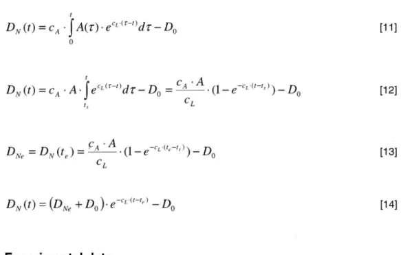
3.4 Threshold values

Normally, it takes some time before subjects show some degree of nausea. This may be explained by

a time threshold (McCauley et al., 1976). Applied on the net dose model,

[9]

[10]

it seems more reasonable to

DN (t) = CA - ] A(r) . eCL' _t)dr D0

[11]

O !

A

DN (1) = CA - A - ] fdr dr D0 = CA » (1 en ts) ) D0

[12]

ts CL

DM, = DN(te) = CA -(1 e"cr< e f~v>) DO

[13]

CL

DN (t) = (Dive + Do )- fw ) Do

[141

4

Experimental data

The net dose model has been fitted to data from different experiments. The first example (Figure 3) shows nausea ratings as averages from 19, 25 and 44 test subjects in a simulator test at VTI, Linköping, Sweden, where subjects were exposed to lateral and roll motions (Förstberg, 1999). The

motions were cyclical with a period of 1 minute. A recovery period starts at the 31St minute. (Since the

answers at the start of the recovery period were somewhat delayed, they are plotted at minute 32.)

Comparison between the net dose model and nausea ratings

Simulator study 1998. 44 subjects on their first test run. Mean values 2

NR : 0 No symptoms i 1 8 __ NR : 1 Light symptoms but no - A NR Female (N=23)

rlllalztjseza L- ht _{+NR Total (N=44)}

= lg nausea Ä (& _

1,6 __ NR = 3 Moderate nausea / \\ +NR Male (N 21)

1,4 A A -L "M

/mx

///// A, XX

MÅXX

Na us ea ra ti ng s (N R) 0,8 _\\A 0,6

/

Total Male Female

\

0,4 GAA/CL 1,53 1,02 1,97 _ .

1/c._ 12,5 11,2 13,1 [min] Te 1111315111115? 02 D0 -o,o1 -0,06 0,04 95 "a e e"

0 Stop of motion (31 min)

0 5 10 15 20 25 30 35 40 45

Time [min]

Figure 3 Average responses from 44 different subjects and a fit of the net dose model to

these data. Data were sampled each 5 min with start at 1 min after start of test run.

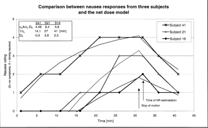
Figure4 shows ratings on individual basis from the same experiment. The large differences in

individual threshold doses Do should be noted.

Comparison between nausea responses from three subjects and the net dose model

5 S41 821 S16 . cAA/cL-Do 4,46 6,4 5,6 +Sub1ect41 1/c,_ 14,1 27 41 [min] wSubjetht 4 __D() -o,5 3,8 2,5 +Subject 16 a 83 = 2 U) ? 5 3 två 175 h ll (U v 3 o 2 % 2 / a 8 / M Å & T 1 / A V + | v \v! Time of NR estimatation Stop of motion O A A i _ , l, O 5 10 15 20 25 30 35 40 45 Time [min]

Figure 4 Responses from 3 different subjects and a fit of the net dose model to these data. Data were sampled each 5 min with start at 1 min after start of test run. Source: Simulator experiment done by Förstberg (1999).

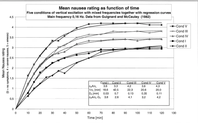
The third example is from an experiment done by Guignard and McCauley (1982), see Figure 5. They

tested five different combinations of vertical accelerations. The provocative excitation was rather

strong, with vertical accelerations of 1,3 m/s2 r.m.s. at a frequency of 0,17 Hz combined with

frequencies of 0,33 or 0,5 Hz. After 2 h conditions l and ll had 50% MSI and condition V had 78% MSI.

No recovery data are published. The model fits the data rather well.

The fourth example is from an experiment done by Golding & Kerguelen (1992) with lateral or vertical

accelerations, see Figure 6. Here the provocative excitations are of the same magnitude but with a higher frequency than the previous experiment (1,8 m/s2 r.m.s. at a frequency of 0,3 Hz). These

authors have published recovery data, but the leakage factor cL of the excitation period (up to 45 min) were not estimated to be the same as in the recovery period (45 55 min).

Mean nausea rating as function of time

Five conditions of vertical excitation with mixed frequencies together with regression curves 4,5 Main frequency 0,16 Hz. Data from Guignard and McCauIey (1982) T

4 +Cond V A -N-~Cond III % 3,5 -Ar~Cond IV (is? +Cond I 3 3 +Cond II c) (15 E 8

a

g 9 2,5 CU co

"få :: 2

_{$ 2}

2 gts

% C n l n II n I n IV n V % GAA/CL 3,6 3,3 4,2 3,6 4,3 C") 1 1/cL [min] 18,6 42,5 22,3 20,6 20,0 " V Do [min] 0,03 0,7 0,13 0,35 0,11 0 5 cAA/cL-Do 3,6 2,6 4,1 3,2 4,2 _ O I | I I I I I ' I I I I 0 10 20 30 40 50 60 70 80 90 100 1 10 120 130 Time [min]

Figure 5 Net dose model - curve fitting to experiment by Guignard and MoCau/ey (1982).

Mean sickness

According to Golding and Kerguelen experiment 1992

7 _ Golding and Kerguelen sickness scale

(adjusted): ? o = No symptoms

~ -x-V t

q, 1 = Any symptoms however slight er eyes

g 6 " 2 = Mild symptom & M opened

95 3 = Mild nausea -A- Vert eyes

Q g = miiccij to moderate nbausea closed

= o erate nausea ut can continue .

% 5 __ 6 = Moderate nausea and wish to stop + Horlz eyes

c» opened % + Horiz eyes 5 4 _ closed (5 o' 0 (U CD E 3 _' O 4

ea

_{'; . . .}

.,

I

_\ .E 2 _ ' - v v

E

_(,,

x f

_,

»» " * v

' '

6

f?

'

£ 1 _ (y'/"l .] g ./ / w // _ _*.'/'_ . NNK O I I... I 1 1 1 ! Y T , ' 'N' 3" _ I 0 5 10 15 20 25 30 35 40 45 50 55 Time [min]

5 Analysis and discussion

The potential benefit of with the net dose model is the ability to cope with non-stationary conditions in

the motions, combined with fewer restrictions for the evaluation period.

In certain cases, a good agreement was found between data and model. However, in other cases,

such as using data from Golding and Kerguelen, the model showed poor agreement with data. In this case, estimations of the CL give significantly different values for the exposure period and the recovery period, respectively. Introducing two different Ieakage factors for these two cases may lead to the need of many different Ieakage factors for motions with different severity, and the foundation for the model is eroded.

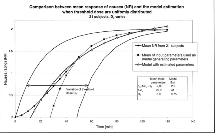
One reason for poor agreement between the model and mean ratings is the fact that registered zero values for sickness ratings sometimes need to be modelled as negative values (ratings in the interval between -D0 and zero). Figure 7 illustrates the consequences in an example where the acceleration

amplitude A is constant, and where the CL is the same for the different individuals. The threshold dose

Do is assumed to vary between different individuals.

Comparison between mean response of nausea (NR) and the model estimation when threshold dose are unifomly distributed

21 subjects, Do varies

+Mean NR from 21 subjects

1

m... Mean of input parameters used as medel generating parameters war-Model with estimated parameters 1

Mean Input Model

x parameters Est /\ / CA A/CL 'Do 2,00 2,2 0 5 % / Variation of thr hold 1/(3L 20,0 41 1 DO 5,8 0,75 __ 0 ' | / I / I l l 20 4 dose Do O 60 80 100 120 140 Time [min] 1,5 Na us ea ra ti ng s (N R)

Figure 7 Comparison between the mean response from 21 subjects with varied threshold doses Do and model estimation. Other parameters are constant.

ln Figure 7, the threshold dose Do varies uniformly and with a Ieakage factor CL of 1/20 min'1. However,

the mean of the 21 subjects responses is not the same as the response model from the mean of the

subjects will underestimate the leakage factor. (The mean of subjects nausea ratings also shows a positive second derivative for short exposure time t, as a consequence of neglecting the interval

between -Do and zero.)

This may be the explanation for the differences in leakage factors from the experiment from Golding & Kerguelen (1992), where the leakage constants during excitation is lower than the leakage constants during the recovery period.

Conclusions

The net dose model seems to have the potential to explain the individual responses to provoking stimuli. The modelling of a response from a group of subjects tends to lead to different estimations of

leakage factors for provocation and recovery, unless the model is refined. The potential advantage of

the model is the ability to cope with varying amplitudes of provoking inputs and to longer exposures

than 6 hours.

Acknowledgements

This project is financed by Adtranz Sweden, the Swedish State Railways (SJ), the Swedish Transport

and Communications Research Board (KFB) and the Swedish National Road and Transport Research

Institute (VTI) and we are very grateful for helpful co-operation and contributions from them.

References

Bos, J. E., & Bles, W. (1997). A vestibular-based motion sickness incidence model (Report TM-97-A032). Soesterberg: TNO Human Factors Research Institute.

Bos, J. E., & Bles, W. (1998). Modelling motion sickness and subjective vertical mismatch detailed for vertical motions. Brain Res Bull, 47(5), 537-42.

Förstberg, J. (1999). Effects from lateral and/or roll motion on nausea on test subjects: Studies in a

moving vehicle simulator. Paper presented at the 34th UK group meeting on human responses

to vibration, held at Ford Motor Company, Dunton, (Essex, England), 22 -24 Sept. 1999, Dunton (England).

Förstberg, J., Andersson, E., & Ledin, T. (1998). The influence of roll acceleration motion dose on travel sickness: Study on a tilting train. Paper presented at the 33rd meeting of the UK group on human response to vibration, 16th - 18th Sept. 1998, Buxton (England).

Golding, J. F., & Kerguelen, M. A. (1992). A comparison of nauseogenic potential of low-frequency

vertical versus horizontal linear oscillation. Aviation, Space, and Environmental Medicine, 63,

491-497.

Griffin, M. J. (1990). Handbook of Human Vibration. London: Academic Press.

Guignard, J. C., & McCauley, M. E. (1982). Motion sickness incidence induced by complex periodic

waveforms. Aviation, Space, and Environmental Medicine, 554-563.

ISO. (1997). Mechanical vibration and shock - Evaluation of human exposure to whole body vibrations

- Part 1: General requirements (ISO 2631-1.2:1997 (E)). Geneva: ISO.

Lawther, A., & Griffin, M. J. (1987). Prediction of the incidence of motion sickness from the magnitude, frequency, and duration of vertical oscillation. Journal of Acoustical Society of America, 82(3), 957-966.

McCauley, M. E., Royal, J. W., & Wylie, C. D. (1976). Motion sickness incidence: Exploratory studies of habituation, pitch and roll, and the refinement of a mathematical model (Technical Report, No 1733-2, AD-AOZ4 709). Goleta (California): Human Factors Research Inc.

Oman, C. M. (1982). A heuristic mathematical model for the dynamics of sensory conflict and motion sickness. Acta Otolaryngol Suppl, 392, 1-44.

Oman, C. M. (1990). Motion sickness: a synthesis and evaluation of the sensory conflict theory. Canadian Journal of Physiology and Pharmacology, 68(2), 294-303.

ORE. (1985). Body tilt coaches - Operational experience with body tilt coaches (BT) (ORE $1037 Rp1). Utrecht: ORE (ERRl).