Oil and the 'Dutch Disease' : - The Case of the United Arab Emirates

J

I

B

S

Oil and the ‘Dutch Disease’

-

The Case of the United Arab Emirates

Bachelor Thesis within Economics

Author: Maxine Eden 840504 Johanna Kärnström 840616 Tutor: Professor Per-Olof Bjuggren

Ph.D Candidate Andreas Högberg Ph.D Candidate Erik Åsberg Jönköping January 2009

Bachelor Thesis within Economics

Title:

- The Case of the United Arab Emirates

Authors: Maxine Eden 840504

Johanna Kärnström 840616

Tutors: Per-Olof Bjuggren

Andreas Högberg

Erik Åsberg

Date: 2009-01-26

Keywords: Dutch Disease, Non-tradable Goods, Resource Movement Effect, Spending Effect, Tradable Goods, United Arab Emirates.

JEL Classifications: E31, N55, O13

Abstract

According to the Dutch Disease core model a boom in natural resources will eventually lead to a shift of production between sectors: from tradable goods to non-tradable goods. The authors found it interesting to research if United Arab Emirates has been a subject to any of the effects caused by the disease, due to the oil boom during the 1970s and the huge development that has appeared in the country. If the United Arab Emirates would be a vic-tim of the disease the decline in exports of the natural resource will result in a decline in the non-oil tradable goods which will affect the country negatively. Furthermore, the disease can also make it more difficult for the country to deal with the problem of high inflation. A time series covering the period 1975-2005 is used to analyse if the United Arab Emirates has experienced symptoms of the disease. Results show that the country has experienced some symptoms of the Dutch Disease during the period 1975-198 since changes in the price of oil caused tradables to shift to the non-tradable sector. Another sign of the disease is the high inflation rate Unite Arab Emirates experienced during the selected period, how-ever high inflation rate could be caused by other factors as well. Furthermore, the larger in-crease in the non-tradable sector compared to the tradable sector is also an indication of the disease in the country. According to these findings the authors can conclude that United Arab Emirates has experienced symptoms of the disease, however, it cannot be concluded that it has been a victim of the disease.

Kandidatuppsats inom Nationalekonomi

Titel: Olja och holländska sjukan - Fallet Förenade Arabemiraten

Författare: Maxine Eden 840504

Johanna Kärnström 840616

Handledare: Per-Olof Bjuggren

Andreas Högberg

Erik Åsberg

Datum: 2009-01-26

Nyckelord: Effekten av fördelning av tillgångar, effekten av utgifter, Förenade Arab Emiraten, handelsvaror, holländska sjukan, icke handelsvaror.

JEL-koder: E31, N55, O13

Sammanfattning:

Enligt holländska sjukan-modellen kan en plötslig boom inom naturtillgångar leda till en förskjutning av produktion mellan sektorer, från handelsvaror till icke handelsvaror. Syftet med denna kandidatuppsats är att undersöka om Förenade Arabemiraten har varit ett offer för sjukan på grund av den oförväntade ökningen av naturtillgångar som skedde i landet under 1970-talet. Landet skulle påverkas negativt om det var ett offer för sjukan då nedgången i oljeexporten skulle resultera i en nedgång i sektorn för icke-olje handelsvaror. Detta i sin tur skulle påverka landets BNP negativt. Ytterligare ett problem som Förenade Arabemiraten skulle uppleva om landet är ett offer för sjukan, är svårigheter att kontrollera den höga inflationen. En tidsserieanalys för perioden 1975-2005 användes för att undersöka om ökningen av naturtillgångar ledde till symptom av sjukan. Under perioden 1975-1980 påverkades landet av förändringen i oljepriset vilket ledde till att handelsvaror skiftade till sektorn för icke handelsvaror, vilket är ett av symptomen för den holländska sjukan. Andra indikationer på att sjukan har förekommit under den testade perioden, är den höga inflationen. Dock kan inflationen ha påverkats av andra faktorer som till exempel den fasta växelkursen till den amerikanska dollarn. Under perioden 1975-2005 har sektorn för icke handelsvaror ökat dubbelt så mycket som sektorn för handelsvaror, detta är ytterligare ett symptom av sjukan. Enligt de resultat författarna erhållit kan det konstateras att Förenade Arabemiraten har påvisat symptom av sjukan, däremot kan det inte konstateras att landet har varit ett offer för sjukan på grund av att andra faktorer kan ha påverkat och orsakat de symptom som landet upplevt.

Table of Contents

1

Introduction ... 1

1.1 Purpose... 2

1.2 Outline... 2

2

U.A.E Background and Previous Studies ... 3

3

Theoretical Framework ... 5

3.1 The TNT Model ... 5

3.2 The Dutch Disease Models ... 6

3.3 The Corden and Neary Core Model ... 7

3.3.1 The Spending Effect ... 7

3.3.2 The Resource Movement Effect ... 8

3.4 Dutch Disease - Sachs and Larrain ... 10

3.5 Hypotheses ... 12

3.6 Method and Limitations ... 13

4

Empirical Findings and Analysis ... 14

4.1 Data ... 14

4.2 Descriptive Statistics ... 14

4.3 An Earlier Empirical Model ... 17

4.4 The Regression Model ... 18

4.4.1 Econometric Problems ... 18

4.4.2 Expected Signs of the Variables ... 19

4.5 Regression Results ... 19

5

Conclusion... 22

List of References ... 24

Appendix ... 26

Tables: Table 2:..……..……….4 Table 3.4:………..11 Table 4.1:..….………..14 Table 4.4.2:………..19 Table 4.5:...………..21 Appendix: Table 1:..…….………...26 Table 2: ………...26 Table 3:… ………...27 Table 4:… ………...27 Figure 1: ………..28

1

Introduction

Four decades ago, the United Arab Emirates‟ (U.A.E) landscape and infrastructure con-sisted of not much more than deserts where sheikhdoms survived on fishing, pearling, herding and agriculture. Today, Abu Dhabi and Dubai are two of the most developed emirates in the country dominated by roads, luxury homes, and skylines (consisting of modern glass and steel skyscrapers). The new modern infrastructure has replaced the unveloped cities that once existed before. To say the least U.A.E has transformed from a de-sert into a developed country1 _{with a high gross domestic product (GDP) reaching}

$192.603 million2 _{in 2007 according to OPEC in 2007. According to the Global}

Competi-tiveness Report 2008-2009, U.A.E was ranked number 31 globally for its growth competi-tiveness, and was considered the leading country amongst the Middle East and North Afri-can (MENA) countries in 2007 (Hanouz & Yousef, 2007).

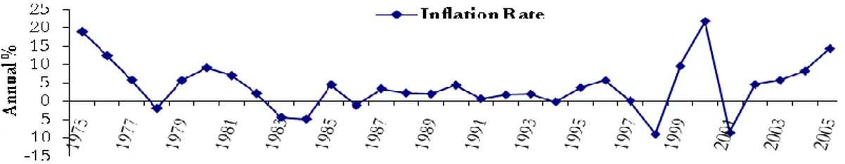
The large boost in U.A.E‟s development and economy is founded on the export of the country‟s oil and petroleum-based products since 1958, when oil was first discovered in Abu Dhabi (Sharply, 2002). Almost 10 percent (%) of the world‟s current oil reserves are controlled by the U.A.E, enabling it to command more than 16% of OPEC‟s total reserves (Davidson, 2007). According to OPEC (2007), crude oil production in U.A.E during 2007 reached a daily average of 2.5 million barrels per day. Even though there is a nominal exis-tence of a federal Ministry of Oil and Petroleum Resources, U.A.E‟s oil policy remains to exist under the operation of the emirate-level governments (Davidson, 2007). One of the threats towards U.A.E‟s economy is considered to be a high inflation rate, which is on par with the world‟s highest (Schwab & Porter, 2008-2009). It reached 14.3% in 2005 as listed in the World Development Indicators (WDI) database, 2008. There are several factors con-tributing to the increasing prices; the high rate of economic growth, increasing oil prices and the increasing demand in the country due to investment projects in the infrastructure. Furthermore, the situation of U.A.E‟s currency, the dirham (AED), is pegged at 3.6725 to the U.S. dollar (USD) according to the International Monetary Fund (IMF, 2008). The pegged currency contributes strongly to the inflationary problem, making it more difficult to control fluctuations in the economy. Figure 1 below illustrates the fluctuation in the in-flation rate from 1975-2005. As can be seen in the figure the U.A.E has experienced peaks in 1975, 1980, 2000 and 2005 and lows can be seen in 1978, 1984, 1998 and 2001.

Figure 1: Changes in Inflation from 1975-2005

Source: Nation Master‟s Economy Statistics, 2008

1 _{The authors would like to highlight that U.A.E still consists of deserts.} 2 _{Current prices}

A discussed topic of U.A.E‟s economy is their aim to minimize its dependency on oil; therefore much focus has been targeted on diversifying the economy during the past two decades. In turn, making it more dependent on the service sector: especially high-class tourism as well as expanding the international finance sector. In both developed and devel-oping countries, a natural resource boom, (as experienced in U.A.E) has triggered the so called „Dutch Disease‟. A theory that originates from the Netherlands in the 1970s, basi-cally explaining a decline in the traditional manufacturing sector when the country experi-ences a boom in their natural resource. The Dutch Disease indicates that the natural re-source abundant factor, (natural oil in U.A.E‟s case), triggers an appreciation of the domes-tic currency. In a pegged-currency economy on the other hand, the inflation rate increases. A result of the increasing export sales and the rising “real” exchange rate (RER). In turn, other non-resource exporters are affected at the same time and the manufacturing sector experiences a constrained activity to compete in the world market. Furthermore, the agri-cultural sector undergoes a decline as labour moves to either the booming sector or the non-tradable sector (Sachs & Larrain, 1993). The case of the Dutch Disease would be a problem to the U.A.E since it causes the shift of labour and production for the tradable sector to the non-tradable sector causing a decline in the country‟s exports of manufactur-ing and agricultural goods.. The decline in exports of U.A.E‟s traditional tradable goods de-creases production of the goods affecting the country‟s economy in a negative way. Fur-thermore, since U.A.E is faced by a high inflation rate the possibility of the Dutch Disease could increase the inflation rate even more, putting further constrains on the economy in how to deal with the existing inflationary problem.

1.1

Purpose

The purpose of this paper is to study U.A.E‟s development in economic growth since 1975 until 2005 and establish if there are any signs of the Dutch Disease by testing the ratio of tradable goods to non-tradable goods and the effects by other macroeconomic variables. Therefore the authors of the thesis apply the following research question.

 Did the oil boom in the U.A.E during the 1970s lead to symptoms of the Dutch Disease throughout the period 1975-2005 and if so, to what extent?

1.2 Outline

The authors have focused on giving the readers an introduction to the topic in hand and purpose for the first section in this thesis. As the readers may not be familiar with the cho-sen country, the authors precho-sent a brief history of the economy followed by previous stu-dies in the second section. Section three contains a relevant definition, applicable theories illustrated with graphs as well as a summary of the applied theoretical models and following this are the hypotheses. The next section presents the data for the macroeconomic va-riables implemented, descriptive statistics with analysis, followed by an earlier empirical model and adapted regression models applied for the authors‟ purpose. Furthermore, eco-nometric problems and the OLS test results and analysis are also presented in section four. Finally, the authors provide conclusions of the thesis in section five as well as suggestions for further research.

2 U.A.E Background and Previous Studies

U.A.E consists of the seven emirates Abu Dhabi, Dubai, Sharjah, Ra´s al-Khaimah, Ajman, Umm al-Qaiwain and Fujairah, which are located on the southern Arabian Gulf. On the 2nd of December 1971, the country became independent after being under British rule for a period of 70 years. The independence and discovery of oil triggered the economic devel-opment in U.A.E which led to a huge expansion in the population. In 2007 the population reached 4.36 million as listed in the World Bank, 2008. Five decades earlier there were only a few hundred thousand inhabitants (Davidson, 2007).The population boom in U.A.E is a result of the increased demand for labour throughout the past four decades and consists for the most part (83%) of labour from foreign countries referred to as expatriates (David-son, 2007). According to the International Labour Organization (ILO, 2008) total em-ployment in 2005 reached 2.47 million compared to a low total unemem-ployment of 0.79 mil-lion. Furthermore, United Nation‟s (UN) database illustrates the division of the labour from two perspectives; first from the year 2000 compared to the changes that prevailed in 2006. Female participation and male participation in 2000 consisted of 34.4% in the former group and 92% in the latter group.

As stated in the introduction, one of the impacts when an economy is experiencing signs of the Dutch Disease is the high inflation rate followed by a change in the real exchange rate. Fluctuations in the real exchange rate can cause resources and production to reallocate be-tween the economy‟s sectors‟ of tradable and non-tradable goods and services and is there-fore regarded as an important price in the economy according to Karam (2001).

The U.A.E is one of the countries in the Middle East which follows a pegged (or fixed) ex-change rate regime, in which foreign central banks stand ready to buy and sell their curren-cies at a fixed price in terms of dollars (Dornbush, Fisher & Startz, 2008). The currency of the U.A.E, the AED was first officially pegged against the USD in 1974. By the end of 1977 fluctuations occurred widely. One year later it became pegged to the Special Drawing Right3_{, (SDR), whilst the USD remained as the intervention currency with the initial selling}

rate of 3.88 AED to 1 USD. Since November 1980, the currency has been hard pegged to the USD at 3.67275 AED for 1 USD. For over two decades the USD had been used as an anchor currency in practice when it became the official anchor currency in 2002. The deci-sion to make the USD an anchor curreny was made by the member nations of the Gulf Cooperation Council (GCC) in order to establish a common currency in 2010 (Schuler 2004).

The U.A.E and the effects from the oil industry has not been studied to any great extent. However some studies on the Dutch Disease concerning other countries have been conducted, but these studies are mainly theoretical and lack econometric testing. The studies with statistical analysis contain time series, more observations and flexible exchange rates (which could be included in the regression model). In order to make it more comprehensive and easier for the reader, the previous studies on similar topics is listed in table 2 below.

3 _{SDR was originally created in 1969 by the IMF in order to support the Bretton Woods fixed exchange rate}

system. Today, SDR‟s function is to serve as IMF‟s unit of account as well as for other international organiza-tions (IMF, 2008).

Table 2: Previous Studies Condu cted on Similar Topics

Earlier Literature Key Findings

H. Falck

(1992) Dutch Disease shows that it is possible for foreign aid to give rise to an appreciation of the RER, causing deteriorating effect on the international sectors in Tanzania. Discusses alternatives which may cure the disease. K. Miagra,

O De Silva (1994)

Stresses the importance of government policies during a resource boom by using the Dutch Disease as a case study of several countries, e.g. Nigeria and Mexico. Highlights that recent developments in trade theory has to some degree “justified” government policies which would have been predicted as “irrational” according to standard eco-nomic theory. Fiscal, monetary and exchange rate policies assumes to maintain the domestic demand by interaction by governments.

H. Imai (2000)

N. Oomes, & K. Kalcheva (2007)

Discusses if Hong Kong‟s high inflation was due to The Balassa-Samuelsson Effect or the Dutch Disease. A case of a fixed currency. Results show that the Dutch Disease was the main reason for the long-term rate of inflation.

Even though a country (Russia in this case) may have all the symp-toms it still may be difficult to diagnose if the economy is suffering from the disease. Symptoms of the disease can be explained by other factors. Rising levels of remittances and spending effects lead to the disease.

3 Theoretical Framework

In order to comprehend the Dutch Disease theory the authors used Sachs and Larrain‟s (1993) theoretical model of tradable (T) and non-tradable goods4 _{(NT), also known as the}

TNT Model. The model is a simple theoretical model which describes the diversification of goods from tradables to non-tradables.

3.1 The TNT Model

According to Sachs and Larrain (1993) the most important assumptions is that N can nei-ther be exported nor imported and its domestic consumption and production must be equivalent. The opposite applies for T, consumption and production domestically can dif-fer because of the possibility of imports and exports T. In this specific model, two goods are produced and consumed: T and N by one factor of productivity which is labour. The supply side obtains two linear functions:

QT = aTLT (T) and QN = aNLN (N),

where production is dependent on labour. LT and LN accounts for the amount of labour

used, whilst aT and aN are the marginal productivities of labour for the two sectors. In other

words aT or aN units more of output is achieved if one extra unit of labour is applied in

ei-ther sector. Due to the linear functions, aT and aN also account for average productivities.

The demand side of the TNT model circles around consumption decisions which do not include investment spending. Total absorption, i.e. spending on T and N is expressed in the equation as followed:

A = PTCT + PNCN.

Total absorption is defined by A and levels of consumption for T and N by CT and CN. PT

and PN corresponds to the price of the goods. Furthermore, Sachs and Larrain (1993)

as-sume if the ratio CT/CN is fixed, then households consume CT and CN in fixed proportions,

(regardless of relative prices). If overall spending increases, it is followed by an increase in consumption in T and N by the same proportion and vice versa.

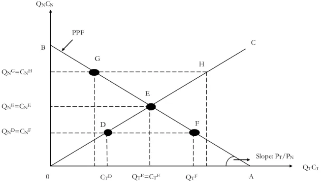
Figure 3.1 below illustrates the production possibility frontier (PPF), the consumption line and the market equilibrium for T and N in a country. The PPF shows each quantity of QT

that is produced in order to produce the maximum quantity of QN. If QN = aNL then QT =

0, represented by point B in the figure. Then the factor of productivity labour is located in the N sector. If QN = 0 and QT = aTL, then labour is located in T (point D in the figure).

The slope of the PPF is equal to PT/PN, i.e. the relative price of T in terms of N, which is

also referred to as the real exchange rate, „e‟, in the TNT model. Therefore, aN/aT = PT/PN

= e.

The production of a unit of a good either in T or N and the labour cost used is equivalent to the output price. The consumption line is represented by the 0C line in the figure. When absorption (A in the equation above) is low then households spend an amount equal to point D and when absorption is high household spending is equal to H. At point D, CT and

CN are both low and at point H, CT and CN are high. The ratio CT/CN is fixed as absorption

4 _{A tradable goods and non-tradable good is defined according to the standard industrial classification (SIC),}

developed by the UN. In general a tradable good is produced in agri culture, mining, quarrying or manufac-turing and can be traded, a non-tradable good can not be traded su ch as services within retail trade, hotels, restaurants, businesses, financing and real estate.

increases or decreases along the 0C line. Point D represents household consumption, where CD

N and CDT consist of the consumptions of N and T respectively. Indicating that

production of N must also equal to CD

N5, hence QFN = CDN. Therefore the production

point has to be on the PPF at the same point where QN = CN, i.e. point F. The production

point for absorption and point D, household consumptions rests on the identical horizon-tal line. The economy is faced by a trade surplus when production of T is located on point F and point D accounts for absorption since QF

T > CDT , (i.e. production is larger than

ab-sorption). One conclusion is drawn by the comparison of the points H and D: spending in-creases on both goods when absorption in general is high. The balance between demand and supply for N holds when a pressure on demand for N is met by increased production within the same sector. This takes place if resources are shifted out from the T sector and placed into the N sector. Facing an increase in demand, the economy will experience a de-crease in production of T as production of N on the other hand will inde-crease. Equilibrium in the economy occurs at point E, i.e. consumption and production for both goods are equivalent leading to a balance of the trade account where CT = QT.

3.2 The Dutch Disease Models

In the case of fluctuations in the level of domestic spending, one possible effect is that production shifts between sectors: from tradables to non-tradables. The scenario occurs when a country faces a significant change in wealth due to a new discovery of a resource or when there are shifts in the price of resources. During the 1960s, the Netherlands expe-rienced a discovery of natural gas leading to exports of the resource to rise dramatically which caused the currency, the guilder to appreciate. This resulted in a decline in the wealth of other exports such as manufactures (Sachs & Larrain, 1993), hence the name, the Dutch Disease. The authors have applied the Corden and Neary‟s (1982) core model, Corden‟s

5 _{Since consumption must equal produ ction in N.}

B C H QTCT A F E G D QNCN 0 CTD QTE=CTE QTF QNG=CNH QNE=CNE QND=CNF

Source: Sachs & Larrain, 1993, p.664

Figure 3.1: The PPF, the Consumption Path & Equilibrium

Slope: PT/PN

(1984) extended core model and Sachs and Larrain‟s (1993) Dutch Disease theory which are presented below.

3.3 The Corden and Neary Core Model

The Corden and Neary Core Model (1982) is a further development of the Salter non-tradable model referred to as the basic framework for the Dutch Disease from 1959. In which an economy produces three types of goods: two traded and one non-traded. The ex-tended core model from 1982 established two effects related to the de-industrialisation of the traditional manufacturing sector, more known as the spending effect and the resource movement effect (Corden & Neary, 1982). Corden presented the core model again in 1984, which consists of three sectors in a small economy; the booming sector (B) and the lagging sector (L) produce the tradable goods (T). The former sector could include oil, gas or a mineral industry and the latter a manufacturing industry. The final sector non-tradable sec-tor (N) produces the non-tradable goods such as services. Furthermore, capital, a secsec-tor specific factor and labour, the common factor of production are both used in the three sec-tors.

If sector B would experience a boom, then it is considered to happen in one of three ways according to Corden (1984); (1) Sector B faces exogenous improvements within technolo-gies, (2) Supply in the specific factor increases due to a recent detection of resources or (3) B produces only for exports with no sales in the domestic country and there is an increase in the world market prices compared to import prices. Corden and Neary (1982) focused on example 1.

3.3.1 The Spending Effect

One of the effects developed in the 1982 core model was the spending effect, which occurs when disposable income rises due to a boom in B and an inflow of foreign exchange. The additional income is spent by the employer directly or indirectly by the government through extra tax revenue. The inflow is either invested in imports (which has no direct impact on the demand for goods domestically produced) or in the money supply within the country. On the other hand, the foreign exchange can be converted into the local currency and later be invested in the N sector‟s goods. Income elasticity for N assumes to be posi-tive causing demand and spending for N and T goods to increase. The price of T does not increase at all or nearly as much as N since world demand is not affected by the increased domestic demand in the assumed small economy. Furthermore, the price increase leads to two possible outcomes; (1) The real exchange rate appreciates therefore the world market for T becomes less competitive and (2) Wages within the sector for N rises, resulting in a shift of labour to the N sector from T, which proceeds until factor prices amongst the three sectors becomes equal.

In the case of a fixed exchange rate, the country‟s money supply would rise if the foreign currency is converted into the local currency. Furthermore prices on domestic goods in-creases as a result of a push in domestic demand. The “real” exchange rate appreciates, i.e. “real” goods and services in the domestic economy become more expensive and a unit of the foreign currency buys fewer goods than previously. The appreciation in turn affects the exports for the country, which becomes less competitive, therefore leading to the two poss-ible outcomes mentioned above (zadeh-Ebrahim, 2003).

3.3.2 The Resource Movement Effect

The other outcome from the Corden and Neary (1982) Dutch Disease core model is the resource movement effect which is split into two effects: direct and indirect resource movement effect. The former has an outcome also known as direct de-industrialisation ex-plained as followed; in addition to the boom in B, the marginal product of labour rises causing wages to go up. This puts a pressure on the demand for labour in B. Labour in L and N continues to shift towards B until wages are equalized in the sectors. The shift in la-bour occurs without impact on the real exchange rate thus the N market and its lala-bour is unaffected. The latter effect is due to the cutback in production in N, a result of unchanged demand. Excess demand occurs because of the reduced supply, making prices rise followed by a wage increase in N thereby, labour in L continues to shift towards N.

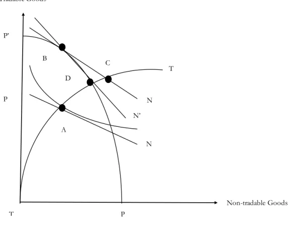
Illustrated in the figures below (3.3.2 and 3.3.3) are the two effects, the spending effect and the resource movement effect, presented by Falck in 1992. The sectors B and L are com-bined into one entire sector, where price is determined by the world market and is norma-lised to one. The domestic market however determines the price of N, i.e. PN, which helps

trigger the equilibrium in the economy. The output of N and T are measured on each axis in the graph, N by the X-axis and T by the Y-axis. Point A in the graph illustrates the initial equilibrium in the economy which is defined as equality between supply (XN) and demand

(CN), i.e.

XN(PN) = CN(PN,Y).

Variable Y represents income and is equal to the production value of T and N plus F, the capital inflow, i.e.

Y = PNXN + XT + F.

The production possibility (PP) curve, i.e., the PP line in the graph shows the economy‟s total amount of goods available. Furthermore, point A lies on the slope of PP curve which is tangent to the attainable slope of the social indifference curve which lies furthest out from the origo. The tangible location also determines the price of N. The TT curve corres-ponds to the income-consumption curve. When a boom occurs in the economy, the avail-able amount of goods increase leading to that the PP curve shifts outwards to the PP‟ curve. The shift leads to additional output in T but unchanged output for N.

Falck (1992) assumes that the resource movement vanishes if capital inflows are invested so that the common factor of production is used, which gives way to the upward shift of the PP triggered by a boom. Point B that is vertically above the initial production point A represents the new production point if the price of N remains the same as before. The in-come-consumption curve, i.e., the TT curve intersects with the price line at point C, which illustrates the bundle of goods demanded at the current price. Consequently, excess de-mand of N corresponds to the distance between B and C. In order to stabilize the market the price of N must increase. As a result, production within sector N will begin to increase and pressure on demand will decline. The new equilibrium will be located on the PP‟ curve, someplace between the intersection of the PP‟ curve and TT line, for instance at point D. The spending effect therefore concludes that production in the T sector has decreased and vice versa in N, which has increased.

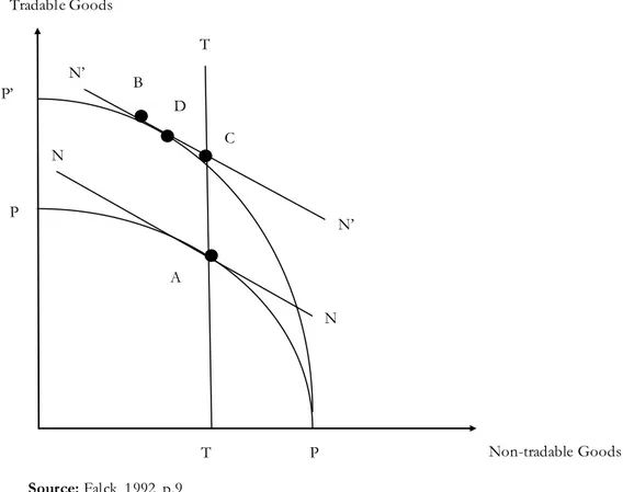
In order to single out the resource movement effect (see figure 3.3.3), Falck (1992) assumes that N‟s income-elasticity is equal to zero and the spending effect is therefore eliminated. As illustrated in the figure the TT line (income-consumption line) vertically goes through point A. In the case of a boom and PN remaining unchanged, the new production point is

located at point B. As a consequence, marginal productivity of labour and wages increase. The changes in wages make a shift of the common factor of production from L and N to-wards the B sector. Accordingly an increase occurs in B as well as the combined T sector, while N experiences a decrease. Point C is where the bundle of goods demanded is located when PN remains unchanged, i.e. on the intersection on the TT line and NN line. An

excess of demand for T occurs like in the spending effect. In order to reach an equilibrium in the market, prices of N need to rise, consequently the final equilibrium will be at point D, someplace between the intersection of the PP‟ line and the vertical TT line. The re-source movement effect causes production in N to decline while T rises. Falck (1992) high-lights two specific moves in the diagram which represents the case of direct resource movement effect and the indirect effect. The shift from A to B corresponds to the former and the last mentioned is the shift from point B to point D.

P P P‟ N‟ N N T C D A B Non-tradable Goods Source: Falck, 1992, p.7 T

Figure 3.3.2: The Spending Effect

3.4 Dutch Disease - Sachs and Larrain

Sachs and Larrain (1993) stress that the consequence of discovering a natural resource such as oil is the decline in production in the traditional manufacturing sector, causing the sector to shrink. Thereby workers and owners in the specified sector are affected more negatively by the disease. However, there is also a positive effect of the boom in natural resources, i.e., the resources can be drawn away from the traditional T sector and into the N sector in-stead.

The figure below (3.4) illustrates possible effects if a natural resource such as oil is discov-ered in the country. Prior to the discovery, T was dominated by non-oil industries, e.g. manufacturing. The line PF is the PPF before the boom. Q0 shows the increase in T due to

the booming sector, i.e. Q0 more units of T were produced. Resulting in a shift (equal to

the amount of Q0) in the PPF towards the right, as can be seen in the figure. Point A is the

initial economic equilibrium which shifts to point B due to the boom. As a result of the boom, demand increases causing a rise in consumption of both N and T, the spending boom is shown in the increased production of N, which shifts from QA

N to Q B

N.

The increased production of T is illustrated at point B, where the production of non-oil tradables is at level QB

T and the oil production is at Q0; i.e. the total T production is at the

level QB

T+Q0. When comparing the change in production in T prior to and after the

dis-covery of the natural resource, three conclusions can be made which are referred to in the diagram as 1, 2 and 3. (1) Non-oil production decreases from QA

T down to Q B

T, (2)

Pro-duction of oil increases from zero to Q0 and (3) The sum of the two sub sectors, i.e. total

trade production increases from QA

T to QBT+Q0. Figure 3.3.3: Resource Movement Effect

T Tradable Goods N‟ N‟ N N T Non-tradable Goods P P B D C A P‟ Source: Falck, 1992, p.9

Figure 3.4: Effects of Oil Discovery in a Hypothetical Country: A Case of Dutch Disease

Source: Sachs & Larrain, 1993 p.669

In order to make the models more comprehensive for the reader, the authors summarized them in a table 3.4 below, pointing out the most relevant key findings.

Table 3.4: Summary of Models

Type of Model Key Findings

The TNT Model: Sachs and Larrain (1993)

- Overall spending increases on both goods, T and N when absorption in general is high and vice versa.

- Demand and supply for N is balanced when a rise in demand for N is met by increased production within the same sector, which occurs if resources shift out from the T sector and into the N sector.

- Facing an increase in overall demand, the economy experiences a decrease in production of T as production of N on the other hand will increase. - An increase in demand for N only is satisfied by further production domestically whilst if demand for T increases it is met by imports.

The DD Model: Corden and Neary (1982)

- The economy consists of 3 sectors: the booming sector (B) and the lagging sector (L) produces the tradable goods (T) and the non-tradable sector (N) produces the non-tradable goods such as services.

- A boom occurs in one of three ways: the core model concentrates on exam-ple (1) which is due to exogenous improvements within technologies in sector B.

- The spending effect occurs when the economy faces a rise in disposable

in-come, due to a boom in B and and an inflow of foreign exchange.

A QN QT C 0 QA QB QTB QTA QTB + Q0 P B 1 3 Q0 2

- The demand for N increases causing the relative price of N to T to become higher. The price of T may increase but not as much as the change in T. - The change in price leads to (1) Appreciation of the real exchange rate, in turn competitiveness for T in the world market declines and (2) Wages within the sector for N rises, resulting in a shift of labour to the N sector from T. - The resource movement effect can either be the direct or indirect, the for-mer is also referred to as direct de-industrialization. Direct resource move-ment effect occurs when the marginal product of labour and a boom in B rises simultaneously causing wages to increase. Labour in L and N shift to B until wages are equalized. In the indirect resource movement effect, excess demand occurs due to reduced supply, prices and wages increase in N, caus-ing labour in L to shift to N.

The DD Model – Sachs and Larrain (1993)

- The disease causes a negative and positive effect: The former is the decline in the traditional manufacturing sector and latter is that resources can be drawn away from T and into N instead.

- Three conclusions are made when comparing the change in production in T in the model and after the boom; (1) Non-oil production decreases, (2) Pro-duction of oil has increases from zero and (3) The sum of the two sub sec-tors, i.e. total trade production increases.

3.5 Hypotheses

Based on the background and the theoretical framework it is possible to ask if the oil boom in the U.A.E during the 1970s lead to symptoms of the Dutch Disease throughout the time period 1975-2005 and if so, to what extent?

According to this question, the following hypotheses are stated as followed:

Hypothesis 1: The price of oil (P) during a boom in natural resources has a negative (or

no) effect on the ratio of tradable goods to non-tradable goods.

The reasoning behind this hypothesis is because the world market determines the price of the tradable goods causing an appreciation of the “real” exchange rate. Prices in tradables may not increase at all or not as much as non-tradables. Since prices in the non-tradable sector increases due to an excess demand because of limited resources, production of the sector rises in compared to the tradable sector, hence labour shifts from tradables to non-tradables.

Hypothesis 2: During a boom in natural resources, inflation (I) has a negative effect on

the ratio of tradable goods to non-tradable goods.

The statement is based on the presented theory that during a boom period in a country with a fixed exchange rate, an inflow of foreign exchange increases the money supply if converted into the local currency. In turn, the “real” exchange rate appreciates, making the domestic goods and services more expensive. Exports of the country become less competi-tive and wages within non-tradable sector rise resulting in a shift of labour from the trad-able sector to the non-tradtrad-able sector.

Hypothesis 3: The Dummy variable (D1) has a negative (or no) effect on the ratio of

tradable goods to non-tradable goods.

The final hypothesis is dependent on the high oil prices U.A.E experienced during the pe-riod 1975-1980. Therefore the reasoning is equivalent to hypothesis 1.

3.6 Method and Limitations

In order to perform the regressions in this thesis the authors test two different models with different sets of variables. The analyses are based on time series estimations with annual da-ta from 1975 to 2005, i.e. 30 samples and the method used is the Ordinary Least Squares (OLS). The data for the period tested are collected from various databases, primarily from UN (2008) and U.A.E Ministry of Economy (2008). All the data collected is in AED except the price of oil, which is in USD per barrel. The ratio of tradable goods to non-tradable goods is calculated by the authors. The sum of the data for manufacturing and agriculture (tradable goods) is divided by the sum of services (non-tradable goods). The oil revenue is not included in tradable goods, since the purpose of the regressions is to see if the non-oil sectors i.e. manufacturing and agriculture have increased or decreased as a result of the oil boom in U.A.E. The variables tested in this thesis are; ratio of tradable goods to non-tradable goods (R), inflation (I), price of oil (P) and in the second regression one dummy variable (D1) is added. D1 represent the years 1975-1980. The reason why this specific time period is selected for D1 is due to the changes in the price of oil during these years.

4 Empirical Findings and Analysis

4.1 Data

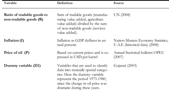
In order to make it more comprehensive for the reader, the authors made a summary of the collected data, i.e. an explanation of the macroeconomic variables in table 4.1 below, giving a definition of the data and where it was retrieved from.

Table 4.1: Summary of the Macroeconomic Variables used in the Regression

Variable Definition Source

Ratio of tradable goods to

non-tradable goods (R) Sum of tradable goods (manufac-turing value added, agriculture

value added) divided by the sum of non-tradable goods (services value added).

UN (2008)

Inflation (I) Price of oil (P)

Inflation as GDP deflator in an-nual percent.

Based on current prices and is ex-pressed in USD per barrel

Nation Masters Economy Statistics, U.A.E (historical data) (2008) Annual Statistical bulletin OPEC (2007)

Dummy variable (D1) Variables that are used to classify

data into mutually special catego-ries. Here the dummy variable represent the period 1975-1980, since the change in oil price was dramatic during these years.

Gujarati (2003)

Other variables were also tested, but due to insignificant values and to avoid problems of correlation, some of the variables were excluded from the regression models. One of the other variables tested was money supply (M1), but since this variable was highly correlated with GDP, the authors decided to exclude it. GDP was also excluded due to high correla-tion with the price of oil. Two other dummy variables for the periods 1980-1985 and 2000-2005 were tested, but since they were not significant, they were also excluded from the re-gression model.

4.2 Descriptive Statistics

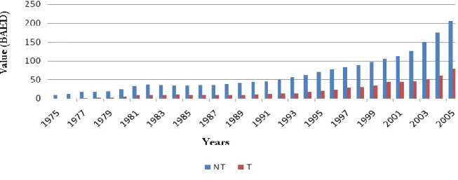
The following figure shows the change in value added of tradable goods6 _{and non-tradable}

goods in U.A.E throughout the period 1975-2005 expressed in billion of AED per year.

Figure 4.2: Value Added in Tradables and Non-tradables in U.A.E, 1975-2005

Source: UN, 2008

As can be seen in figure 4.2, the production of non-tradable goods has been larger than tradable goods (non-oil goods) during the entire period. The tradable sector has not in-creased as much as the non-tradable sector, i.e. non-oil production has dein-creased in com-parison to non-tradables, supporting conclusion 1 of Sachs and Larrain (1993). In fact the non-tradable sector has increased almost twice as much as the tradable sector, which is a symptom of the Dutch Disease. One of the reasons why the non-tradable sector may have increased so much could be due to the country‟s rise in export of oil throughout 1975-2005. The income from the increased exports is converted into the local currency and may be used to finance the non-tradable sector. Thereby production of non-tradable goods in-crease which is in line with the spending effect presented by Corden and Neary (1982). The figure below displays the value added in the three sectors, expressed in billions of AED per year.

Figure 4.2.1: Value Added in Agriculture, Manufacturing and Services in U.A.E, 1975-2005

Source: UN, 2008

Figure 4.2.1 illustrates a clearer distinction of how production in the three sectors has changed during the 30 years. It is clear to see that the service sector holds a stronger value added compared to the non-oil sectors and has had a sharp increase since 1993. It can be seen in figure 1 in the appendix that the U.A.E‟s oil production reached a peak in 1992.

The high level of production continued but experienced a fluctuation between the years 1998-2003. The authors can therefore highlight that during the 1990s oil production in-creased possibly due to the low oil prices which existed during the same time (see figure 4.2.2). The overall increase in oil production is a symptom of the disease according to Sachs and Larrain‟s (1993) second conclusion that production of oil increases.The fact that there was no cutback in production in the non-tradable sector rules out possible assump-tions of the indirect resource movement effect. Furthermore, the situation of a high pro-duction of non-tradables, high oil propro-duction but a low value added of manufacturing and agriculture7 _{is consistent with the first outcome of the spending effect.}

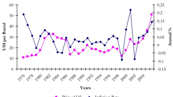
Figure 4.2.2 illustrates the relationship between the price of oil and the inflation rate during the period 1975-2005. The authors will concentrate on analysing the inflation rate‟s peak and lows and the impact from the fluctuating oil price.

Figure 4.2.2: The Inflation Rate and the Price of Oil in U.A.E, 1975-2005 The Price of Oil and Inflation Rate

0 10 20 30 40 50 60 1976 1978 1980 1982 1984 1986 1988 1990 1992 1994 1996 1998 2000 2002 2004 Years U S$ p er B ar re l -0.15 -0.1 -0.05 0 0.05 0.1 0.15 0.2 0.25 A nn ua l %

Price of Oil Inflation Rate

Source: Nation Master‟s Economy Statistics, 2007

The authors can first see that there was a sharp decline in inflation from 19758 _{until 1978.}

During 1974 the inflation rate was 138.26% according to Nation Master Economy Statis-tics (2008). The sharp decline could be due to that the U.A.E officially pegged the AED to the USD in 1974. The fluctuation in the inflation rate cannot only be explained by a boom in production but also depends on other factors as well, such as the depreciation of the USD. Due to U.A.E‟s pegged currency to the USD, the country experiences inflationary problems as the dollar depreciates (Arnerich et al, 2007).

During the period 1978-1980 the price of oil and the inflation rate increased at a steady rate, a possible result of the oil price shock that took place in 1979 which had a negative impact on the inflation rate. In 1998, the inflation rate and the price of oil were almost at the same point in the figure followed by a sharp increase in inflation and a steady rise in the

7 _{Tradables have increased slightly during the years however the increase in production has not been enough}

to consider that the tradable sector has a high value added su ch as the non-tradable sector.

price of oil, which reached a peak in 2000. The inflation rate then plummeted down to-wards an almost equivalent negative value as in 1998. One of the reasons why the inflation in U.A.E change so dramatically during the years 1998-2001 could be due to the burst of the “I.T-bubble” (know as the “Dot-com bubble”) in the late 1990s which affected USD negatively.

Furthermore, there can also be some political explanations to the high inflation problem in U.A.E. The problem could be due to the split population consisting of expatriates and na-tives affecting the U.A.E government and economy. Expatriates are imported to the coun-try in order to solve the problem of the lack of labour supply of the native population. However, expatriates might decide to leave the economy due to the living standards and low wages. In order to overcome this problem foreign countries sign protocols to protect their citizens from these poor working and living conditions. This will in turn increase companies‟ costs, which leads to a higher inflation rate within U.A.E (Foley, 1999).

4.3 An Earlier Empirical Model

The authors are inspired by Lartey, Mandelman & Acosta‟s (2008) study „Remittances, Ex-change Rate Regimes, and the Dutch Disease: A Panel Data Analysis‟, in which the rela-tionship between remittances and other macroeconomic factors are tested in order to find any presence of the Dutch Disease in 109 developing and transition countries for the pe-riod 1990-2003. The macroeconomic variables used in their study are: GDP, money supply (M2), trade index (goods and services), trade openness (sum of exports and imports as a percent age of GDP) and GDP growth (in percent). The model implemented was a dy-namic panel data model, estimated by using generalized method of moments estimator (GMM), which was adapted to deal with endogeneity in the explanatory variables. Two dif-ferent equations were used to determine possible signs of Dutch Disease on remittances in the countries chosen. The dependent variable for the first equation is the ratio of tradable to non-tradable output (used to determine the resource movement effect) and the second equation has the real exchange rate as the dependent variable. Lartey, Mandelman & Acosta (2008) wanted to test if the spending effect and the resource movement effect of remit-tances were different under alternative exchange rate regimes. The tradable output is the sum of manufacturing and agriculture and the non-tradable output is the sum of services.

The Model:

yit= ∑pj=0 αj ri, t-j + βxit + (ηi + λt + εit) i= 1,2…N t= 2,3…T

In the model above the variable yit is the dependent variable for country, i, in period t. In

the first regression model y stands for the ratio of tradable to non-tradable output and in the second model for the real exchange rate. Variable rit is remittances and is assumed to be

endogenous and p is the lag length to find the postponed effects of remittances on the productive sectorial structure. The variable xit is a vector of current values of additional

ex-planatory variables and it is assumed to be endogenous. ηi is a variable that stands for the

stochastic unobserved country-specific time-invariant effect. λt is included to account for

time-specific effects. ε is the disturbance term and is assumed to be serially uncorrelated and independent across individuals.

Lartey, Mandelman & Acosta (2008) found that an increase in remittances results in a de-crease in the shares of agriculture and manufacturing in GDP. Moreover, the share of ser-vices in GDP increases when remittances increases. Further results show that when GDP

per capita rises, the share of services increases, the share of agriculture on the other hand decreases. Furthermore, countries with a fixed exchange rate experience a larger real a p-preciation leading to a rise in remittances. The sign of Dutch Disease in their test is that the share of services in total output increases whilst the share of manufacturing decreases and that the effects of the disease is stronger in countries with fixed exchange rate regimes than in countries with a flexible exchange rate. According to the results, only countries that have a nominal exchange rate peg experienced a resource movement effect in favor for the non-tradable sector.

4.4 The Regression Model

In order to test if the chosen macroeconomic variables show indications of symptoms of the Dutch Disease, the model with the ratio of tradables goods to non-tradable goods from Lartey, Mandelman & Acosta (2008) was adopted but adjusted in order to fit this thesis. The adjusted equation is based on time series data. The presented macroeconomic vari-ables; inflation (I) is based on the theoretical framework presented, price of oil (P) is adopted from Oomes & Kalcheva (2007), which included price of oil in the regression analysis. The dummy variable (D1) for the period 1975-1980 is inspired from Vos (1998) which included a dummy variable for a one year period. Furthermore the authors used the OLS method. The real exchange rate is replaced by the inflation rate, since the fixed ex-change rate in U.A.E is unaffected by symptoms of the disease. A variable consisting of the high inflation rate on the other hand could serve as a sign for the Dutch Disease problem. The ratio of tradable goods to non-tradable goods serves as the dependent variable in both models, however the independent variables differ slightly; the first regression model in-cludes inflation and price of oil as the independent variables. The second regression model also includes inflation and price of oil but a dummy variable for the period 1975-1980 was added. Model 1: R = β0 + β1P + β2I + ε Model 2: R = β0 + β1P + β2I + β3D1 + ε 4.4.1 Econometric Problems

In the beginning of the regression testing the authors discovered that some of the variables were correlated with one another. Money supply (M1) and GDP were the most correlated variables in the regression models, so in order to avoid multicollinearity problems the a u-thors decided to exclude money supply and GDP from the regression model. The reason why the two variables were excluded, was due to the high correlation between GDP and money supply and the high correlation between GDP and price of oil. Another problem the authors found was insignificant values when testing the regression models with dummy variables. From the beginning three dummy variables were included, for the periods 1975-1980 (D1), 1975-1980-1985 (D2) and 2000-2005 (D3), but since D2 and D3 were insignificant the authors decided to exclude them from the second regression model, since they did not contribute to the regression resul. Another regression with annual change over the years in each variable was also performed, but the results from that regression were not significant, so the authors decided to leave out that regression as well.

4.4.2 Expected Signs of the Variables

Based on the theories presented in the theoretical framework the authors decided the pat-terns of the variables as listed in table 4.4.2 below.

Table 4.4.2: Expected Signs of the Variables Tested

Coefficient Sign

β1 (Price of Oil) negative or no effect

β2 (Inflation)

negative

β3 (Dummy Variable) negative or no effect

4.5 Regression Results

In order to make it more comprehensive for the reader, the authors summarized the coef-ficients and significance levels (1%, 5% or 10%) from the two different regression model results with 31 observations for the period 1975 to 2005 in table 4.5 below. The probability value (p-value) is used instead of fixing the significance level at a specific level since the probability value is known as the exact or observed significance level.

As can be seen in table 4.5, the goodness of fit for the models is relatively strong. The R-square values show that 39.3% (model 1) and 75.3% (model 2) of the change in the ratio of tradable goods to non-tradable goods can be explained by the model used. The goodness of fit in model 1 on the other hand, has a poorer fit, where 39.3% of the influences on the dependent variable can be explained by the model. The better fit of model 2 can be due to the additional variable tested in the second regression model, i.e. D1. Furthermore, the Durbin-Watson values indicate that positive serial correlation may be present in the regres-sion models, in model 1 where it is equal to 0.238252 and model 2 (0.416614). By address-ing to the correlation matrix, the explanatory variables implemented in the two models in-dicate that one of the variables tested are highly correlated with the dependent variable. This variable is D1(-0.817021, see appendix table 4) indicating a sign of collinearity prob-lems in the second model. The first regression model shows no signs of any multicollineari-ty problem, since none of the variables are highly correlated with another variable (appen-dix table 2).

In model 1 and 2 the price of oil is significant and does not support the expectation that it would have a negative or no effect on the ratio. Price of oil is significant at a 1% signific-ance level in model 1 and affects the dependent variable positively. A 1% increase in the ra-tio of tradable goods to non-tradable goods would increase the price of oil by 0.005840%, all else equal. In the second regression model, the price of oil is significant at a 1% level, meaning that a 1% change in the regressand would increase the price of oil by 0.002988%, all else equal.The results from the regression models indicate that the price of oil has a pos-itive effect on the dependent variable. According to the spending effect from Corden and Neary‟s (1982) core model a boom in the booming sector is followed by an inflow of

for-eign exchange which can be converted into the local currency. The converted inflow causes the money supply to increase and the “real” exchange rate to appreciate. In turn, this will increase the “real” prices of goods and services making competitiveness in exports to de-cline. Production in tradables would then decrease whilst production in non-tradables in-creases, hence the ratio goes down. The authors therefore reject the first hypothesis, indi-cating that the price of oil is not a symptom of the Dutch Disease in the U.A.E.

In the first regression model, the inflation variable is significant at 10% significance level and has a negative effect on the ratio of tradable goods to non-tradable goods, all else equal. This means that a 10% change in the dependent variable decreases the inflation rate by 0.352179 units, all else equal. This results corresponds to the authors‟ expectations that during a boom in natural resources, inflation has a negative effect on the ratio. The nega-tive relationship between the inflation rate and the ratio can also be explained by the spending effect since in a fixed exchange rate regime the inflation rate is affected by the in-crease in the money supply. The second hypothesis for model one is therefore not rejected and the authors can conclude that the macroeconomic variable inflation is a symptom of the disease in the country. However in the second model the inflation variable is not signif-icant and the authors can thereby not take the variable into consideration when analysing if the U.A.E experienced the Dutch Disease during the years 1975-1980. Furthermore, the insignificant value of the inflation rate in model two might be due to the short time period tested, 1975-1980. The major oil price shock during this period had a negative impact on the economy of U.A.E, which negatively affected the inflation rate, leading to the insignifi-cant value in the second regression model.

The dummy variable in the second model is significant at a 1% level, but has a negative impact on the ratio of tradables to non-tradables, indicating when there is a 1% change in the dependent variable, the dummy variable decreases by 0.144894%, all else equal. There-fore during 1975-1980 the ratio of tradable goods to non-tradable goods was negatively af-fected by the oil price shock which occurred in 1979. Thus the result is in line with the au-thors expectation that the dummy variable for the period 1975-1980 would have had a neg-ative impact on the dependent variable. The increase in the oil price during these years therefore affected the oil production negatively. An indication of a symptom of the Dutch Disease described by the spending effect.

Table 4.5: Time Series Regression Model 1 & 2 Variable Model 1: R = β0 + β1P+ β2I + ε Coefficient Variable (t-stat) Model 2: R = β0 + β1P+ β2I + β3D1 + ε Coefficient (t-stat) Constant 0.166071*** (5.141492) Constant 0.242127*** (10.00689) Price of Oil (P) 0.005840*** (4.122855) Price of Oil (P) 0.002988*** (2.915261) Inflation (I) -0.352179* (-1.938647) Inflation (I) Dummy Variable (D1) -0.016530 (-0.127760) -0.144894*** (-6.287065) R2 _{= 0.393393} DW = 0.238252 R 2 _{= 0.753809} DW = 0.416614 *** Significant at 1% level ** Significant at 5% level * Significant at 10% level

5 Conclusion

This thesis studied whether the oil boom in U.A.E during the 1970s led to symptoms of the Dutch Disease and if the country is a victim of the disease. Three hypotheses were tested and descriptive data was analyzed in order to reach a conclusion.

The first hypothesis tested the authors‟ statement that the price of oil has a negative (or no) effect on the ratio of tradable goods to non-tradable goods. The results showed that the price of oil did have a positive effect on the ratio, meaning that even though there are changes in the price of the natural resource it does not affect the production in the non-oil sectors to decline. Hypothesis 1 is therefore rejected by the authors. Sachs and Larrain (1993) however stress how the disease became evident in oil-rich countries when oil prices soared during the late 1970s. The rise in the oil wealth put a strain on the traditional trada-ble sectors, especially in construction and production moved to non-tradatrada-bles. In the mid-1980s the disease took an opposite direction when oil prices collapsed. Domestic demand dropped sharply in the oil-rich countries causing the construction industry to experience unemployment and employment shifted back to the tradable goods sectors. Therefore it can be concluded that the price of oil cannot be considered as a symptom of the Dutch Disease in the U.A.E.

The second hypothesis was based on the problems of the high inflation rate U.A.E has ex-perienced on and off during the years. Inflation was stated to have a negative effect on the ratio of tradable goods to non-tradable goods due to the fixed exchange rate. The regres-sion results showed that inflation held a negative impact on the ratio therefore the hypo-thesis is not rejected by the authors. Even though the hypohypo-thesis is not rejected the authors cannot conclude that the high inflation rate in U.A.E is a result of the Dutch Disease like Imai (2000) stated for the long-term high inflation in Hong Kong. The reason for this is because other factors are a cause for the unsteady inflation rate. These factors possibly in-volve the fixed currency to the USD, enabling difficulty to control the affects of the depre-ciating dollar at times. Furthermore, other factors such as the burst of the “I.T-bubble” and the increasing company costs due to the protocols between U.A.E and expatriates‟ home countries have also influenced the high inflation.

The last hypothesis was based on the high oil prices that existed during the period 1975-1980. Therefore a dummy variable was included in the hypothesis with the statement that it would have a negative (or no) effect on the ratio of tradable goods to non-tradable goods. Results showed that the dummy variable was negatively correlated with the ratio, thus the third hypothesis is not rejected. The negative relationship is in line with the authors‟ expec-tation. One explanation for the negative impact on the ratio could be due to the oil price shock that occurred in 1979. The increase in the oil price during these years therefore af-fected the oil production negatively. Futhermore, the price of oil can be seen as a possible symptom of the Dutch Disease in U.A.E‟s economy.

Based on the authors‟ findings it can be concluded that during the years 1975-1980 the U.A.E showed signs of being a victim of the disease since the oil price changes caused tra-dables to shift to the non-tradable sector. The inflation rate has also shown signs to be a symptoms of the disease. However high inflation can be caused by other factors as well, which were found in the descriptive statistics analysis. The price of oil during 1975-2005 proves not to be a symptom of the Dutch Disease. The authors can thereby conclude that the U.A.E has experienced symptoms of the Dutch Disease but it cannot be concluded that the country is a victim.

For a deeper analysis of the oil boom in U.A.E and the question if the country has suffered from the Dutch Disease other researchers may find it interesting to adopt quarterly data based and add more macroeconomic variables (such as including tourism in the non-tradable sector) in order to reach another conclusion. These variables could also be applied to the generalized method of moments (GMM) and perform the Augmented Dickey-Fuller (ADF) test in order to see if the data is stationary or non-stationary.

Another suggested angle of further studies could be a comparison of the oil boom in U.A.E with another country or countries consisting of an oil boom, e.g. Norway or coun-tries in the Middle East, such as Saudi Arabia and Oman. Furthermore it could be interest-ing to see if any of the chosen countries have symptoms of the Dutch Disease, and if so, which factors led to the symptoms of the Dutch Disease.

List of References

Arnerich, T., Perkins, J., Pruit, T.J., & Spruill L.M., (2007) Going Global: Why under- standing currency diversification within a global portfolio is important for U.S.- based investors. Americh Massena & Associates Inc.

Corden, W.M., (1984) Booming Sector and Dutch Disease Economics: Survey and Consolidation, Oxford Economic Papers 36, 359-380.

Corden, W.M. & Neary, J.P., (1982) Booming Sector and De-industrialisation in a Small Open Economy, Economic Journal 92, 825-848.

Davidson, C., (2007), The Emirates of Abu Dhabi and Dubai: Contrasting Roles in the International System, Asian Affairs, XXXVIIII, (1), 37.

De Silva, K.M.O., (1994), The Political Economy of Windfalls: The ‟Dutch Disease‟ – Theory and Evidence, Center in Political Economy, Washington University. Dornbusch, R., Fischer, S. & Startz, R., (2008), Macroeconomics, (10th _{Ed), McGraw-Hill}

Companies Inc.

Falck, H., (1992), Foreign Aid and Dutch Disease – The Case of Tanzania, Nationaleko- nomiska Institutionen vid Lunds Universitet, 23, 2-7.

Foley, S., (1999), The UAE: Political Issues and Security Dilemmas, Middle East Review of International Affairs, 3(1).

Gujarati, D.N., (2003), Basic Econometrics, (4th _{ed), McGraw-Hill Companies Inc.}

Hanouz, M.D. & Yousef, T., (2007), The Arab World Competitiveness Report, World Economic Forum, 8.

Imai, Dr. H., (2000), Hong Kong‟s Inflation under the U.S. Dollar Peg: The Balassa- Samuelson Effect or the Dutch Disease?, Department of Economics, Lingnan University.

Karam, Dr. P.D., (2001), Exchange Rate Policies in Arab Countries: Assessment and Recommendations, Arab Monetary Fund, United Arab Emirates.

Lartey, E.K.K., Mandelman, F.S. & Acosta, P.A., (2008), Remittances, Exchange Rate Regimes, and the Dutch Disease: A Panel Data Analysis, Federal Reserve Bank of Atlanta.

Nation Master. “Economy Statistics U.A.E-Historical Data”. Retrieved 2008-11-12

http://www.nationmaster.com/time.php?stat=eco_inf_gdp_def_ann-economy-inflation-gdp-deflator-annual&country=tc-united-arab-emirates

Oomes, N. & Kalcheva, K., (2007), Diagnosing Dutch Disease: Does Russia have the Symptoms?, Bank of Finland, Institute for Economies in Transition.

Organization of the petroleum exporting countries (OPEC). “Annual Statistical Bulletin 2005”.

http://www.opec.org/library/Annual%20Statistical%20Bulletin/interactive/2005/FileZ/ XL/T13.HTM

Psenner, M., et all, (2007), The OPEC Annual Statistical Bulletin, Organization of the Pe- troleum Exporting Countries, Austria.

Sachs, D.J. & Larrain, B.F., (1993), Macroeconomics in the Global Economy, Prentice Hall Inc, 657-688.

Schuler, K., (2004), Tables of Modern Monetary History: Asia. Retrieved 2008-12-01 http://www.dollarization.org/

Schwab, K. & Porter, M.E., (2008-2009), The Global Competitiveness Report, World Economic Forum, Geneva, 12.

Sharply, R., (2002), The Challenges of Economic Diversification through Tourism: the Case of Abu Dhabi, International Journal of Tourism Research, 4(3), 221- 235.

The International Monetary Fund, (IMF). “Exchange Rate Archives”. Retrieved 2008-11-06

http://www.imf.org/external/np/fin/data/rms_mth.aspx?SelectDate=2008-11- 30&reportType=REP

The International Labour Organization, (ILO). “Laborsta – database of labour statistics”. Retrieved 2008-12-01.

http://laborsta.ilo.org/cgi-bin/brokerv8.exe

The United Nations, (UN). “Country Profile: U.A.E”. Retrieved 2008-11-05.

http://data.un.org/CountryProfile.aspx?crname=United%20Arab%20Emirates

The World Bank. “World Development Indicators Database-Data Profile: U.A.E”. Retrieved 2008-11-05.

http://ddpext.worldbank.org/ext/ddpreports/ViewSharedReport?&CF=1&REPORT_I D=9147&REQUEST_TYPE=VIEWADVANCED&HF=N&WSP=N

Vos, R., (1998), Aid flows and “Dutch Disease” in a General Equilibrium Framework for Pakistan, Journal of Policy Modelling, 20 (1), 77-109.

zadeh-Ebrahim, C., (2003), Back to Basics-Dutch Disease: Too Much Wealth Managed Unwisely, Finance & Development Publication, 40(1).

Appendix

Model 1: R = β0 + β1I + β2P + ε Table 1: Results of Regression Model 1

Dependent Variable: R Method: Least Squares Date: 12/19/08 Time: 09:42 Sample: 1 31

Included observations: 31

Variable

Coeffi-cient Std. Error t-Statistic Prob. C 0.166071 0.032300 5.141492 0.0000 P 0.005840 0.001417 4.122855 0.0003 I -0.352179 0.181662 -1.938647 0.0627 R-squared 0.393393 Mean dependent var 0.278151 Adjusted R-squared 0.350064 S.D. dependent var 0.082816 S.E. of regression 0.066766 Akaike info criterion -2.483495 Sum squared resid 0.124814 Schwarz criterion -2.344722 Log likelihood 41.49417 F-statistic 9.079184 Durbin-Watson stat 0.238252 Prob(F-statistic) 0.000913

Table 2: Correlation Matrix Model 1

R P I

R 1.000000 0.558543 -0.158557 P 0.558543 1.000000 0.215049 I -0.158557 0.215049 1.000000