Review of the literature on credit risk modeling:
Development of the past 10 years
Chengcheng Hao a, Md. Moudud Alam *,b, Kenneth Carling b December 3, 2009
Abstract
This paper traces the developments of credit risk modeling in the past 10 years. Our work can be divided into two parts: selecting articles and summarizing results. On the one hand, by constructing an ordered logit model on historical Journal of Economic Literature (JEL) codes of articles about credit risk modeling, we sort out articles which are the most related to our topic. The result indicates that the JEL codes have become the standard to classify researches in credit risk modeling. On the other hand, comparing with the classical review Altman and Saunders (1998), we observe some important changes of research methods of credit risk. The main finding is that current focuses on credit risk modeling have moved from static individual-level models to dynamic portfolio models.
JEL classification: G21; G33; C23; C52
Keywords: Bank Lending; Structural model; Reduced-form model; Credit default;
a
Department of Statistics, Stockholm University, SE 106 91 Stockholm, Sweden.
b
Department of Statistics, Dalarna University, SE-781 88 Borlänge, Sweden. * Corresponding author.
E-mail addresses: maa@du.se (M. Alam), kca@du.se (K. Carling), chengcheng.hao@stat.su.se (C. Hao ). This paper contains materials from Hao’s master thesis in Statistics, Dalarna University, 2009. We hereby acknowledge the comments of all the seminar participants at Dalarna University. We also thank to Jean-Philippe Deschamps-Laporte for his helpful language suggestions.
1. Introduction
In the end of the last century, Altman and Saunders (1998) presented a classical overview on credit risk. They summarized very well the key developments on credit risk modeling over its past 20 years, and the authors pointed out that “Credit risk measurement has evolved dramatically” since this topic arose. This statement is still valid today. Over the past ten years, we have seen a veritable explosion of research on credit risk modeling. There are increasing interests from a diverse group of disciplines, from traditional finance and mathematical statistics to econometrics. Therefore, a review of the recent contributions is needed, given that no other overview has been published since Altman and Saunders’s (1998) work.
This paper describes and summarizes the development on credit risk modeling from that time to this paper is proposed, January 1998 – April 2009. We identify more than 1000 articles which have been submitted during the above period, and select 103 of them to review. Although this list may be not exhaustive, we will explain that it includes approximately 75% of the recent contributions in the field of credit risk modeling.
This article is also an endeavor to set up a criterion of identifying, appraising and synthesizing all relevant articles. An idea selection criterion should enable us to sort out sufficient and reliable information of the recent contributions by reviewing a manageable scope of articles. We state an operatable and reproducible methodology to do that. According to us, this article pictures how a review based on large amounts of research-based information can be made in some sophisticated way.
We organize the paper as following. In Sections 2 and 3, we present the selection criterion and the selection result for the articles we review. The main body of this paper is contained in Section 4 to Section 8. We analyze the recent contributions in credit risk modeling from several different aspects. Section 4 discusses a change happening in properties of the databases used to model loans’ credit risk. Section 5 distinguishes different definitions of general risk measures (default and losses given default) adopted by nowadays researchers. Section 6 presents the developments of credit risk modeling under different modeling frameworks. Three broad categories, being structural model in 6.1, individual-level reduced-form mode in 6.2 and portfolio reduced-form model in 6.3, are introduced. Portfolio reduced-form model is referred by majority recent studies and variety of subcategory models belong to this class. We introduce Poisson/Cox model in 6.3.1, Markov Chain model in 6.3.2 and the factor model in 6.3.3. Section 7 deals with to evaluating credit risk models. The statistical tests used in studies are summarized in the part 7.1. The part 7.2 presents the papers on test strategies, being back test strategy and stress test strategy. The part 7.3 is about studies on evaluation of bank’s Internal Rating. Section 8 covers the more and more studies on modeling the credit risk of the loans granted to small and medium enterprise (SME). The last section, Section 9, contains our main conclusions.
2. Method of selecting articles
Our literature search begins with two electronic full-text databases ELIN@ and EconPapers, by using the searching term “credit risk” in the title or keywords.
ELIN@ is a database widely used by academic institutions in Sweden. It integrates data from several publishers, full-text databases and e-print open archives, and it allows cross-searching in its own user interface. Our access is obtained from ELIN@Dalarna. The database covers most journals, which possibly contain the contributions on credit risk modeling, such as Journal of Banking and Finance, Journal of Finance, Journal of
Empirical Finance, Journal of Financial Economics, Journal of Financial Intermediation,
Review of Financial Economics, Journal of Economics, Journal of Economics and
Business, International Review of Financial Analysis, Research in International Business
and Finance, Global Finance Journal, Finance Research Letters and so on.
Although ELIN provides us a rich source of articles in published journals, if we do not take the papers in published proceedings into our account, most developments in the recent 5 years will be missed. Thus, the databases of working papers are considered. EconPapers provides access to RePEc, the world’s largest collection of on-line Economics working papers, journal articles and software. It is reasonable to believe that this database covers most high quality economics working papers in published proceedings. EconPapers is hosted by the Swedish Business School at Örebro University and is available at http://econpapers.repec.org/.
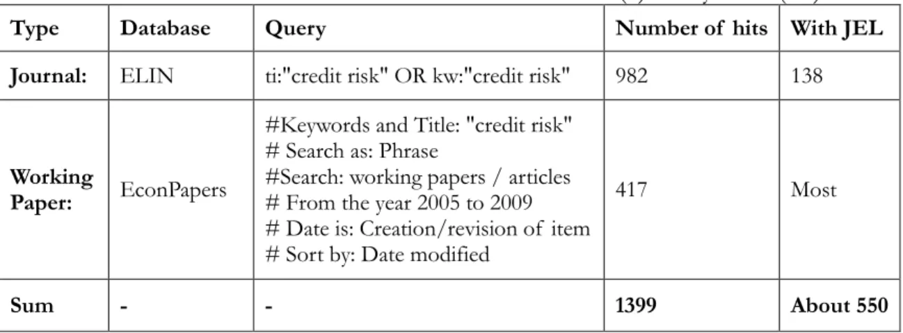
We retrieve articles from these two databases. It yields 1399 hits of articles by April 2009 (see Table 1). We can infer that the 1399 hits include main development in recent 20 years, which is the target of this study.
Table 1 Number of articles with “credit risk” in title (ti) or keywords (kw) Type Database Query Number of hits With JEL Journal: ELIN ti:"credit risk" OR kw:"credit risk" 982 138
Working
Paper: EconPapers
#Keywords and Title: "credit risk" # Search as: Phrase
#Search: working papers / articles # From the year 2005 to 2009 # Date is: Creation/revision of item # Sort by: Date modified
417 Most
Sum - - 1399 About 550
However, it is a challenging task of reviewing and summarizing such a large number of articles within one paper and another problem is that there are many articles of the hits unrelated to credit risk modeling. Therefore, we want to define clearly which articles are supposed to be reviewed before the summarizing work. The words “define clearly” here contain two meanings. First, we should define a criterion to justify which ones are the most interesting in this review. Second, a practicable approach to filter out those unconcerned articles should be formulated here. Usually, the goals can be achieved through adding the important keywords or conditions in our database queries. We do a similar thing but by utilizing the Journal of Economic Literature (JEL) classification code1. But a problem rises here: how do we know which JEL codes, keywords, or conditions are important and relevant to our review?
To solve this question, this paper seeks help from the fundamental idea in statistics. It identifies the 1399 papers, analyzes the relation between the JEL codes and our
preferences among articles in the observable random sample and then infers the population. A statistical model is established to link the dependent variable, our preference rank of the article, to the independent variable, its JEL codes. Because the dependent variable is an ordinal, an appropriate assumption may be a proportional odds model (PO model, also known as the ordered logit model or the ordered logistic regression). In brief, the selection follows five steps.
(i) Sample 40 papers without replacement from the 982 ELIN articles and another 40 from the 417 EconPapers articles.
(ii) Evaluate and rank the 80 papers to divide them into four preference categories. To have a justified article evaluations, the three authors did this work independently, with blinded ranking and resolution to the nonconsensual ranks. Our evaluation standard is as follows.
The rank 0 (= Not interesting) states the paper is “not related to credit risk measurement”. The papers with ranks 1 (= Of little interest) are “in the area of credit risk measurement”, but little related to credit risk modeling or not related to loan credit risk. The papers with ranks 2 (= Interesting) are “about loan credit risk modeling, but with shortcomings or missing some important details to understand the methodology”. Only the ones with ranks 3 (= Very interesting) are “worthy to be reviewed”.
(iii) Extract the JEL classification codes from each article in the sample. (iv) Estimate a proportional odds model, which can be written as
) exp( 1 ) exp( ) ( x β x β T T − − − = ≤ j j j Y P
α
α
where Y represent the preference ranks, j = 0, 1, 2, 3, and x represents the JEL codes. (v) Do inference and forecast the ranks of the 1399 minus 80 articles.
Now, let us come back to the issue why we use JEL codes rather than keywords as the independent variables of the model. This is because of three reasons. First, in the recent 10 years, a classification method according to the system used by the Journal of Economic Literature becomes dominant in economic articles, including the ones on credit risk modeling. The JEL codes, which use three digits to represent the categories, subcategories and subsubcategories of the economic study, provide helpful information and an effective way of reference. So we consider the JEL codes of an article as an important factor related to paper selection, and believe that we can narrow our search based on JEL codes. Second, compared with keywords, there are some distinctive advantages of JEL codes. This is a standard classification and the number of kinds of JEL codes is countable. These merits make JEL codes more suitable for considering as variables in model than keywords. Finally, although that not all the articles have JEL codes is the biggest defect of this method that, our result based on the PO model shows articles without JEL codes is with significantly lower likelihood to be interesting. Because of the consideration of efficiency and feasibility, articles without JEL codes will not be reviewed in this article.
Thus, we create three indicator variables into our regression model. First, we denote variable S1 the set of JEL codes {C14, C15, C23, C24, C32, C4, C5}. If an article
contains at least one JEL code in this set, we say S1=1, otherwise S1=0. Second, variable
S2 denotes another set {(G21 and G28), (G21 and G33)}. If an article includes at least
one group, we say S2=1, otherwise S2=0. Third, we use variable NoJEL to show whether
an article is labeled by JEL codes. NoJEL=1 suggests an article without JEL codes and 0 means it has codes.
According to the result of the ordered logistic regression, we hold following conclusions.
On the one hand, within the articles having “credit risk” in their keywords or titles, the ones with S1=1 or S2=1 have significantly higher possibility to be very interesting. In the
sampled 80 articles, only 19 (23.8%) articles are “very interesting”. In contrast, there are 20 papers in the sample if we search “S1=1 OR S2=1”, and 14 (70.0%) among them are
“very interesting”. Thus, our selection methodology makes the likelihood of finding interesting papers increase from 24% to 70%.
On the other hand, most of the “very interesting” articles satisfy the condition S1=1
or S2=1. There are 19 papers in the top of preference rank, but only 15 have JEL codes.
This means 14 (93%) of them are included in the group with S1=1 or S2=1.
3. Selected articles
3.1 Selection result
Summarizing the above two conclusions, the final result is that we review articles where “(‘credit risk’ appears in keywords or titles) AND (the JEL codes are assigned) AND (S1=1 OR S2=1)”. The last query means the articles have the codes (C14 OR C15 OR
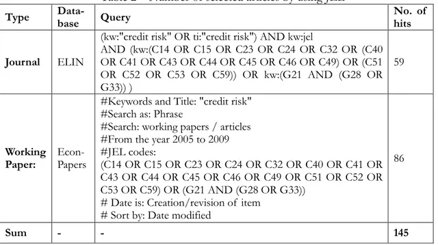
C23 OR C24 OR C32 OR C4 OR C5) OR (G21 AND (G28 OR G33)). Table 2 summarizes the outcome of this selection process. We find 59 published articles in ELIN and 86 working papers dated between the years 2005 to 2009 in EconPapers. As a consequence, the total number of articles in the literature pool decreases from 1399 to 145.
Table 2 Number of selected articles by using JEL Type
Data-base Query
No. of hits
Journal ELIN
(kw:"credit risk" OR ti:"credit risk") AND kw:jel
AND (kw:(C14 OR C15 OR C23 OR C24 OR C32 OR (C40 OR C41 OR C43 OR C44 OR C45 OR C46 OR C49) OR (C51 OR C52 OR C53 OR C59)) OR kw:(G21 AND (G28 OR G33)) ) 59 Working Paper: Econ-Papers
#Keywords and Title: "credit risk" #Search as: Phrase
#Search: working papers / articles #From the year 2005 to 2009 #JEL codes:
(C14 OR C15 OR C23 OR C24 OR C32 OR C40 OR C41 OR C43 OR C44 OR C45 OR C46 OR C49 OR C51 OR C52 OR C53 OR C59) OR (G21 AND (G28 OR G33))
# Date is: Creation/revision of item # Sort by: Date modified
86
Sum - - 145
3.2 Article classification
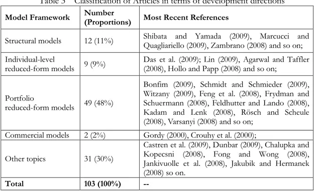
After eliminating 34 unrelated papers (23%) and 9 (6%) articles appearing in both databases, there are 103 of the above 145 articles to be review. Many methods can be
applied to classify these papers. For example, the articles can be divided into empirical studies and theoretical studies; and according to the model inputs, some authors note there are accounting-data-based models, market-data-based models and macroeconomic-data- based models (Bonfim (2009)). Although various classification suggestions are proposed, a consensus has emerged in recent 10 years. Modern credit risk models can be generally classified into “structural models” and “reduced form models” (Saunders and Allen (2002)). We also follow this taxonomy in our work.
The classification of articles is illustrated in Table 3 and a complete listing of the reviewed papers is in the reference.
Table 3 Classification of Articles in terms of development directions Model Framework Number
(Proportions) Most Recent References
Structural models 12 (11%) Shibata and Yamada (2009), Marcucci and Quagliariello (2009), Zambrano (2008) and so on; Individual-level
reduced-form models 9 (9%)
Das et al. (2009); Lin (2009), Agarwal and Taffler (2008), Hollo and Papp (2008) and so on;
Portfolio
reduced-form models 49 (48%)
Bonfim (2009), Schmidt and Schmieder (2009), Witzany (2009), Feng et al. (2008), Frydman and Schuermann (2008), Feldhutter and Lando (2008), Kadam and Lenk (2008), Rösch and Scheule (2008), Varsanyi (2008) and so on;
Commercial models 2 (2%) Gordy (2000), Crouhy et al. (2000); Other topics 31 (30%)
Castren et al. (2009), Dunbar (2009), Chalupka and Kopecsni (2008), Fong and Wong (2008), Jankivuolle et al. (2008), Jakubik and Hermanek (2008) so on.
Total 103 (100%) --
Structural models, also known as asset value models or option theoretic models, spring from Black and Scholes (1973) and Merton (1974)’s work, in which default risk of debt is viewed as the European put options on the value of a firm’s assets and a default happens if a firm’s assets value is lower than debt obligations at the time of maturity. The term “structural” comes from the property that these models focus on the company’s structural characteristics such as the asset volatility or leverage. The relevant credit risk elements, such as default and losses given default, are functions of those variables.
Unlike structural models, the models without examining underlying causalities of default are called reduced-form models. Reduced-form models argue that default time is a stopping time of some given hazard rate process and the payoff upon default is specified exogenously. An incomplete list of early studies on this approach contains Jarrow and Turnbull (1992, 1995), Lando (1994), Duffie and Singleton (1997), Jarrow et al. (1997) and Madan and Unal (1998).
We will explain their detailed evolution in Sections 5, including the recent research progress on traditional credit risk models, which Altman and Saunders (1998) refers to as “credit scoring system models”, as well. However, it should be noted that the credit scoring system models are also a kind of reduced-form models. We name them “individual-level reduced-form models” to distinguish them from the last paragraph mentioned reduced-form ones which focus on loan portfolio defaults.
It should also be mentioned that, the models developed by commercial companies such as the KMV model, CreditRisk+ model and CreditPortfolioView2, are not covered
in this taxonomy. This is not only because of the distinction between them and academic models but also because of the lack in transparency in techniques of commercial model. Actually, based on the table 3, our selected articles include only two papers focusing on the commercial models and both are from the ELIN database in relative earlier years. Thus, we will not discuss these models in this paper, although we agree that these models do significant contributions to credit risk modeling. Details of these models can be found in Gordy (2000) and Crouhy et al. (2000).
3.3 The broad trend
When we take a look into the article distribution in Table 3 and the appended article title list, two salient changes are found. Altman and Saunders (1998) noted that earlier works on credit risk modeling were characterized by a dominant focus on “credit scoring” and “static assessment of default probabilities”. However, neither the situations are held in recent articles. Recent focuses on credit risk modeling move from the individual level to the loan-portfolio level and from static model to the dynamic model. That occurs given the internal needs of credit risk management as well as the availability of more and more historical default data.
4. Databases used in model building and checking
In contrast to bonds, bank loans are usually not traded (with United States as an exception). In additional, the bank’s privacy policy may also be a difficulty in data collecting. As a consequence, database used in modeling credit risk of loans are relatively limited.
Generally speaking, there are two main kinds of databases used in building and checking credit risk models. One is worldwide commercial databases from risk rating agencies. These databases have long time series and large number of observations. For example, Standard and Poor’s (S&P) CreditPro database built from the year 1981 and gives default data and ratings migration data covering more than 13,000 companies, 115,000 securities, 130,000 structured finance issues, and more than 100 Sovereign ratings.3 Moody’s KMV Credit Monitor database is from the early 1990s and provides
the credit exposures, expected default frequencies, asset values or asset on over 27,000 public companies and some private companies in a portfolio.4 Bureau van Dijk Electronic Publishing’s (BvDEP) BankScope database combines data from Fitch Ratings and nine other sources, and now it includes information on 29,000 banks around the
2
Both Crouhy et al. (2000) and Gordy (2000) compared these different commercial models in their articles. Unlike CreditMetrics, KMV does not use Moody’s or S&P’s statistical data to assign a probability of default which only depends on the rating of the obligor. Instead, KMV derives the actual probability of default and the Expected Default Frequency (EDF), for each obligor based on a Merton (1974)’s type model, of the firm.
CreditRisk+ applies an actuarial framework for the derivation of the loss distribution of a loan portfolio. Only default risk is modeled, not downgrade risk. Contrary to KMV, default risk is not related to the capital structure of the firm.
CreditPortfolioView is a multi-factor model which is used to simulate the joint conditional distribution of default and migration probabilities for various rating groups in different industries, It is based on the observation that default probabilities, as well as credit migration probabilities, are linked to the economy..
3
Product web site of CreditPro see, http://creditpro.standardandpoors.com/
world.5 But a shortcoming for these commercial databases (except the BankScope) is that
they are dominated by North American banking system, and the loans for large companies are in the majority. For example, the proportion of the North American loans in CreditPro was 98% in 1980s, although now it decreased to 63%. (Frydman and Schuermann (2008)). Thus, if researchers aim to study the global situation of credit risk or the defaults from small companies, these databases may not be suitable.
Nowadays, it is still common for studies using this kind of databases and the proportion is at least 50% among all the researches. For instance, in all the empirical articles published from 2005 to 2009, there are 9 of 15 studies using commercial databases. S&P’s CreditPro are used by Feng et al. (2008), Frydman and Schuermann (2008), McNeil and Wendin (2007), Ebnöther and Vanini (2007), Lucas and Klaassen (2006) and Hui et al. (2006). Schmidt and Schmiederb (2009) and Kadam and Lenk (2008) use Moody’s database. Lin (2009) uses BankScope database to target 37 listed banks in Taiwan over the time period of 2002-2004.
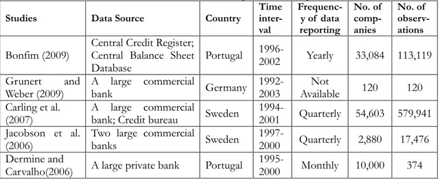
Most of the other studies tend to use the second kind of databases, the data sets collected from commercial banks directly or provided by Central Credit Register, which is credit risk database managed by a country’s central bank. The availability of this kind of databases is increasing especially in Europe. Studies of them cover Czech Republic, Finland, France, Germany, Greece, Italy, Portugal, Sweden Switzerland as well as United Kingdom. By surveying the empirical articles published from 2005 to 2009 again, we have a list in following table (see table 4).
Table 4 Direct commercial banks’ data used in published empirical articles 2005 - 2009
Studies Data Source Country
Time inter- val Frequenc-y of data reporting No. of comp-anies No. of observ-ations Bonfim (2009)
Central Credit Register; Central Balance Sheet Database Portugal 1996- 2002 Yearly 33,084 113,119 Grunert and Weber (2009) A large commercial bank Germany 1992- 2003 Not Available 120 120 Carling et al. (2007) A large commercial
bank; Credit bureau Sweden
1994-
2001 Quarterly 54,603 579,941 Jacobson et al.
(2006)
Two large commercial
banks Sweden
1997-
2000 Quarterly 2,880 17,476 Dermine and
Carvalho(2006) A large private bank Portugal
1995-
2000 Monthly 10,000 374 Although most databases in the second kind are built during the late 1990s or 2000s, which are much later than the S&P’s CreditPro, this inferiority will become less and less influential in further studies. Within the recent five-year studies basing on them, 30% obtain panel data with a more than 10 years interval and 85% more than 5 years. At the same time, these databases usually contain monthly information of loans granted to not only public firms but also private firms and households, including much detailed information not available in commercial databases (such as, whether credit has become overdue, whether it was written-off banks’ balance sheets, whether it was renegotiated and whether it is an off-balance sheet risk), in order to improve their internal credit risk management. Such features for that sort of datasets allow us more facilities for studies on credit risk in those small and medium enterprises and in Europe.
Significant improvement in longitudinal data can still be foreseen in the following years. These data allow us to consider multiple business cycles into credit risk models, which lead to the developments in dynamic models.
5. Risk measures
During the past 10 years, most approaches in credit risk modeling involve the estimation of three parameters: the probability of default (PD), the loss given default (LGD) and the correlation across defaults and losses (Crouhy et al. (2000)). Actually, the first two are identified as two key risk parameters of the internal rating based (IRB) approach, which is central to Basel II. The IRB approach allows banks to compute the capital charges for each exposure from their own estimate of the PD and LGD. Although default and loss are universally acknowledged as critical terms of credit risk modeling, there are no standard definitions for them. We find their definitions and measurements to differ in the articles. To summarize and combine results from the various papers, it is necessary for us to have an overall understanding in the distinctions of the definitions being used.
5.1 Default
The definition of default expressed by the Bank for International Settlements (BIS) is not a clear statement. According to it, default corresponds to the situation when the obligor is unlikely to pay its credit obligations or the obligor is past due more than 90 days on any material credit obligation. Many academic articles, such as Chalupka and Kopecsni (2008), Bonfim (2009) and Schmit (2004), follow the second part of this definition. However, some of the obligors may naturally happen to pay all their obligations back even after 90 days. Particularly in the case of retail clients, days overdue may just be a result of payment indiscipline, rather than a real lack of income to repay the loan. It means a problem of this definition that defaults do not necessarily imply losses.
Some other articles consider default to occur when and only when obligor is “reorganization” bankrupt. This definition is based on United States Bankruptcy Code, which is often referred as “Chapter 11 Bankruptcy”. Some studies on European data also apply the similar definition, basing on their own bankruptcy law. Examples for this group are mentioned in Grunert and Weber (2009) and Agarwal and Taffler (2008). In the option theoretic models, default probability is justified as the probability that obligor’s asset value fall below the value of liabilities, that is, probability of bankruptcy. However, again, a firm can default on the debt obligations and still not declare bankruptcy. Hence, it depends on the negotiations with its creditors. There is still no consensus on the debate over the best definition.
5.2 Losses given default
Another key issue in credit risk modeling is about the LGD or, equivalently, the recovery rate (RR). LGD is usually defined as the loss rate on a credit exposure if the counterparty defaults. It is in principle one minus RR, but also comprises the costs related to default of the debtor. However, because the costs is only a small part of losses, RR and LGD are always used the same conceptually in academic studies.
Therefore, its value is determined by the measuring methods of LGD on individual level and the choice of average weights. Various methods in the both aspects applied by previous researchers are summarized within some studies, e.g. Chalupka and Kopescsni (2008)’s work. It should be noted that, choices of individual LGD measurement and weights in a research should depend on its data availability, hence all the below mentioned concepts are indispensable in recovery estimation.
There are three classes of LGD for individual loan or instrument, referred to as market, workout and implied market LGD. The first one, market LGD, is estimated from market price of bonds or tradable loan when default events occur. But since after-default market is only available for the corporate bonds issued by large companies and bank loans are traditionally not tradable, this approach is highly limited in application. Therefore, most empirical articles for LGD of bank loans, such as Schmit (2004), Dermine and de Carvalho (2005) and Grunert and Weber (2009), suggest applying the second approach, say, workout LGD. It is calculated from the recovered part of the exposure arising in the long-running workout process, discounted to the default date. However, the disadvantage for this approach is that bankrupt settlements are common not only in cash but also with some assets without secondary market. It means that the cash flow generated from the workout process may not be properly estimated. Moreover, the work of selecting appropriate discount rate is difficult as well. The last method is called implied market LGD, which is estimated from market value of risky but non-defaulted bonds or bank loans by using theoretical asset pricing model. Thus, it is naturally applied in the articles related to structural or reduced-form models. It should be emphasized that there is a clear distinction between this approach and the other two: the first two kinds of LGD are hard to estimate before actual default happen or highly rely on historical default; while the estimation of implied market LGD does not rely on historical data so much and is suitable for the studies on the low-default loans or bonds, which do not have sufficient historical losses data.
Additionally, one can also appoint the average weights of LGD in different approaches. Chalupka and Kopescsni (2008) summarized four approaches. They pointed out that portfolio average LGD can be decided to be default count averaging or exposure weighted averaging, and to be default weighted averaging or time weighted averaging. The formulas of portfolio average LGD calculated in the four kinds of weights are available in their paper. In practice, default weighted averaging is more frequently used than time weighted averaging. And default count averaging is usually recommended to be used in studies on non-retail segment. In contrast, retail portfolios and some small and medium-sized enterprises (SME) loans apply exposure weighted averaging.
6. Credit risk models
In the previous section, we summarized the outcome variables which are modeled by existing literature on credit risk. However, it seems more logical that the articles should be reviewed according to their modeling framework.
Three broad categories, being structural model, individual-level reduced-form model and portfolio reduced-form model, are introduced in this part. However, we want to point out that when we reviewed the recent articles, one kind of cross model attracted our attentions. This kind of model assumes defaults to follow an intensity-based process, with latent variables that may not be fully observed because of imperfect accounting and market information (Allen et al. (2004)), and default happens when the latent variables
fall behind a threshold value. Thus, this kind of model stems from both structural modeling and reduced-form modeling framework. Nevertheless, to review effectively, we put this kind of model in the sub-category of portfolio reduced-form models, titled and refer to it as “factor model”.
6.1 BSM framework structural models
As mentioned before, the idea of this kind of model is proposed by Merton (1974). Merton (1974) derived the value of an option for a defaultable company. In the classical Black-Scholes-Merton (BSM) model of company debt and equity value, it is assumed that there is a latent firm asset value A determined by the firm’s future cash flows, where A follows Brownian motion. Its value at time t, given by At , satisfies
t A A t t dz t dt t r A dA ) ( ) ( +
σ
=Where rA (t) and σA (t) denote asset return rate (rA (t) contains there components:
risk-free interest rate r, asset risk premium λand asset payment ratio δ) and volatility of asset value, zt follows the standard Wiener process and dzt is standard normally
distributed. In Merton’s (1974) work,rA (t) and σA (t) are constants and non-stochastic.
And he assumes the firm’s capital structure just relate to two things: pure equity (that means preference stocks are not considered) and a single zero-coupon debt maturing at time T, of face value B. The default event only occurs when the asset value at maturity is less than B. Upon the random occurrence of default, the stock price of the defaulting company is assumed to go to zero. Thus, we have the following payment equations
− = = ) 0 max( holders equity of Receives ) min( holders debt of Receives B, A ,B A T T
Thus, debt holder can be considered as a seller of European put option, equity holder can be considered as a buyer of European call option in Merton’s (1974) work and asset value A can be considered as the price of underlying security. By assuming there are no dividends, we can use standard Black-Sholes option-pricing equation to get a relation between the equity market value Et and At and the bond market value Yt and At. In
general form, that is,
= = ) ), ( , , , ( ) ), ( , , , ( 2 1 T t r B A f Y T t r B A f E A t t A t t
σ
σ
where r means short-term risk-free interest rate and the meaning of other variables are as mentioned before. Variables which have a bar above them are observable and exogenous. However, according to Modigliani-Miller Theorem I (1958), it holds that Et +Yt = At in any capital structure, any one of the above two equations can be derived from the other. It means that we actually do not need to calculate the second one. As Delianedis and Geske (1998) discussed, there should be linkage between observable stock volatility σt and unobservable asset volatility σA (t), so if we specify the form of this linkage
)) ( ( ) (t g A t E σ
σ = (e.g. many articles directly use σE (t) to substitute σA (t)), Yt and At can
be known.
The biggest disadvantage of Merton’s (1974) model is that there are too many simplified assumptions for its derivation. These simplifications restrict the applied value of the model. Thus, its subsequent researches mainly focus on relaxing these assumptions.
The one most worthy to be elaborated is maturity. We find three kinds of extending methods for it in our review. First, Geske (1977) extended the original single debt maturity assumption to various debt maturities by using compound option modeling. Second, in Leland and Toft (1996)’s work, firms allow to continuously issue debts of a constant but infinite time to maturity. Last but not least, Duffie (2005) mentioned that, compared with Merton (1974)’s assumption that the default occurs only at the maturity date, another group of structural models is developed by Black and Cox (1976). The models are often referred to as “first-passage-time model”. In this class of models, default event can happen not only at the debt’s maturity, but can also be prior to that date, as long as the firm’s asset value falls to the “pre-specified barrier” (that is, default trigger value). Thus, the models not only allow valuation of debt with an infinite maturity, but, more importantly, allow for the default to arrive during the entire life-time of the reference debt or entity.
Staying with this first-passage-time idea, other parameters that Merton assumes constant are also extended to be dynamic. For example, Longstaff and Schwartz (1995) treated the short-term risk-free interest rate as a stochastic process which converges to long-term risk-free interest rate and is negatively correlated to asset value process, so that the effect of monetary policy to macro economy are considered.
Additionally, the default barrier Bt is also treated dynamically in various papers. Briys
and Varenne (1997) assumed that the change of Bt follows the change of risk-free
interest rate rt . Hui et al. (2003) argued that default barrier should decrease when time
goes, because they observe that there is high default risk at time close to maturity. Collin-Dufresne and Goldstein (2001), based on their observation that firms tend to issue more debt when their asset value increases, proposed that the default trigger value
Bt, which is considered as a fixed face value of debt in Merton model, should be a
process converging to a fraction of asset value At. Actually, this model implied a
widespread strategy that firms tend to maintain a constant leverage ratio. Hui et al. (2006) developed this stationary-leverage-ratio model to “incorporate a time-depending target leverage ratio”. They argued that firm’s leverage ratio varies across time, because of the movement of initial short-term ratio to long-term target ratio as stated in Collin-Dufresne and Goldstein (2001). Their model assumed default occurs when a firm’s leverage ratio increases above a pre-specific default trigger value and the dynamic of interest rate follows the set of Longstaff and Schwartz (1995). By doing so, the model captures the characters of the term structure of PD, which was mentioned in Hui et al. (2003).
Furthermore, Huang and Huang’s (2003) model postulated that the asset risk premiums λt is a stochastic process and that there is negative correlation between it and
the unexpected shock to the return of asset value. They include the empirical finding which says that risk premiums of a security tend to move reversely against the returns of stock index in it.
There is another classification of the family of structural models. The models can be divided into exogenous default group and endogenous default group (Tarashev (2005)). The distinction between these two groups is somewhat related to the two definitions of default in the Section 5.1. All the above mentioned works belong to the former group, in which default is defined as when the asset value fall below a trigger value. While the endogenous default models allow obligors to choose the time of default strategically, for which default also depends on negotiation. For example, the latter group of models contains Anderson et al. (1996). Anderson et al. (1996) allowed firms to renegotiate the terms of debt contract. When default trigger value is touched, a firm can either declare
bankruptcy or give a new but higher interest rate debt contract to debt holder. An empirical comparison of these two groups of model can be found in Tarashev (2005).
The last noteworthy BSM structural model was proposed by Shibata and Yamada (2009). They developed BSM structural model to model bank’s recovery process for a firm in danger of bankruptcy. When obligor bankrupts, the bank’s choice whether the firm should be run or be liquidated affects the losses of the loan. Shibata and Yamada (2009) assumed this decision is made at continuous time t after the bankruptcy. Using this option approach and incorporating the application of game theory, the paper described the property of the bank’s collecting process.
6.2 Individual-level reduced-form models
We define all the models not belonging to the class of structural models as being reduced-form models. The individual-level reduced form model is commonly called as credit scoring system or credit scoring model. As we will show bellow, only a small share of the articles (less than 9%) fully study this issue. Hence, we do not cover the topic extensively, rather than present some important developments in that field.
The credit scoring model was proposed by Altman (1968). By identifying accounting variables that have statistical explanatory power in differentiating defaulting firms from non-defaulting firms, this approach uses linear or binomial (such as logit or probit) models to regress the defaults. And once the coefficients of model are estimated, loan applicants are assigned a Z-score to classify they are good or bad.
This individual-level model got significant development in the decades after its proposal. Earlier results of this issue are discussed in some overview studies at the end of 1990s comprehensively. Altman and Saunders (1998) mentioned the widespread use of credit scoring models as well as the model developments. Altman and Narayanan (1997) surveyed the historical explanatory variables in credit scoring models throughout the world. They found that most of the studies suggest the use of financial ratios which measure profitability, leverage and liquidity, such as Earnings Before Interest and Tax (EBIT)/sales, market value equity/debt, working capital/debt and so on, in their models. However, the consensus about specific choice of these variables is not made.
Whereas in recent 10 years, articles concentrating on credit scoring models are not so many. In our article pool, just 4 papers base on it. Jacobson and Roszbach (2003) build on bivariate probit model and “proposes a method to calculate portfolio credit risk” without bias. Lin (2005) proposed a new approach by three kinds of two-stage hybrid models of logistic regression-artificial neural network (ANN). Altman (2005) specified a scoring system, namely Emerging Market Score Model, for Emerging Corporate Bonds, which is not much related to out topic. The last one is Luppi’s et al. (2007) work. They applied logit model to Italian non-profit SMEs and found that traditional accounting-based credit scoring model held less explanatory power in non-profit firms than that in for-profit firms.
One of the main criticisms about credit scoring models is that because their predominant explanatory variables are based on accounting data, these models may fail to pick up fast-moving changes in borrower conditions. Many studies, of which an incomplete list is given in Agarwal and Taffler’s (2008) paper, test this argument. Those studies successfully showed that the market-based model such as structural models are better at forecasting distress than credit scoring models such as Altman’s Z-score, although we also found two recent papers obtain a reversed result. Agarwal and Taffler
(2008) manifested that in term of predictive accuracy by using the data of UK, their results are almost same from their two different specified BSM structural model and the Z-score model. Moreover, they pointed out that, if considering differential misclassification costs and loan pricing considerations, Z-score model has greater bank profitability. Das et al. (2009) also found these two kinds of models perform comparably. But, no matter which kind of the results is, it has been a fact that more interests have been brought to dynamic portfolio model from this purely static and individual-level credit scoring model.
6.3 Portfolio reduced-form models
Similar to the situation of structural models that the structural models become popular after their introduction by commercial firms such as KMV in 1990s, PD calculated by portfolio reduced-form models have been growing rapidly in popularity since the early 2000s (Das et al. (2009)). Actually, in recent contributions, there are around 50% papers based on this kind of model.
These models were originally introduced by Jarrow and Turnbull (1992) and widely mentioned by later studies. Jarrow and Turnbull’s (1992) idea behind these models is highly associated with the concept “risk neutral”, which in finance means a common technique to figure out the risk neutral probability of a future cash flow and then to discount the cash flow at the risk-free interest rate. One can calculate of asset prices by utilize risk neutral default probabilities. Based on this statement, Jarrow and Turnbull (1992) decomposed the credit risk premium, which can also be called credit spread, in two components, PD×LGD, and then the core problem of credit risk modeling becomes to model the distributions of PD and LGD.
Although structural models are very attractive because of their fine theoretical bases, in empirical studies, reduced-form models are reported to perform better to capture the properties of firms’ credit risk. By specifying different stochastic process models, this kind of models can be subdivided into various subclasses. In this paper, we discuss four subclasses, which are most common appeared in our selected articles.
6.3.1 Poisson / Cox process model
This framework is referred to by Gaspar and Slinko (2005) as “doubly stochastic marked point process”. In fact, these two names have the same connotation. Since Cox process is also known as “doubly stochastic Poisson process” and “marked point process”, which is more commonly called as counting process. It is a generalization of Poisson process. About 8% articles are based on Poisson/ Cox process model.
Poission model is the simplest model of reduced-form consideration, which was proposed by Jarrow and Turnbull (1995). In that work, the default process is modeled as a Poisson process N(t) with constant intensity λ, in which default time τ is exponentially distributed as a consequence. They also assumed RR as a fixed value. However, it is a somewhat strong assumption that the intensity λ is constant over time and across the loan clusters (e.g. across different credit ratings or industries). Another similar shortcoming lies in its assumption of RR. In reality, RR is neither fixed over time nor independent with default rate. Thus, the earlier works about reduced-form model put a lot of concerns to modify these two assumptions.
Two main methods are employed to extend the assumption of λ(t). One is as what was done by Madan and Unal (1998). They assign the intensity λ(t) to be a function of the excess return on the issuer’s equity. A similar idea is applied in Duration models, which were mentioned by Carling et al. (2007). To allow the intensity vary over time and differ across the loans’ properties, in practice, it is natural to consider default intensities depending on some observable variables which affect PD. These variables can be accounting variables such EBIT/Asset, market variables such as market equity price, macroeconomic variables such as GDP index, and other variables such as duration of loan. Carling’s et al. (2007) model considered all these kinds of variables, by assuming that a linear relation is held between the selected variables and the log value of intensities. They found that accounting variables and macroeconomic variables are most powerful to explain the credit risk.
The other kind of approach is to modify λ(t) to a stochastic process, e.g. Cox process model which was proposed by Lando (1998). The default time τ in this model is treated as the first jump time of a Cox process. That is, τ is the infimum of the following set.
{
0}
inf ∈ >
= t R+ N(t)
τ
where N(t), the Cox process, generalizes a Poisson process with time-dependent and stochastic intensity λ(t). In Lando’s (1998) case, it is defined as follow.
t dW t dt t t) ( ) ( ) ( µλ σλ λ = +
The equation shows Lando (1998) assume λ(t) to be Brown motion. µλ (t) and σλ (t) are mean and volatility of the intensity; Wt is a standard Wiener process where
) 1 , 0 ( ~ N
dWt . Alternative distributions are assumed in other articles as well. Gaspar and Sliko (2005) proposed a model where both PD and LGD are dependent on market index, which is log-normally distributed, and therefore the correlation between PD and LGD can readily be computed.
6.3.2 Markov chain model
To the authors’ knowledge, applying this kind of model to credit risk was first mentioned in Jarrow et al. (1997). The Markov chain model considers default event as an absorbing state and default time as the first time when a continuous Markov Chain hits this absorbing state. In Jarrow’s et al. (1997) model, they assumed fixed probabilities for credit quality changes, which is estimated from historical credit transition matrices, and a fixed RR in the event of default. These time-homogenous discrete-time Markov chain models are widely used (Bangia et al. (2002)). Several developments of Markov chain model are made. There are 11 recent papers from our selection in this group.
First, similar to Poisson process model, there are also modifications for the homogeneous assumption. However, this modification is focusing on rating transition probabilities, rather than the intensity in the above section.
One of the key models here is ordered probit model. Nickell et al. (2000) and Feng et al. (2008) fitted ordered probit model to rating transition. The rating transition probabilities are viewed as functions of latent variables. However, the former work assumes latent variables derived by observable factors such as industry, residence of the obligor and variables related to business cycle, while Feng et al. (2008) introduced unobservable factors and argue recent literature on credit risk shows preference for the
use of unobservable factors (related details are shown in the factor model section later). In addition, the ordered probit model can also be applied in sovereign credit migration estimating, as Kalotychou and Fuertes (2006) did. They also do a comparison between homogeneous and heterogeneous estimators. Gagliardini and Gourieroux (2005) applied ordered probit model for another aim: to estimated migration correlations. They also point out that the traditional cross-sectional estimated migration correlations are inefficient.
Monteiro et al. (2006) suggested using “finite non-homogenous continuous-time semi-Markov process” to model time-dependent matrices. As the definition, semi-Markov process is a Markov chain with a random transformation of the time scale. Monteiro et al. (2006) show that the nonparametric estimators of the hazard rate functions can be used for consistently estimating these time-dependent transition matrices.
Second, Jarrow’s et al. (1997) discrete-time model was commonly extended to continuous-time model. Many papers aim to check Jarrow’s et al. (1997) argument that the results based on discrete-time Markov Chain processes can be improved if we adopt the continues-time ones. Many articles are involved in this topic, such as the contributions made by Monteiro et al. (2006), Fuertes and Kalotychou (2006), Frydman and Schuermann (2008), Kadam and Lenk (2008). Lucas and Klaassen (2006) applied both discrete-time and continuous-time Markov chain model in empirical studies.
At last, although all the above models use Markov Chain process as a core in their framework, their emphases are not on Markovian behaviors but on the non-Markovian behaviors, such as heterogeneous and time-varying rating transition probabilities due to industry class and macroeconomic variables. The literatures which focus on Markovian behavior in credit risk have been exclusively submitted recently. Thus, we divided Markov Chain articles into non-Markovian behavior group and Markovian behavior group. For the latter, there are studies as following.
Hidden Markov Models (HMM) is a statistical model in which the system being modeled is assumed to be a Markov process with unobserved states. It is used to forecast quantiles of default rates in credit risk modeling. Banachewicz and Lucas (2007) did a further study on this area, and tested the sensitivity of the forecasted quantiles if the underlying HMM is mis-specified.
Frydman and Schuermann (2008) and Kadam and Lenk (2008) applied Markov mixture model to their analysis. In their work, the original Markov chain model is extended to a mixture of two Markov chains, where the mixing is on the speed of movement among credit ratings. The main difference of these two works is that the estimation of the former one is based on maximum likelihood method while the latter uses Bayesian estimation.
6.3.3 Factor model
Although the intuitions of structural model and reduced-form model appear significantly different, clear distinction does not exist under some model frame work. Actually, there is no pure “non-structural” model, and as McFadden (1974) stated, even the simplest logit model bears a structural instruction in it. This fact is more obvious in the factor model. Gordy (2000) pointed out structural models (CreditMatric model in his work) can map to reduced-form models (CreditRisk+ model in his work) in some degree under factor
models framework.Regardless of the different distributions and functional forms these two kinds of models assume, both of them actually use the similar correlation structures that the correlation between defaults is totally driven by some specific common risk factors, which can be called as “systematic factors”.
Partly because of IRB approach in Basel II, factor models are most widespread in current literature. About 25% papers in literature pool follow this framework. In these models, the default event of firm i in period t is modeled as a random variable Yit so that
= otherwise 0 in defaults firm if 1 i t Yit And hazard rate is defined as
) 1 Pr( = = it it Y
λ
One of the key characters of factor models is that they model hazard rate through one or a set of latent variables, which follows the structure model’s idea: the obligor will default if latent variables fall below a given threshold Cit. Usually the latent variable is the
firm’s returns rate Rit., however, some papers use firm’s asset value Ait as latent variable
( Kupiec (2007a)). In the common cases,
) ( Pr ) 1 Pr( it it it it = Y = = R ≤C
λ
Factor models often consider two vectors of explanatory variables for latent variable. The first one (
X
it) is a set of macro-economical variables, such as GDP growth, interestrate, money supply growth, inflation rate, stock index and firm’s industry as well. This vector intends to explain systematic risk, which leads the correlations of default events. The second vector is a set of firm-specific variables (
Z
it,) which account for individualrisk. This vector may include contemporaneous and lagged variables regarding several dimensions of the firm’s property, such as age, size, asset growth, profitability, leverage and liquidity.
Some models, such as Pederzoli and Torricelli (2005) and Borio et al. (2001), considered these variables simultaneously. These models are called multi-factor models. These models assume that, set
ε
it as error termit it it it X Z R =Γ +∆ +
ε
Thus,(
,)
( ) Pr it it it it it it it it it it = ΓX +∆Z +ε
≤C X Z = F C −ΓX +∆Zλ
where F(.) is cumulative distribution function of the error term
ε
it.However, it is more popular to use only one systematic random factor to model credit risk, and consider individual risk as a non-deterministic random variable. In these models, defaults are assumed to be driven by the single systematic factor, rather than by a multitude of correlated factors. These one-factor models, which are also called single-factor models, were mentioned in works of Altman et al. (2004), Diesch and Petey (2002, 2004), Repullo and Suarez (2004), Ebnöther and Vanini (2007) and Witzany (2009) and so on. They follow the IRB approach which utilizes a one factor model to calibrate risk weights. Additionally, these models always base on the assumption that the economic conditions which cause defaults to rise might also cause LGD to increase.
They model both PD and LGD dependent on the state of the systematic factor. The intuition behind factor model is relatively simple: if a borrower defaults on a loan, a bank’s recovery may depend on the value of the loan collateral. The value of the collateral, like the value of other assets, depends on economic conditions.
The simplest version of the singled-factor model is probably the model proposed by the Tasche (2004), which assumes both systematic risk factorXit and individual error term
ε
it follow the standard normal distributions, and the sum of their risk weight equals to 1. Conditional PD can be calculated by(
)
) 1 ( ) 1 ( Pr ω ω ε ω ω λ − − Φ = ≤ − + = it it it it it it it X C X C XAnd the unconditional PD, that is, long term PD can be calculated by
(
(1 ))
( )Pr it it it it
it = ωX + −ω ε ≤C =Φ C
λ
It should be pointed out that the square of risk weight of systematic risk factor
ω
2 is also the correlation coefficient between the defaults event.Both in multi-factor model and single-factor model, they always assume the distribution of the error term follows normal distribution, as the above mentioned papers. But there are alternative assumptions of the factors’ distributions. Gordy(2000) and Dietsch and Petey (2002) indicated a factor model where the factors are gamma distributed with mean 1 and variance σ2.
Ebnöther and Vanini (2007) extented the standard single factor model to multi-period framework. That is, latent variables are a set of return rates in different time period. 6.3.4 Mortality analysis
Mortality analysis of loan can also be viewed as a type of reduced-form models, because it is based on the survival time of loan as well. Altman and Suggitt (2000) applied this actuarial method to study mortality rates of obligation. Although before them there were some prior works in the area of credit risk based on mortality analysis, most works concentrate on corporate bonds while Altman and Suggitt (2000)’s study focused on US large bank loan. They find that loans show higher default rates than bonds for the first two years after issuance. This approach was followed by studies on recovery rates, on the probability of default over time for different credit ratings, on recovery rates based on market prices at the time of default, on estimates of rating transition matrices and on the degree of correlation between default frequencies and recovery rates.
The instances in our article pool contain Nickell et al. (2000), Dermine and de Carvalho (2006) and so on. Nickell et al. (2000) studied on the issue that choosing an appropriate survival probability for representative banks over a specific horizon. Dermine and de Carvalho (2006) have applied morality analysis to recovery rate. They found that beta distribution does not capture the bimodality of data.
7. Performance tests of credit risk
There are statistical uncertainties in realized default rates. Therefore, it is important to develop mechanisms to show how well the credit assessment source estimates the losses.
Although only 7 papers specifically focus on this issue, most papers are more or less considering it.
7.1 Statistical tests in credit risk modeling
These evaluating tasks are generally done by using statistical tests to check the significance of the deviation between the realized and in-sample predicted PD (or default frequency). Coppens et al. (2007) have summarized these statistical tests for this purpose. There are extensive articles applying Wald/normal test to test the realized default rates, based on the model assumption that realized default frequency follows a binomial distribution, which could be approximated by a normal distribution. However, Wald test is only suited to testing single default rate, sometimes we need to test several default rates simultaneously, to allow for variation in PDs within the same credit rating or loan cluster, and to take into account default correlations. For these problems, other statistical tests are introduced into this area. Hosmer-Lemeshow test is applied to analyze deviations between predicted probabilities of default and realized default rates of all rating grades or loan clusters, by using the sum of the squared differences of predicted and observed numbers of default, weighted by the inverse of the theoretical variances of the number of defaults as statistic. Spiegelhalter test, which focus on the mean square error (MSE), is used when the probability of default is assumed to vary for different obligors within the rating grade or loan cluster. Tasche (2003) summarized two statistics that considered the correlation between defaults, namely “granularity adjustment approach” and “moment matching” approach, under internal rating based model.
In the context of evaluating VaR models, the test are against losses directly rather than PD. Lopez and Saidenberg (2000) discussed statistical tools used in this issue. For example, they refer likelihood ratio (LR) statistic in binomial method to evaluating the forecasted critical value of losses.
7.2 Test Strategies
There are two strategies to implement the tests in the Section 7.1. One is back test and the other is stress test. Back test (or backtesting) evaluates the model’s expected outcomes based on historical data. Whereas, stress test (or stress-testing) is examine the model’s expected outcomes under extreme conditions.
In recent articles, only Coppens et al. (2007) referred to back test and propose a simple mechanism to check the performance of credit rating system estimate the probability of default by applying traffic light approach, which is a simplified back test incorporating the above mentioned statistical tests in their frame.
In contrast, an amount of studies on stress test have emerged after Basel II requires banks to conduct systematic stress tests on their potential future minimum capital. At its simplest, a stress test on credit risk is performed by applying extreme scenarios of default and bankruptcy, to identify potential risks of banks or banks’ loan portfolios. We run it to test whether the banking system or the loan portfolios can withstand the recession and the financial market turmoil. Two macroeconomic scenarios are constructed in usual. One is based on baseline conditions and the other is with a more pessimistic expectation. The recent stress tests are mostly integrated with macroeconomic credit risk models.
Cihak et al. (2007) provided a brief overview of stress tests applied by the Czech National Bank. They put their emphasis in introducing a model-based macro stress test and derive scenarios according to the forecast. Both Jokivuolle et al. (2008) and
Valentinyi-Endresz and Vásáry (2008) adopted Wilson (1997a, 1997b)’s macro model and generated scenarios though Monte Carlo simulation. Fong and Wong (2008) extended macro stress testing under mixture vector autoregressive (MVAR) model, which assume either default rate or macroeconomic variable is a mixture normal distribution, and apply Monte Carlo simulations as well.
7.3 Evaluation of bank’s Internal Rating
Recent interests of internal rating are mainly from the suggestion of internal rating based (IRB) approach by Basel II and focus on the following two aspects.
One is about how to design specific banks’ internal ratings systems suited to Basel II. For example, Crouhy et al. (2001) suggested how an internal rating system could be organized according to their analysis of standardized external rating system, such as Moody’s and S&P’s. Fernandes (2005) showed the probability to “build a relatively simple but powerful and intuitive rating system for privately-held corporate firms”.
The other aspect is about how the implementation of internal credit rating by banks will lead to differences in minimum capital requirements. Jacobson et al. (2006) compared the loss distributions computed by two of the largest Swedish banks with equally regulatory internal ratings and find that their results are widely different in many cases. They point out these differences may be due to the design of a rating system and the ways in which they are implemented. Van Roy (2005) considered another possible reason for these differences associated with which external rating agency the bank selects. Because implementing the internal rating by banks generally calibrate their assessments to existing external ratings, differences of opinion among external raters may also cause differences of opinion among internal ratings systems and thus lead to different results in internal rating based approach.
8. Studies on SME
Before 2000, few studies have been devoted to modeling credit risk in small and medium enterprises (SMEs) or retail section. The conclusions from the credit risk models were mostly facing to wholesale commercial loans at that stage. This situation is partly because of the data availability, which we have discussed in the Section 4, and it has been changed in recent studies. 5% of all articles concentrate on SME loans study and more empirical study is based on dataset of SME loans. This is not only because of the quickly development of SME loan business, but also the suggestion in Basel II.
Historically, discriminant analysis and logistic regression have been the most widely used methods for constructing scoring systems for SME. Several studies have proposed to use some new models. Bharath and Shumway (2004) employ a time-dependent proportional-hazards model to evaluate the predictive value of the Merton structural model. Dietsch and Petey (2002, 2004), basing on large samples of French and German SMEs, suggested to apply a one-factor ordered probit model to catch properties of further losses in SME portfolio. They show the PD of SME is positively correlated rather than negatively to firm’s asset value. What’s more, both of these two studies mention correlations are weak between the SMEs’ asset prices, especially for the SMEs with small size. Their result suggests that the properties of SME loans differ according to company scale, and there should be size-specified models even if inside SME.
9. Conclusion
During the past decade, two remarkable things happened in the field of credit risk modeling. One is the proposal of Basel II, whose influence have been considered by many researchers, including Repullo and Suarez (2004), Sironi and Zazzara (2003), Riportella et al. (2008) and so on. The other is the increasing availability of longitudinal data opening up for dynamic study on credit risk. These two changes brought important consequences for banks, bank supervisors as well as for the direction of academic works. In this paper, we review the recent development in credit risk modeling, and the main conclusions are in the following.
(i) It can be noted that the current focuses on credit risk modeling have shifted from static individual loan models to dynamic portfolio models. Credit scoring system model is no longer the dominant model in this field. Studies make more efforts to consider the correlations between default and business cycle, and between defaults in portfolios. As a result, macroeconomic variables are added to different modeling frameworks, which reduce the importance of accounting variables.
(ii) Earlier studies only model the PD, while this situation has been reversed in term recent increasing works on LGD and RR. This is partly because the assumption in traditional analysis that LGD is a constant is widely doubted based on recent empirical results. Nowadays, more and more works are dedicated to modeling the distribution of LGD and PD simultaneously and the correlation between them.
(iii) Factor models have increased significantly in the number of applied studies. As a suggestion of internal rating based (IRB) approach in Basel II, factor models, especially, single factor model begin to appear frequently in academic works and step by step become the largest part of studies on credit risk modeling.
(iv) Another observation is that there is an increasing concern on modeling the credit risk of SMEs. The accepted distinction between the properties of retail and cooperate loans lead to the development of sector-specific models.
(v) As we proved in the methodology part, JEL codes have become the standard to classify researches in credit risk modeling.
(vi) A few JEL codes, namely (C14 OR C15 OR C23 OR C24 OR C32 OR C4 OR C5) OR (G21 AND (G28 OR G33)), have historically been used by researchers to label their contribution on credit risk modeling. We suggest use these JEL codes to label the coming studies on credit risk modeling so that the future literature reviews will be easier.
(vii) No consensus on the definitions of the three key parameters, being PD, LGD and correlation has emerged. However, we note that there are some conclusions made on how to choose the definitions of these parameters, according to data availability, property of loan and the objective of the study.