The composition and use of the Swedish car fleet : Formulation of a forecasting system

Full text

(1)VTI rapport 518A Published 2005. www.vti.se/publications. The composition and use of the Swedish car fleet Formulation of a forecasting system Åsa Forsman Inger Engström.

(2)

(3) Publisher:. Publication:. VTI rapport 518A. SE-581 95 Linköping Sweden. Published:. Project code:. 2005. 50740. Project:. The composition and use of the Swedish car fleet – Formulation of a forecasting system Author:. Sponsor:. Åsa Forsman Inger Engström. The emission research programme. Title:. The composition and use of the Swedish car fleet – Formulation of a forecasting system. Abstract (background, aims, methods, results) max 200 words:. Model-based forecasts of future emissions are important tools for finding strategies to reach the Swedish transport policy objective concerning effect on climate and air pollution. In order for the calculated emissions to reflect the actual situation, input data on kilometrage, vehicle types and vehicle ages must be representative of the region of interest. High-quality forecasts of these variables are therefore of great importance when estimating future emissions. This report proposes a forecasting model system for the compositions and use of the Swedish car fleet, based on experiences from existing models in the literature. The system operates on two levels, an aggregated (national or regional) level and a disaggregated (household or personal) level. Forecasts of the total number of cars and total kilometrage are provided from the aggregated models whereas the disaggregated models provide the distribution of cars of different types and ages and the distribution of kilometrage over the same classification of cars. These results are then combined to give the final outcomes: the number and kilometrage of cars of different types and ages.. ISSN:. 0347-6030. Language:. No. of pages:. English. 42 + App..

(4) Utgivare:. Publikation:. VTI rapport 518A. 581 95 Linköping. Utgivningsår:. Projektnummer:. 2005. 50470. Projektnamn:. Den svenska bilparkens sammansättning och användning – formulering av prognosmodell Författare:. Uppdragsgivare:. Åsa Forsman Inger Engström. Emissionsforskningsprogrammet (EMFO). Titel:. Den svenska bilparkens sammansättning och användning – Formulering av prognosmodell. Referat (bakgrund, syfte, metod, resultat) max 200 ord:. Modellbaserade prognoser för framtida emissioner är viktiga verktyg i arbetet med de transportpolitiska miljömålen om klimatpåverkan och luftföroreningar. För att emissionsberäkningar ska spegla faktiska förhållanden krävs att indata i form av körsträckor, fordonstyper och fordonsåldrar är representativa för den region man är intresserad av. Kvalificerade prognoser för dessa variabler är därför av stor vikt när man vill uppskatta den framtida emissionsutvecklingen. I den här rapporten formuleras ett system av prognosmodeller för den svenska bilparkens sammansättning och användning. Systemet baseras på erfarenheter från existerande modeller som beskrivs i litteraturen. Modellerna är indelade i två nivåer, dels en aggregerad nivå (nationellt eller regionalt), dels en disaggregerad nivå (hushåll eller individ). Prognoser för totalt antal bilar och totalt trafikarbete modelleras på den aggregerade nivån medan den disaggregerade nivån ger fördelningen av bilar av olika typ och årsmodell och fördelningen av trafikarbete för samma indelning.. ISSN:. 0347-6030. Språk:. Antal sidor:. Engelska. 42 + bilaga.

(5) Preface Model-based forecasts of future emissions are important tools for finding strategies to reach the Swedish transport policy objective concerning effect on climate and air pollution. In order for the calculated emissions to reflect the actual situation, input data on kilometrage, vehicle types and vehicle ages must be representative of the region of interest. High-quality forecasts of these variables are therefore of great importance when estimating future emissions. As a part of the work of improving the forecasts of future emissions, VTI has carried out a study with the aim of formulating a forecasting model system of the car fleet’s composition and use. The study was founded by the emission research programme (EMFO), and the following persons at VTI have contributed to the work: Inger Engström, Åsa Forsman, Ulf Hammarström, Pontus Matstoms, and Tomas Svensson. Linköping august 2005 Åsa Forsman, project leader. VTI rapport 518A.

(6) VTI rapport 518A.

(7) Contents Summary. 5. Sammanfattning. 7. 1. Introduction and aim. 9. 2 2.1 2.2 2.2.1 2.2.2 2.3 2.4 2.5 2.5.1 2.5.2 2.5.3 2.5.4 2.5.5 2.6. Orientation of existing models and model systems 11 Car ownership 11 Car fleet composition 12 Acquisition of new cars 12 Scrappage 13 Car use 13 Licence holding 14 Some specific model systems 14 The ALTRANS model 14 The COWI Cross-Country Car Choice Model 15 CARMOD 16 FACTS (Forecasting Air pollution through Car Traffic Simulation)17 DVTM (Dynamic Vehicle Transaction Model) 18 Factors included in existing models 18. 3 3.1 3.2. Gaps and shortcomings in existing model systems Limitations of the model systems Absence of motivational factors. 20 20 21. 4. Purchase behaviour and the decision process. 22. 5 5.1 5.1.1 5.1.2 5.1.3 5.2 5.2.1 5.2.2 5.2.3 5.2.4 5.2.5 5.2.6 5.3. A proposition of a new model system Overview Basic concepts Co-ordination with Sampers Summary of the sub-models Description of the sub-models Car ownership (1) Total kilometrage (2) Licence holdings (3) Household car transactions (4) Kilometrage per car (5) Combining aggregated and disaggregated results (6) Forecasts and scenarios. 25 25 26 27 28 29 29 30 31 31 34 35 36. 6. The steps towards a working model. 37. 7. Discussion. 38. 8. References. 40. Appendix: Multinomial and nedsted logit models. VTI rapport 518A.

(8) VTI rapport 518A.

(9) The composition and use of the Swedish car fleet – formulation of a forecasting system by Åsa Forsman and Inger Engström VTI SE-581 95 Linköping Sweden. Summary Model-based forecasts of future emissions are of great importance for analysing and comparing different strategies to reach the Swedish transport policy objective concerning effect on climate and air pollution. The composition and use of the car fleet are important inputs to emission models, and the quality of the emission forecasts therefore depends on the quality of the car fleet forecasts. Today, no Swedish national model system exists that provides all the important forecasts. The aim of this study has been to formulate such a system based on experiences with models described in the literature. The model requirements are summarised in the following list: 1. The model should provide the following outputs: a. Forecasts of the total number of cars in the Swedish car fleet b. Forecasts of the distribution of cars of different types and ages c. Forecasts of kilometrage linked to specific car types and ages 2. The model should describe household choices with respect to car type, age, and use 3. The model should provide forecasts for different scenarios regarding a. Car costs b. Fuel costs c. Household characteristics such as income, age, size, and other factors that influence household decisions d. Demographic variables such as the proportion of the population that are of a specific age. We did not find any single model system in the literature that fully complied with the above requirements. The proposed model system is therefore a combination of model approaches and ideas from a variety of different models. The system operates on two levels, the aggregated (national or regional) level and the disaggregated (household or personal) level (Figure 1). Forecasts of the total number of cars and total kilometrage are provided from the aggregated models whereas the disaggregated models provide the distribution of cars of different types and ages and the distribution of kilometrage over the same classification of cars. These results are then combined to give the final outcomes: the number and kilometrage of cars of different types and ages.. VTI rapport 518A. 5.

(10) Aggregated level. Car ownership (1). Licence holdings (3). Total number of cars Total kilometrage. Total kilometrage (2). Disaggregated level. Licence holdings Household car transactions (4). Kilometrage per car (5). Combination of outputs from the aggregated and disaggregated models with total number of households of different categories (6). Composition and use of each household car fleet. Total number of cars of different types and ages Total kilometrage of cars of different types and ages. Model Outputs. Figure 1 Overview of the proposed model system. The boxes with unbroken lines indicate models, and boxes with dashed lines indicate model outputs. The national model system for analysis of passenger transport, Sampers, describes how people choose to travel. Important outputs are travel frequency, destination choice, travelling time, and choice of transport mode. The system also includes a car ownership model developed at VTI. Sampers does not consider different car types and consequently does not consider car use linked to specific car types. It is, for specific applications, important that the new system provides forecasts that are consistent with the forecasts from Sampers. It will therefore be possible to run the new model both with and without Sampers co-ordination. The existing models that describe household choices rely, in general, on factors such as socio-economic and socio-demographic variables but exclude other important factors that have been shown to influence the choice process, such as attitudes and preferences. Such factors are difficult to measure but nevertheless important to include for a number of reasons. First, exclusion of essential explanatory variables may lead to model misspecification and, consequently, errors in the resulting parameter estimates. Second, forecasting the response in model outputs due to changes in motivational factors could be important in scenario calculations. Third, understanding the motivational factors is the key to changing undesirable behaviour. Moreover, even if motivational factors are not explicitly entered in the model, they implicitly influence the forecasts. For example, if motivational factors are excluded from a model, the forecasts are calculated with the implicit assumption that the motivational factors will remain the same as for the years that were used to estimate the model parameters. By including the variables explicitly, it becomes clearer how they influence the forecasts. Considering the potential for large improvements of the models, further research is needed on how motivational factors can be measured and included in the model system. 6. VTI rapport 518A.

(11) Den svenska bilparkens sammansättning och användning – formulering av prognosmodell av Åsa Forsman och Inger Engström VTI 581 95 Linköping. Sammanfattning Modellbaserade prognoser av framtida emissioner är viktiga verktyg när det gäller att analysera och jämföra olika strategier för att nå de transportpolitiska miljömålen om klimatpåverkan och luftföroreningar. För att emissionsberäkningar ska spegla faktiska förhållanden krävs att indata i form av körsträckor, fordonstyper och fordonsåldrar är representativa för den region man är intresserad av. Kvalificerade prognoser för dessa variabler är därför av stor vikt när man vill uppskatta den framtida emissionsutvecklingen. Idag finns inget nationellt modellsystem i Sverige som ger alla de viktiga prognoserna. Syftet med den här studien är att formulera ett sådant system baserat på erfarenheter av modeller som beskrivs i litteraturen. De krav som ställs på modellen sammanfattas i följande lista: 1. Modellen ska ge följande resultat: a. Prognoser för det totala antalet bilar i den svenska bilparken b. Prognoser för fördelningen av bilar av olika typ och årsmodell c. Prognoser för det totala trafikarbetet som utförs av bilar av viss typ och årsmodell 2. Modellen ska beskriva hushållens val med hänsyn till biltyp, årsmodell och användning 3. Modellen ska ge prognoser för olika scenarios när det gäller d. Kostnader för bilinnehav e. Bränslekostnader f. Egenskaper hos hushållet såsom inkomst, ålder, storlek och andra faktorer som påverkar dess beslut g. Demografiska variabler såsom andelen av populationen som har en viss ålder. Vi hittade inget enskilt modellsystem i litteraturen som helt uppfyllde de angivna kraven. Det föreslagna modellsystemet är därför en kombination av ansatser och idéer från ett flertal olika modeller. Systemet verkar på två nivåer, den aggregerade (nationellt eller regionalt) nivån och den disaggregerade (hushåll eller individ) nivån (Figur 1). Prognoser för totalt antal bilar och totalt trafikarbete fås från den aggregerade nivån medan den disaggregerade nivån ger fördelningen av bilar av olika typ och årsmodell och fördelningen av trafikarbete för samma indelning.. VTI rapport 518A. 7.

(12) Aggregerad nivå. Bilinnehav (1). Körkortsinnehav (3). Totalt antal bilar Trafikarbete. Trafikarbete (2). Disaggregerad nivå. Körkortsinnehav Hushållens biltransaktioner (4). Körsträcka per bil (5). Kombination av resultat från den aggregerade och den disaggregerade modellen med totalt antal hushåll i olika kategorier (6). Sammansättning och användning av varje hushålls bilpark. Totalt antal bilar av olika typ och årsmodell Trafikarbete för bilar av olika typ och årsmodell. Modell Resultat. Figur 1 Översikt av det föreslagna modellsystemet. Boxarna med heldragna linjer beskriver modeller och boxar med streckade linjer beskriver modellresultat. Det nationella modellsystemet för analys av persontransporter, Sampers, beskriver hur människor väljer att resa. Viktiga resultat är resfrekvens, destinationsval, restid och val av transportsätt. Systemet innehåller också en bilinnehavsmodell som är utvecklad vid VTI. Sampers tar inte hänsyn till olika sorters biltyper och därmed inte heller till användning kopplat till en speciell typ av bil. För vissa tillämpningar är det viktigt att det nya systemet ger prognoser som överensstämmer med prognoser från Sampers, det ska därför vara möjligt att köra den nya modellen både med och utan koppling till detta system. De existerande modellerna som beskriver hushållens val, baseras i regel på socioekonomiska och sociodemografiska variabler men exkluderar andra viktiga faktorer som har visat sig ha stort inflytande över valprocessen, såsom attityder och preferenser. Här finns det utrymme för förbättringar men mer forskning behövs om hur man kan mäta dessa variabler och ta hänsyn till dem i modellerna.. 8. VTI rapport 518A.

(13) 1. Introduction and aim. The objectives of the Swedish transport sector are described in the transport policy bill (Kommunikationsdepartementet, 1998). The overall objective is to ensure socially and economically efficient and long-term sustainable transport resources for the public and industry throughout Sweden. There are also five subsidiary objectives; one of these is a good environment. The environmental objective is described in relation to long-term visions of people’s health but also includes specific short-term goals in the form of maximum emissions of carbon dioxide, sulphur dioxide, nitrous oxides and volatile organic compounds (VOC). Several measures must be taken to reduce emissions if the environmental goals are to be reached, not least the emissions from road traffic, which largely contribute to the total discharge from the transport sector. However, the effect of the measures, individually or in combination, is not evident, and model-based forecasts of future emissions are therefore of great importance for analysing and comparing different scenarios. The EMV model (Hammarström & Karlsson, 1998) has, in recent years, been used by the Swedish Road Administration (SRA) to calculate emissions from road traffic. Recently, an EU project called ARTEMIS has developed a new model that will provide consistent emission estimates at the national, international, and regional levels. This model is currently being implemented in Sweden. Both these models calculate the emissions given a specific vehicle fleet and its use. The quality of the emission forecasts therefore largely depends on the quality of the vehicle fleet forecasts. A number of models and model systems that provide forecasts of the car fleet’s size, composition, and/or use are described in the international literature. See for example De Jong et al. (2002) for a review of existing models. However, there is no Swedish national model system that provides all the important forecasts. The national model system for analysis of passenger transport, Sampers, provides car ownership and use but does not consider different car types and consequently does not consider car use linked to specific car types (Beser & Algers, 2001). This is a severe restriction of the model since the emissions from a car largely depend on car type. The aim of this study is to formulate a forecasting model system for the composition and use of the Swedish car fleet. The model requirements are summarised in the following list: 1. The model should provide the following outputs: a. Forecasts of the total number of cars in the Swedish car fleet b. Forecasts of the distribution of cars of different types and ages c. Forecasts of kilometrage linked to specific car types and ages 2. The model should describe household choices with respect to car type, age, and use 3. The model should provide forecasts for different scenarios regarding a. Car costs b. Fuel costs c. Household characteristics such as income, age, size, and other factors that influence household decisions d. Demographic variables such as the proportion of the population that are of a specific age.. VTI rapport 518A. 9.

(14) The second requirement is included to increase the understanding of household behaviour. The choices of car ownership and use are made by the individual household or person, even though the choices are influenced by the conditions set by the government in the form of taxes, import regulations, etc. Understanding the mechanisms behind these choices is therefore of great importance when modelling changes in the car fleet. A good understanding of the choice mechanisms also has a value in its own right, for example, when drawing up campaigns to persuade people to choose more fuel-efficient cars. This knowledge is also highly relevant for other transport objectives such as a safe traffic. The proposed system will be restricted to private cars, both privately owned and company-owned. The focus of the model is on cars that are available for private driving, where the user has an influence on the choice of car. Cars that are strictly used for business (for example taxis) are not handled.. 10. VTI rapport 518A.

(15) 2. Orientation of existing models and model systems. The international literature on car fleet models covers a wide range, from specific models which describe one aspect of a restricted car fleet to complex model systems that describe a national car fleet’s use and composition with respect to car types and ages. This section gives an overview of applied model types and a description of five specific model systems. The limitations and shortcomings of these systems are identified in section 3.. 2.1. Car ownership. The models of car ownership can be divided into three basic categories. The first category includes so-called aggregated or macro-economic models which operate on a national or regional level. This category typically comprises time-series models of the total number of cars using macro-economic data such as GDP (gross domestic product) and population data as explanatory variables. The most popular functional form is an S-shaped curve; this form agrees with empirical data as well as economic theory. The S-shaped curve is supported by diffusion theories and product life cycle, which state that the take-up rate for new products is initially slow then increases as the product becomes more established, and finally the rate of increase diminishes as the market approaches saturation (Duesenberry, 1949; cited in Whelan et al., 2000). Aggregated models have been used for quite a long time; two recent applications can be found in Dargay & Gately (1999) and Whelan et al. (2000). The second category includes cohort models, which also operate on an aggregated level. These models take into account the age structure of the population and follow the behaviour of different cohorts. The car ownership model developed at VTI is an example of such a model (Matstoms, 2002). The model is characterised by the inclination of entering or leaving car ownership status, also called entry and exit propensities. The propensities depend on factors such as income, age and petrol price. The third and final category includes the disaggregated or micro-economic models which operate on the level where the actual choices are made, that is, on a household or individual level. Disaggregated models often explain the decisions with reference to socio-economic and socio-demographic data such as household income, size of the household, and education level of the owner. The results from individual households can be generalised to the national or regional level if the total number of households with specific characteristics are known. The disaggregated models are further classified into static and dynamic models. Static models describe the household car fleet at a specific time point using, for example, discrete-choice models (these models are further described in 2.2.1). Dynamic models describe car transactions, either by estimating the duration between transactions (duration models) or by estimating whether a transaction has occurred during a specific time interval (discrete-time models). Dynamic models dominate in the recent literature and are generally recommended for forecasting models since a car ownership decision is a dynamic process (De Jong et al., 2002; Ramjerdi et al., 2000). In a static model, households are assumed to constantly be in equilibrium with respect to their car fleet. This. VTI rapport 518A. 11.

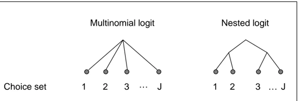
(16) assumption is violated due to transaction costs. For example, a rise in income may not lead to an immediate car transaction. The advantages and disadvantages of the different model categories with respect to forecasting vehicle ownership are discussed in Booz Allen & Hamilton (NZ) (2000). The main disadvantage of the aggregated models is that they omit many variables which affect car ownership at the household level. Nevertheless, these models have been found to perform reasonably well in short- to mediumterm forecasting. Disaggregated models, on the other hand, can include a number of explanatory variables at the household level. However, moving from the household to the regional or national level may lead to large errors at the aggregated level. Experience has also shown that disaggregated models tend to underestimate the growth in car ownership. The cohort model seems to overcome many of the problems in the other approaches. The only observed drawback is that these models are highly data-intensive.. 2.2. Car fleet composition. Vehicle type and age are important determinants for vehicle emissions. The future composition of the car fleet depends on the composition of new and scrapped vehicles. 2.2.1 Acquisition of new cars The composition of new cars is almost exclusively modelled on a disaggregated level, using models that describe household choices. The family of logit models has played an important role for modelling the choices of car type. The most frequently used models are the multinomial and nested logits. A schematic picture of the choice structure in these models is shown in Figure 2. The model equations and the link between logit models and the theory of random utility maximisation are described in Appendix I; see, for example, Cramer (1991) or Train (2002) for further details. In principle, a random utility function is attached to each possible state in a set of choices, and the outcome with the highest utility is chosen. The utility of a specific vehicle may depend on both the characteristics of the vehicle and the characteristics of the household or person.. Multinomial logit. Choice set. 1. 2. 3. …. Nested logit. J. 1. 2. 3 … J. Figure 2 Schematic picture of the multinomial and nested logit models with a choice set of J possible choices. The multinomial logit treats all choices the same way whereas the nested logit first groups choices into a number of nests. Both the multinomial and nested logits describe the choice between a finite number of discrete alternatives. In a multinomial logit, the odds of choosing one state over another are independent of all other alternatives in the choice set. This property is known as independence from irrelevant alternatives (IIA). If this. 12. VTI rapport 518A.

(17) property does not hold but the choice set can be grouped into subsets (also called nests) where the property holds within each subset, then the nested logit can be used. The multinomial logit has, for example, been used by Birkeland and JordalJørgensen (2001) to model the choice of car type. The choice set consisted of 50 alternative types. De Jong (1996) used a nested logit model to describe the choice of car type. The set of alternatives was divided into two nests, one with diesel and one with non-diesel cars. This division gave a significant improvement in the model fit as compared to a multinomial logit. Another application of the nested logit is presented in Mohammadian & Miller (2003). They used six nests, one for each class of car, and each nest comprised 4 classes of vintages. 2.2.2 Scrappage Both aggregated and disaggregated approaches have been used to model scrapping of cars. In aggregated models, the changes in cohorts of cars of specific ages are followed; sometimes the models also take into account car type. The changes in the cohorts are either described as the number of scrapped cars or as survival rates for cars of different ages. In the ALTRANS model (further described in 2.5.1), scrap page is modelled with a generalised linear model approach (Kveiborg, 1999). The number of scrapped cars of a specific fuel type, weight, and vintage is explained by a linear combination of variables such as price indices for fuel, repair costs, and income. An example of a disaggregated model of household behaviour is found in De Jong et al. (2001). They used a multinomial logit model to discriminate between five choices: keep, scrap, or sell for private owners, and keep or scrap for car dealers. The model was fitted to data from a stated preference (SP) survey of households that owned an old car (7 years or older) or had recently scrapped a car. These households received a questionnaire about intentions to scrap, intentions to replace and the relative importance of factors influencing these decisions.. 2.3. Car use. The modelling of car use has traditionally not received as much attention as modelling of car ownership (Wall, 1991). One explanation is, according to Wall, that the kilometrage per vehicle for a long time was relatively stable and it was more important to model car ownership. However, at least for Swedish conditions, Wall argues that the stability of kilometrage per vehicle was due to a balancing of factors that contributed to upward and downward trends. In the future, these factors may not balance each other and it is therefore important to pay attention to car use modelling as well. Wall (1991) used a log linear regression model to describe the average kilometrage per vehicle on an aggregated level. Average kilometrage was explained by fuel price, total private consumption, proportion of women car users, and proportion of pensioner car users. Regression models have also been used to explain car use on a disaggregated level. De Jong (1996) and Steg et al. (2001) used linear regression models to explain car use for a specific car and for a specific household, respectively. Golob et al. (1997) instead used a structural equation approach to model kilometrage given car type.. VTI rapport 518A. 13.

(18) 2.4. Licence holding. Although licence holding is not needed as input to emission models, it is highly relevant for modelling car ownership and use and is therefore included in this overview. Cohort models are often used to explain the development of licence holdings on an aggregated level. Applications can be found in HCG & TØI (1990), Byrsjö (1998), and Christensen & Gudmundsson (2003). Variables such as age, sex, and income are used to explain entry and exit propensities. On the disaggregated level, licence holdings have been modelled with discretechoice models. One example is the model described in HCG & TØI (1990) where the licence distribution within a two-adult household is described by a multinomial logit model. There are four choice alternatives: either the head of the household, the partner, both, or neither have a licence. Additional adults in the household are included in a separate model.. 2.5. Some specific model systems. Five different model systems are described in this section. The presentation of the systems includes only the parts that are relevant for this study, that is, the parts that pertain to car ownership, car use and the composition of the car fleet. The other parts of the models are described in the cited references. 2.5.1 The ALTRANS model ALTRANS is a transport model system developed by the National Environmental Research Institute in Denmark (Christensen & Gudmundsson, 2003). This system focuses mainly on public transportation, but car ownership and use are also included. The system is divided into three main parts. Part I: A GIS-based geographical model for travel times and distances. The model is based on detailed information of the public transport system such as timetables and routes. Distances by car can readily be calculated since the road structure is included in the model. Part II: A micro-economic model of individual travel behaviour. Mode choice, passenger kilometres travelled by each individual and each mode, and the number of cars possessed by each family are important outputs from this model. In addition, this part includes a sub-model of licence holdings. Part III: A car fleet and emission model. This model calculates the total emissions from the road and railway. Since the emissions differ for different types of cars and for cars of different ages, the composition of the car fleet is forecasted using a macro-economic approach. The cars are divided into 5 different types (3 sizes of petrol-driven cars and 2 sizes of diesel-driven cars) and 20 age classes. The number of cars owned by each family is estimated by a nested logit model with two nests. The nests divide the choices of having no car and having one or two cars (these are the only options). The variables used to explain the choices are: the costs of car ownership, socio-economic variables for the household and its individual members, accessibility of public transport, and number of licence 14. VTI rapport 518A.

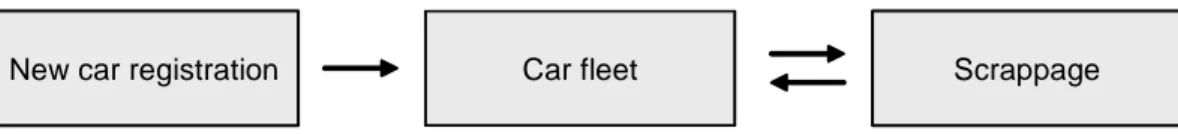
(19) holders. The sub-model of licence holdings operates on both the individual and the national levels. An individual’s probability of holding a licence is estimated by a binary logit model with the explanatory variables sex, age, income, occupation, and degree of urbanisation. These probabilities are used to assign licence holdings to individuals but also as inputs to a cohort model. The cohort model is used to forecast the number of licence holders on a national level, taking into consideration changes in the age structure and income. The model for the composition of the car fleet is based on the relation Stock(t) = Stock(t-1) + N(t) – Sc(t),. (1). where Stock(t) is the number of cars at time t, N(t) is the addition of new cars between time t-1 and time t, and Sc(t) is the number of scrapped cars during the same period. The size of the total stock of cars at different time points is provided from the travel behaviour model. The number of scrapped cars is calculated separately for cars of different types and ages; a linear regression model is used for each group of cars. The addition of new cars can now be calculated from (1). The new cars are distributed among the 5 types, and the distribution is assumed to be the same as for the base year of the forecasts. The total kilometrage of the car fleet is calculated in the travel behaviour model and distributed among different types and ages according to the following assumptions. First, all cars of the same age are driven the same distance, regardless of type. Second, the kilometrage differs between cars of different ages, but the relative kilometrage is constant in time. The distribution of driving distance for cars of different ages is calculated from surveys made at the Danish Road Directorate. 2.5.2 The COWI Cross-Country Car Choice Model The Danish consultancy group COWI A/S has developed a car choice model that can be modified to match the conditions of several different countries. The model was applied to Swedish conditions in a project that aimed at analysing the effect of introducing various CO2-differentiated registration taxes. Both the model and the study are described in Sand Jespersen et al. (2002). The model considers only the composition of the car fleet; use is not included. The main structure of the model is shown in Figure 3, and the three modules are described below.. New car registration. Car fleet. Scrappage. Figure 3 Basic model structure of the COWI Cross-Country Car Choice Model (from Sand Jespersen et al., 2002). The module for new car registrations includes a number of discrete choices made by the car buyers. The first choice is between a privately owned and a companyowned car, and this choice is decided by a binary logit model. The model input is the cost of having the car as a private car minus the cost of having the car as a company car. Given the choice of a privately owned car, a nested logit model describes the car buyer’s choice of car model. The nesting variable is car type (estate, hatchback, saloon, etc.). If a company-owned car is chosen, the buyer’s VTI rapport 518A. 15.

(20) decision is modelled with a multinomial logit. The buyer can be either the company or an employee depending on who makes the decision about car type. The models for both private and company cars take into account socio-economic conditions of the buyer and car characteristics, although the exact variables differ between the two models. The car choice models are disaggregated since they model the buyer’s choices. The scrapping module, on the other hand, consists of an aggregated model that estimates the survival rates of different car types and ages. The rates are based on both empirical survival curves for the Swedish car fleet and the effect that changed prices for new cars have on scrapping. These price elasticities are estimated on data from England and provided for three types of petrol-driven cars (based on engine sizes) and diesel-driven cars. The car fleet module uses outputs from the other two modules in order to keep track of the total car fleet. The composition of the car fleet in the base year is taken from the Swedish vehicle register. Each year the fleet is updated by the number of new cars and the number of scrapped cars. Used imported cars are not included in the model. In total, the car fleet is divided into 312 groups of cars, based on the following variables: − Age (0 to 25+) − Engine size (3 groups) − Fuel type (diesel and petrol) − Make (Swedish or not) 2.5.3 CARMOD CARMOD is a model system of the dynamics of the Australian car fleet, developed by the Bureau of Transport and Communications Economics. The model has been used to assess the effects of different measures on greenhouse gas emissions from the car fleet (BTCE, 1996). CARMOD is an aggregated model system that only considers the size of the car fleet as a function of time and total population. The number of vehicles per person at time t (MVPER(t)) is described by the following relation:. MVPER(t ) =. k 1 + ae −bt. (2). where k is the saturation level, and a and b are parameters that determine the shape of the curve. The parameters k, a, and b are estimated to fit data from the period 1945 to 1994. The system also includes a scrapping model with a structure similar to that of the model for vehicles per person. The proportion of cars of a specific vintage, i, surviving to an age of T years, Si(T) is modelled as S i (T ) =. 1 ai + (1 − ai )e biT. (3). where the size of the model parameters, ai and bi, depends of the vintage of the car. The results from the scrapping model are combined with the total number of vehicles per person and a forecast of the total population to provide a forecast of. 16. VTI rapport 518A.

(21) the total number of cars of different ages. The model does not include different car types. The average vehicle kilometres per car is assumed to be constant; however, the total kilometrage is distributed among vehicles of different ages according to the results from a survey of motor vehicle use. 2.5.4 FACTS (Forecasting Air pollution through Car Traffic Simulation) FACTS is a Dutch model that can be used to forecast car ownership, car use and emissions under alternative economic and demographic scenarios (De Jong et al., 2002). It is classified as a heuristic simulation method and based on two principal assumptions: a constant money budget and maintenance of mobility level. The assumption of a constant money budget implies that the percentage of income spent on travel is fixed for homogenous groups of households. In this case, households are grouped by age, income and composition. Maintenance of mobility level can, for example, have the effect that a household chooses to buy a cheaper car if the fuel price increases. The module in FACTS that describes car ownership and use is called SMAK and comprises the following steps. • Company cars are treated separately from private cars. These cars are allocated to households based on a probability distribution that is specific for each household group. • The available budget for private car ownership and private car use is determined. • The number of kilometres per household is determined by drawing from a specific probability distribution per household class. The household will be considered to own a car o if it has a mobility need above a predetermined minimum value, and o if it has a sufficiently large car budget. • If the above prerequisites are fulfilled, car ownership is determined based on the type of household, mobility needs, and whether the household has been allocated a company car. For example, a single household with a company car cannot own a private car. • The next step is to choose the car type. A total of 18 car types are distinguished based on the following variables: o Fuel type; 3 classes: petrol, diesel, LPG (Liquefied Petroleum Gas) o Weight; 3 classes: ≤ 950 kg, 951–1149 kg, ≥ 1150 kg o Age; 2 classes: ≤ 5 years old, > 5 years old The car choosing procedure involves several steps that will not be described here. In principle, the household chooses the most expensive car type it can afford (corrected for the number of kilometres driven).. The above steps are described in more detail in De Jong et al. (2002). This report also includes a discussion of the advantages and disadvantages of FACTS. One disadvantage is that the basic assumptions of a constant money budget for car ownership and use and maintenance of mobility level are at odds with economic theory.. VTI rapport 518A. 17.

(22) 2.5.5 DVTM (Dynamic Vehicle Transaction Model) A model system of car-holding duration, type choice, and use is described in De Jong (1996). All sub-models in the system operate on a disaggregated level. Car holding is described by a duration model which estimates the time between purchase of a car and its replacement. This model can be used to forecast whether a vehicle is replaced or not during a specific time period. Other transactions, such as acquisition and disposal, are not included, and only one car per household is considered. Given a replacement, the type choice is modelled by a nested logit model with separate nests for diesel and non-diesel cars. A total of 1,000 make/model/age-of-car combinations were included in the model, but each household could choose from a subset of 20 cars. The choices were influenced by the following factors: − income and cost variables, − comparison of previous and new car attributes (to account for such things as brand loyalty), − attributes of alternatives on the car market.. Car use is described by the following regression model:. ln(k i ) = α ln( y i − ci ) + βvi + γZ i + ei. (4). where i indicates the decision-maker, ki is annual kilometrage in the car, yi is annual net household income, ci is fixed car costs, vi is variable car costs, Zi is a vector of attributes of the decision-maker, ei is the error term, and α, β, γ are model parameters.. 2.6. Factors included in existing models. An overview of variables used to explain car ownership, car type, and car use on the aggregated and disaggregated level is presented in Table 1 and Table 2, respectively. The list is far from exhaustive, but it covers the principal variable types. Most models use variables listed in the tables or closely related variables. The trends in aggregated time series data are typically explained by demographic and macro-economic factors. When household behaviour is modelled, the most commonly used variables are socio-demographic and socio-economic household data and car characteristics and costs. In addition to the variables listed in Table 1 and Table 2, motivational factors have been considered in a couple of studies. Steg et al. (2001) included a variable that described environmental awareness when modelling car use. Wu et al. (1999) emphasized the importance of including psychological and sociological factors when modelling car ownership in developing countries. They included use-value attitudes and sign-value attitudes in a model of car ownership in China.. 18. VTI rapport 518A.

(23) Table 1 Overview of variables used in aggregated models of car ownership, car type, and use. Variable type. Examples of variables. Demographic. Population size Proportion of inhabitants in different age groups Proportion of cars owned by pensioners Proportion of cars owned by women Number of licence holders. Macro-economic. Gross domestic product (GDP) Consumer price index Fuel price index Total private consumption index Income index Purchase price index. Table 2 Overview of variables used in disaggregated models of car ownership, car type, and use. Variables related to. Variable type. Examples of variables. Household. Socio-demographic. Size of household Number of children Age Gender Living area, urban or rural Housing form Income Employment status Education level Number of licence holders Service station availability (relevant for alternative fuel cars). Socio-economic. Other. Household vehicle fleet. Car. Number of owned cars Average market price of household fleet Average age of household fleet Fixed costs. Variable costs Car characteristics. VTI rapport 518A. Purchase price Annual vehicle tax Insurance Operating costs Fuel price Operating costs Engine size Fuel-type Age Other characteristics such as van, sports car, or SUV Brand Model. 19.

(24) 3. Gaps and shortcomings in existing model systems. The orientation of existing models in the previous section showed the wide range of models that have been applied in the area. A lot of effort has been spent on elaborating the causes of household choices and overall trends. However, it is not as simple as copying an existing model system. This conclusion is based on two observations. First, none of the studied systems are complete with respect to our requirements of a new system described in the introduction. Second, the disaggregated choice models generally exclude important factors that affect the choice process, such as attitudes and preferences.. 3.1. Limitations of the model systems. The five model systems described in section 2.5 all have shortcomings in relation to the requirements of the new model system. The main limitations of each system are described below. The ALTRANS model The disaggregated car ownership model in ALTRANS is static whereas the general recommendation in the recent literature is to use a dynamic model (see section 2.1). Moreover, the system does not include an explicit car type choice model; the distribution of new cars is assumed to be the same as for the base year of the forecasts. Thus, changes in household characteristics do not lead to changes in composition of the car fleet. Another limitation is that all cars of the same age are assumed to be driven the same distance, regardless of type. The COWI Cross-Country Car Choice Model The COWI model also includes a static ownership model. The use of the car fleet is not included in the system. CARMOD This system differs from the first two since it only operates on an aggregated level, thus, household behaviour is not modelled. The total number of cars depends only on total population and time, which limits the use of the model as a scenario explorer. Car types are not included. FACTS (Forecasting Air pollution through Car Traffic Simulation) The limitations of FACTS are thoroughly discussed in De Jong et al. (2002). A couple of the main objections are mentioned here. As in the ALTRANS and the COWI models, FACTS uses a static car ownership model. Moreover, the two basic model assumptions, constant money budget for car ownership and use and maintenance of mobility level, are at odds with economic theory. Finally, the choice of car type is influenced only by car cost (not by other attributes of the household). DVTM (Dynamic Vehicle Transaction Model) DVTM, as described by De Jong (1996), only included replacements of cars; no other transactions, such as acquisitions and disposals, were included, which, of course, severely limited the use of the model. Since 1996, those other transactions. 20. VTI rapport 518A.

(25) have been introduced, according to De Jong et al. (2002). To our knowledge, the extended model has not been published and we can therefore not evaluate the merits of these improvements. The five systems briefly described in this report have been chosen to show the diversity of operational systems. A number of other systems also exist, but we have not been able to find any other system that fully matches our requirements.. 3.2. Absence of motivational factors. Most of the disaggregated models take into account socio-economic and sociodemographic factors that are easily observed (Choo & Mokhtarian, 2004). However, the models cannot explain why two neighbours with the same socioeconomic and socio-demographic status own completely different types of cars, or why one neighbour takes the car and the other takes the bus to work. The underlying motivations that lead to these differences in behaviour are difficult to measure but nonetheless important to understand for three main reasons. First, the lack of important explanatory variables may lead to model misspecification and, consequently, errors in the resulting parameter estimates. Second, forecasting the response in model outputs due to changes in motivational factors could be important in scenario calculations. Third, understanding the motivational factors is the key to changing undesirable behaviour. The problem of model misspecification can for some cases be solved by using a flexible model specification (Train, 2002). A flexible model structure may, however, lead to other problems such as overparametrisation. A few papers acknowledge the importance of including motivational factors in the models, as mentioned in section 2.6. Steg et al. (2001) report from a literature study which revealed that factors such as emotions evoked by car use, social norms, personal norms, and awareness of the problems caused by car use were related to car use and travel mode choice. Kitamura et al. (1997) found that attitudinal variables were more important than socio-economic and neighbourhood descriptors for explaining trip frequency of different modes. However, their results were based on a study with very low response rate (17.6%), so the merits of these results are highly questionable.. VTI rapport 518A. 21.

(26) 4. Purchase behaviour and the decision process. The experiences of including motivational factors in car ownership models are very limited. We have therefore studied the literature of car purchasing behaviour and the decision process. For understanding the behaviour involved in purchasing an item, the theory of planned behaviour can be used, according to Caprara et al. (1998). This is a model that predicts a person’s behaviour via one’s intention to engage in that behaviour. The intention is predicted by three parameters: attitude towards the behaviour; subjective norm, which means the person’s perception of the social pressure to engage in the behaviour; and perceived behavioural control, which means the person’s perception of how difficult or easy it would be to perform the behaviour (Figure 4). Behavioural Beliefs. Attitude. Normative Beliefs. Subjective Norm. Control Beliefs. Intention. Perceived Behavioural Control. Past behaviour. Figure 4 Theory of planned behaviour.. These three predictors are functions of other variables. Attitude is a product of a person’s behavioural beliefs, that is, the perceived consequences of the behaviour. Subjective norm is a product of normative beliefs, which means perception of other important persons’ preferences about whether one should engage in the behaviour and one’s motivation to comply with those preferences. Perceived behavioural control is determined by control beliefs, that is, the subjective probability that a certain event should occur and whether this would facilitate or hinder the intended behaviour. When looking at consumer behaviour there has been an addition to the model, which is past behaviour. This parameter will measure self-reported habits and could, for example, explain brand loyalty. When purchase intention of a car (an Opel) was tested with this model, it was shown that the parameter attitude was most important to discriminate between users and non-users and the main difference among the two groups regarded behavioural beliefs, that is, those issues that are considered as possible outcomes of the behaviour. There was also a difference in normative beliefs. More specifically, this result showed that users believed more than non-users that the purchase of an Opel would have outcomes such as strong, durable car without problems, reliable car, providing safety, high-level of comfort and good qualitycost relationship. The users also believed that their relatives (children, partner etc.) would like it and they were more inclined to comply with their approval. They also believed that the purchase would be facilitated by a good price. 22. VTI rapport 518A.

(27) Taken together it was attitude towards purchasing the Opel and past behaviour that were the best predictors of the purchasing intention. Perceived control and subjective norm were less relevant even if these also were significant (Caprara et al., 1998). Choo & Mokhtarian (2004) suggested other factors that affect purchase behaviour. They found that travel attitudes, personality, lifestyle and mobility significantly affected an individual’s vehicle type choice. Attitudes can also affect mode choice. Car users often have positive attitudes towards car use and do not see the negative effects. The feeling of freedom is stronger than the concern of greenhouse gas emissions. Why should I sacrifice for the collective interest when others do not? Why shouldn’t I take the car when everyone else do? Discussions like this make car users continue to use their cars (Golob & Hensher, 1998; Tertoolen et al., 1998). This positive attitude towards driving leads to a frequent use of the car and there is no reflection of whether it is good to use the car or not (Boe et al., 1999). Literature about factors affecting purchase behaviour is limited; there is more about the decision process to purchase a car. Marell et al. (1996) have studied the decision process that leads to replacement. They found that there are a lot of models with information about factors affecting the choice of which type of car to buy but there is almost no information about the decision-making process leading up to the purchase. Every car owner has an aspiration level defining a minimal acceptable quality standard for the car. The car owner also has a current level, which means that they judge the current quality of the owned car. If there is a discrepancy and the discrepancy is strong enough between those two levels, it will lead to replacement. Several factors affect the aspiration and current level such as economy, taste marketing and other socio-demographic factors, but the relation among those aspects has to be investigated further (Marell et al., 1996; Punj & Brookes, 2002). When the car owner has decided to replace the car he/she starts seeking information about model, size, engine etc., but often this is not the starting point. The decision to replace a car consists of several “sub-decisions”. Some of these sub-decisions have already been made in advance, before the decision of replacement is made. A lot of consumers make product-related decisions in advance and store them in memory for later use; such stored decisions are called pre-decisional constraints. These pre-decisional constraints could be either marketer-related or household-related. Marketer-related refers, for example, to brand choice (Saab or Volvo) or which dealer to go to. The consumer could, for example, have decided that the next time he or she buys a car it will be a Volvo. Household-related constraints are not brand-dependent; it is more about the price of the car or the size, etc. These pre-decisional constraints influence the rest of the decision process and the information search, but the nature of their influence depends on why the current vehicle is being replaced and on the circumstances at the time. It seems like consumers with marketer-related pre-decisional constraints simplify their purchase decisions more than those consumers with householdrelated constraints. The first group may decide which car to buy at the same time as they decide to replace the car. Those with household-related pre-decisional constraints seem to make a more complex and engaging search with more considerations. This shows a bit of the internal dynamics of the consumer decision process and different processing strategies (which sometimes seems to simplify the decision, and sometimes does not). VTI rapport 518A. 23.

(28) When it comes to searching for information, the individual’s beliefs, earlier experience and cognitive abilities have a role. According to TRB (1996), the purchaser’s motivation (which is influenced by his or her beliefs and experiences) shapes how much effort goes into collecting information and where the information is sought. The information is plentiful and available from many different sources, and sometimes it is difficult to get the right information. If the product is expensive and important there is greater interest in getting information, and cars seem to be important. Consumers’ cognitive abilities are varied, and therefore they search for, transform and use information in very different ways and so different purchasers will make different decisions. Their memory, knowledge and beliefs are different. People use new information in their existing beliefs. If they know nothing about the topic it could be hard to understand or it could be misunderstood. Buying a car can be complex since there are numerous alternatives, and therefore many people eliminate a lot of alternatives and thereby minimize complex and difficult calculations and trade-offs. It is therefore important to consider how the information is framed and presented because that affects how it is perceived. Whether the available information is deemed good enough and worth paying attention to depends on internal factors, that is, if it is perceived that the information will help in meeting desired goals and if it is consistent with the individual’s prior beliefs. It also depends on external factors, such as the design, density and clarity of the information, for example. Another factor that affects the decision process could have to do with personality and is called cognitive closure. Houghton & Grewal (2000) observed that different people need and want to have different kinds of information. Some people want to come to cognitive closure quickly, which means that they want a firm answer to a question and do not want ambiguity. This type of person and consumer will make a quick decision on few pieces of information, and he or she will avoid information that is incongruent with previously formed beliefs because that type of information could reopen the closed decision process. This means that people with a high need for cognitive closure who also have a brand preference are likely to maintain a positive image of the brand as they are unlikely to search for an alternative. They would also avoid and ignore negative information about the brand, as this information would frustrate closure. This would lead to a focus on information with stereotypical evidence instead of diagnostic evidence. So people with a high need for cognitive closure do not search for information as much as people with a low need for cognitive closure (Houghton & Grewal, 2000). The conclusion of this section is that there are a number of factors other than socio-economic and socio-demographic ones that affect consumers’ decision process in buying a new car. Some of them have been presented here, but there are others. So even if the neighbours look the same from the outside, they have different beliefs, experiences, attitudes etc., and they handle the decision process in different ways due to these factors. But how these factors relate to each other and what weight they have in the decision must be further analysed.. 24. VTI rapport 518A.

(29) 5. A proposition of a new model system. In section 3, we concluded that none of the described model systems fully comply with our requirements as described in the introduction of this report. A new model system is therefore proposed. The formulation of the system is based on experiences and ideas from existing models described in section 2. The national model system for analysis of passenger transport, Sampers, describes how people choose to travel. Important outputs are travel frequency, destination choice, travelling time, and choice of transport mode. The system also includes a car ownership model developed at VTI. It is, for specific applications, important that the new system provides forecasts that are consistent with the forecasts from Sampers. It will therefore be possible to run the new model both with and without Sampers co-ordination. An improved car ownership model could also replace the one included in the current Sampers version.. 5.1. Overview. The proposed model system operates on two levels: the aggregated (national or regional) level and the disaggregated (household or personal) level (Figure 5). Forecasts of the total number of cars and total kilometrage are provided from the aggregated models whereas the disaggregated models provide the distribution of cars of different types and ages and the distribution of kilometrage over the same classification of cars. These results are then combined to give the final outcomes, the number and kilometrage of cars of different types and ages. Aggregated level. Car ownership (1). Licence holdings (3). Total number of cars Total kilometrage. Total kilometrage (2). Disaggregated level. Licence holdings Household car transactions (4). Kilometrage per car (5). Combination of outputs from the aggregated and disaggregated models with total number of households of different categories (6). Composition and use of each household car fleet. Total number of cars of different types and ages Total kilometrage of cars of different types and ages. Model Outputs. Figure 5 Overview of the proposed model system. The boxes with unbroken lines indicate models, and boxes with dashed lines indicate model outputs.. The main idea behind the two-level system is to overcome the disadvantages that are linked to each type of model category. The disaggregated models have been. VTI rapport 518A. 25.

(30) shown to underestimate the growth in car ownership (Booz Allen & Hamilton (NZ), 2000). This observation is primarily based on static models that do not capture the long-term trend of increasing car ownership. The problem should be less pronounced for dynamic transactions models, but, since they are often adjusted to short time-series, there is a great risk that they also will underestimate ownership growth. Furthermore, small errors at the household level can add up to large errors at the national or regional level. An aggregated car ownership model is therefore used to control the level of the total number of cars. The strength of the disaggregated models is that they take into account variables that affect decisions at the household level and thereby contribute to the understanding of household behaviour. Car transactions and car type choices are therefore modelled at the disaggregated level. The same reasoning applies to car use. Total kilometrage of all cars is estimated at the aggregated level. The kilometrage of a specific car is assumed to depend on both characteristics of the car and the car owner and is therefore modelled at the disaggregated level. The two-level system also enables efficient use of data since different data sources can be used for different levels. For example, aggregated models can be based on individual-based registers such as the Swedish vehicle register while disaggregated models can be based on household surveys. A similar model approach has been used in Australia. The overall level of car ownership was described by an aggregated model, and the cars were then distributed within urban areas using disaggregated models (see Grouenhout & Bell, 1985; RCA & Travers Morgan, 1981; Travers Morgan, 1982; all cited in Booz Allen & Hamilton (NZ), 2000). 5.1.1 Basic concepts Car types The basic constraint is that the classification of car types should be consistent with the classification used in the ARTEMIS model. The list of car types in ARTEMIS is not finalised so a definite classification cannot yet be made. What we do know is that petrol and diesel cars, each divided into three classes of cubic capacity, will be included. Alternative fuel type cars will also be included, but the exact categories are not determined. In addition to the above categories, we will also distinguish between cars of different sizes/functions since this may be important for household choices. A large car with a relatively small engine or a small car with a large engine may be similar with respect to emissions but appeal to different types of households. To start with, we will adopt the classification that Euro NCAP uses when they present their results of crashworthiness: super minis, small family cars, large family cars, executive cars, small MPVs, large MPVs, small off-roaders, large off-roaders, and roadsters. Depending on the composition of the Swedish car fleet, we may need to merge some classes in order to achieve a sufficiently large number of cars in each class. In summary, the model will distinguish car types defined by the following variables, although not all combinations of these variables will exist: − Fuel type (at least 3 classes) − Cubic Capacity (3 classes) − Size/functions (9 classes).. 26. VTI rapport 518A.

(31) Households The majority of the disaggregated models in the literature are household based, that is, the decisions are assumed to be made by the household as a unit. The household concept is rarely defined, but the following definition, frequently used by Statistics Sweden (SCB), is probably generally applicable; this definition says that persons who live in the same dwelling and who share the housekeeping belong to the same household. This definition is, however, impractical to use since such households cannot be identified in the Swedish national registration of the population. Only the more restricted family can be identified; a family consists of a married couple with or without children, and unmarried couple with children under the age of 18, or a single person with or without children. Unmarried couples without children are defined as singles. Since forecasts of the population also are restricted to families, the disaggregated models in the proposed model system will be based on families instead of households. Hereafter, the words will be used synonymously. Model time steps The model will operate on an annual time step. State variables such as the number of cars a household owns will be evaluated at the end of each year whereas kilometrage will represent the total distance driven throughout the year. Motivational factors The term motivational factors is here used in a wide sense to cover factors such as attitudes, norms, and preferences. The conclusion from section 4 was that further research is needed before we can point out the most important factors to include in the model system. For now we will only describe where the motivational factors are important to consider. Privately owned and company-owned cars Both privately owned and company-owned cars that are available for private driving are handled in the system. Company-owned cars that are strictly used for business purposes will not be included at this stage. 5.1.2 Co-ordination with Sampers Forecasts of the total number of cars and total kilometrage from Sampers are used as a basis for national and regional transportation planning by the Swedish Road Administration (SRA) and the Swedish Institute for Transport and Communications Analysis (SIKA). Emission rates are often calculated as complements to these outputs. It is important for the credibility of these applications that the emission calculations are based on data that are consistent with the forecasts from Sampers. Co-ordination with the Sampers system could also improve the quality of our forecasts since that system also includes other transportation modes. It is, on the other hand, also valuable to have a system that works independently of other systems. To meet both standpoints, it will be possible to run the system both with and without Sampers co-ordination. Three different modes are suggested: coordination at the aggregated level (mode 1), co-ordination at both the aggregated and disaggregated levels (mode 2), and independent mode (mode 3). The coordination affects three of the sub-models, number (1), (2), and (5) in Figure 5.. VTI rapport 518A. 27.

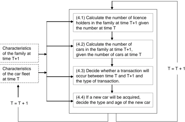
(32) The implications of the different modes are explained in relation to the summary of these sub-models in the next section. 5.1.3 Summary of the sub-models This section includes a brief summary of each sub-model, and a more detailed description is provided in the next section. The model number corresponds to the numbers in Figure 5.. Car ownership (1) Car ownership at the aggregated level is described by a cohort model. The model is essentially the same as the one developed at VTI (Matstoms, 2002), which is also included in Sampers. Here, we suggest an improvement of the model by entering, for example, licence holdings as an explanatory variable. The version of the model currently implemented in Sampers will be used in the co-ordination modes. Total kilometrage (2) Total car kilometrage from Sampers is used here if the model is run in either of the co-ordination modes. In the independent mode, total kilometrage is estimated in two steps. First, the average number of kilometres per car is calculated by a log-linear regression model following the ideas from Wall (1991). Second, the total kilometrage is obtained by multiplying the average car kilometrage by the total number of cars provided from sub-model (1). Licence holdings (3) Aggregated licence holdings are, like car ownership, described with a cohort model. Licence holdings are included only to provide inputs to the car ownership model (1) and are therefore used only when the system is run in the independent mode. Household car transactions (4) This sub-model is the most comprehensive part of the model system. It is a dynamic transaction model describing household behaviour. Dynamic models are generally recognised as superior to static models when it comes to describing a household’s car purchasing behaviour (Kitamura & De Jong, 1992; Ramjerdi et al., 2000). The main reason is that static models are based on the assumption that households are constantly in equilibrium with respect to their car fleet. This assumption is violated due to the costs involved in buying a new car. A transaction model can either estimate the duration between transactions (duration models) or whether or not a transaction has occurred during a specific time interval (discrete-time models). There is no clear preference for either of the models in the literature. Kitamura & De Jong (1992) proposed a discrete-time frequency model rather than a duration model. However, their main motivation for this was that the duration models did not take into account time-varying explanatory variables. This limitation has been overcome in later versions of these models, so that reason for proposing a discrete-time model no longer holds.. 28. VTI rapport 518A.

(33) Nevertheless, the report by Kitamura & De Jong (1992) is valuable since it describes how the transaction models can be linked to economic theory. We will apply a discrete-time model. This way, we only need to know whether or not the household has changed its car fleet from time T to time T+1; we do not need to know how long a household has owned a specific car. The number of cars per household at the end of each year is described with a Markov chain model. Whether a transaction has occurred and the type of transaction are modelled given the results from the Markov model. The following transactions are possible: purchasing an additional car, replacement, and disposal. If a car is disposed of, it can either be sold or scrapped. If the household buys a new car, the car type and age are determined in a separate model. This sub-model is not influenced by Sampers co-ordination, and the same version of the model is used in all modes. Kilometrage per car (5) A modified version of the regression model in DVTM will be used to estimate the annual kilometrage of a specific car type (De Jong, 1996). The kilometrage is explained by characteristics of both the car and the household. Results from the regression models are combined with outputs from Sampers if the system is run in co-ordination mode 2. Sampers gives total car use per person but the kilometrage is not linked to a specific car type. The total kilometrage for a household calculated by Sampers will therefore be distributed between the household cars according to the results from the regression model. Combining aggregated and disaggregated results (6) The results from the aggregated and disaggregated models are here combined to provide the final outputs from the model system, that is, total number of cars of different types and ages and total kilometrage for the same division of cars. The calculations include sample enumeration of the household outcomes.. 5.2. Description of the sub-models. This section includes descriptions of all six sub-models of the forecasting system. The version of the system described here is the version that can be run independently of the Sampers system. 5.2.1 Car ownership (1) VTI has developed a regional car ownership model (Matstoms, 2002) which was completed in 1999. This model can provide forecasts on both the national and municipal levels. Although it is an independent model, today it is primarily used as an integrated part of the Sampers system (Beser & Algers, 2001). The model relies on estimates of individuals’ entry and exit propensities to and from car ownership. This refers to the proportion of the population that had no car but acquired one during a given year, and, conversely, to those who gave up car ownership status during that time. Non-linear regression models for the entry and exit propensities were estimated on rich statistical material, covering all adults in Sweden and their car ownership status 1980–1995. The most important variables are the individual’s age, sex and region of residence. Besides these variables, the models also depend on income, petrol price, increase of GNP, and the proportion of leased-out cars. The last variable is included in order to incorporate company-. VTI rapport 518A. 29.

(34) owned cars in the model. The model equations are described in detail in Matstoms (2002). As a part of the proposed model system, we suggest that the model will be improved by including licence holdings as an additional explanatory variable. The total number of licence holders in different groups classified by age and sex will be provided from the licence-holdings model (3). The geographical dimension is handled in the following way. The almost 300 municipalities in Sweden are divided into a certain number of homogenous groups, and for each group the model is estimated separately. That means that all models have the same basic form, but municipalities in different groups have different coefficients. Given the above types of models, the future number of car owners, by age, sex and municipality, can easily be expressed by a simple recursive relation. A detailed description of the number of car owners the first year and a corresponding description of the population for all coming years are then assumed. 5.2.2 Total kilometrage (2) Total kilometrage is calculated as the average number of kilometres per car times the total number of cars. The average number of kilometres per car is described by a log-linear regression model following the ideas from Wall (1991). The general form of the model is. ln Y = ln β 0 + β1 ln X 1 + β 2 ln X 2 + ... + β P ln X P + ln ε. (5). where Y is the dependent variable, X1, ..., XP are explanatory variables, β0, β1, ..., βP are regression parameters and ε is an error term. The parameters can be estimated with ordinary least squares methods. Edwards et al. (1999) have developed a model for calculating the total kilometrage of different types of vehicles in Sweden (motorcycles, cars and light trucks, heavy trucks, etc). Total kilometrage for each year from 1950 onwards have been calculated with this model. These data, divided by the total number of cars will be used as the dependent variable. The choice of explanatory variables very much follows what Wall (1991) suggested, but we have made some modifications to comply with the data that are available from official sources. The basic set of variables will be fuel price index, income index, number of cars per 1000 inhabitants, proportion of cars that are owned by pensioners, and proportion of cars that are owned by women. The resulting set of variables that will be included in the model will be a result from the model development. A couple of potential problems with this model approach were highlighted in Wall (1991). First, he experienced some problems with the parameter estimation, due to multi collinearity in the explanatory variables. However, since we will not use the exact variables he did, it is not possible to say beforehand whether the same problem will occur. If it does, we can either modify the model specification or use another estimation technique. The second problem was that the residuals followed a pattern that is typical for positively auto correlated data. If this is the case, the parameter estimates may be biased. Again, we do not know if this will occur in our model, but if it does, it can be handled by modelling the errors in (5) as an ARMA process; see for example Makridakis et al. (1998).. 30. VTI rapport 518A.

No results found