Automatic temperature monitoring of brakes on heavy vechicles

VT1 notat

Number 354A-1994 Published 1994

Title: - Automatic temperature monitoring of brakes on heavy vehicles

Author: Göran Edvell

Group: Environment

Project code: 20028

Project: Automatic temperature monitoring of brakes on heavy vehicles

Financed by: The Swedish Communications Research Board (KFB) Distribution: Free div Väg- och transport-forskningsinstitutet ä

Automatic temperature monitoring of brakes on heavy vehicles Göran Edvell

PREFACE

This Master of Science Thesis in Applied Physics and Electrical Engineering at Linköping University of Technology was carried out at the Swedish Road and Transport Research Institute (VTI) in Linköping. It is the first phase in the project Automatic temperature monitoring of brakes on heavy vehicles . The contractor was The Swedish Communications Research Board (KFB). The thesis is in the

subject of Measurement technique at the IFM, Institution of Physics and

Measurement Technique, Linköping University of Technology (LiTH).

Special thanks to my supervisor, Lars-Gunnar Stadler (VTI), for his help and encouragement and for putting up with my somewhat odd working hours.

Many thanks to my examinator, Bengt Sandell, director of studies, for his comments and viewpoints on the report, being the supervisor of the theoretical part of the report.

Furthermore, I would like to thank the following persons for their support:

Wolfgang Schurig, Cooper Tools, providing the iron-nickel magnastats mounted in the brake disc,

Siegfried Höfler and Alf Wiklander, WABCO, supplying the two ABS sensors used for detecting the magnetic state of the magnastats,

Bo Sundman, KTH, and Johan Carlsson, LiTH, giving a hand with the THERMOCALC program,

Patric Johansson, the Institute for metal research in Stockholm, for his views on the manufacture of magnetic materials,

Olof Jacobsson, VOLVO Car Corporation, who helped me with the measurements in Gothenburg and who together with Mats Fagergren, VOLVO Truck corporation, facilitated the use of the test .laboratory for brakes at VOLVO,

Per Rundbom, Vactek for the test material and Ann-Sofie Senneberg (VTI) who edited the text. Christina Ruthger for the translation into English.

Finally, many thanks to all those who contributed to this examination work and made it a positive experience.

Göran Edvell, Linköping, 1994-03-24

CONTENTS

PREFACE

ABSTRACT

1.1 Background

1.2 Aim

1.3 Scope

1.4 Method

1.5 Criticism of the method and sources

2 THEORY OF MAGNETlSM

3 MAGNETIC MATERlALS

3.7 Suitable materials

4 MEASUREMENT METHOD

4.1 Measurement principle 4.2 Detection of magnetic material

VTI Notat 35A-1994

10 12 13

17

4.3 Advantages and disadvantages of the method

5 TEST EQUIPMENT

6 MEASUREMENTS

7 SUMMARY AND DISCUSSION

REFERENCES

Appendices 1-5

VTI Notat 35A- 1994

18

19

30

33

35

ABSTRACT

This report describes a feasibility study of the possibility of measuring the temperature of vehicle brakes by means of the Curie-Weiss effect, i.e. the loss of magnetism in a ferromagnetic material when a speciñc temperature, the Curie temperature, is exceeded. By monitoring the magnetic state of the material, it can be decided whether the temperature is above or below the Curie temperature. The method is planned to be used in automatic brake control systems. The study contains theory and experimental work.

A theoretical study of suitable ferromagnetic materials shows that the alloys Cu-Ni and Co-Cu-Ni have Curie temperatures that can be varied between O°C and 950°C without causing any structural changes in the alloys.

The design of the measuring equipment and the construction of the necessary electronics for measuring the temperature of a brake disc are described. The measurements show that for the ferromagnetic materials used in the tests, the state transition interval from non-magnetic to magnetic state is at most 15°C. This is regarded as sufñciently small for the method to be suitable for use in a brake monitoring system.

1

INTRODUCTION

1.1 Background

Accidents caused by defective brake systems on heavy vehicles may have disastrous consequences. In one accident at Måbødal in Norway in 1988, twelve

pupils and three adults were killed on a school trip when the brakes of their bus

failed. A bus accident on the coast of Tarragona (Spain) where 180 persons were killed is another example.

Investigations carried out by the German organisation DEKRA show that 47.9% of all accidents due to technical faults are caused by defective brake systems. As a

comparison, the TUV (Technische Uberwachungs Verein) statistics report 59%

[8:23].

An adequate brake monitoring system is thus very important from a traffic safety point of view. By monitoring the temperature process in brakes, functional faults and fading can be detected [8].

Measuring the temperature in vehicle brakes is, however, difficult. The main reason is the environment with vibrations, high temperatures, dirt and corrosive attack. As the brake disc or drum rotates, contactless measurement is preferred. The conventional techniques currently used for measuring temperature in vehicle brakes are designed for laboratory environment or occasional field tests [4].

Despite the need, there is no commercially available system for continuous temperature monitoring of vehicle brakes. Such a system would be of great value. Examples are a system for the thermal protection of brakes and a system for monitoring temperature processes in brake systems. Tests with thermal elements and infrared optical pyrometry have been carried out by Lucas Automotive GmbH in Germany [8].

Lars-Gunnar Stadler of the Swedish Road and Transport Research Institute (VTI) has suggested a new principle for measuring temperature in vehicle brakes.The method is based on the Curie-Weiss effect, whereby magnetic materials become non-magnetic when the Curie temperature is exceeded. The advantage of the method is that it is very robust and thus able to cope with the unfavourable

measuring environment in vehicle brakes. Furthermore, it requires no calibration

or contact and is simple to use.

1.2 Aim

It is of interest to study whether there is any practical method of monitoring the temperature in vehicle brakes. In this case, the problem is formulated as follows: 0 Is the method of measuring temperature with the Curie-Weiss effect suitable

for continuous measurement of temperature in vehicle brakes? 0 What are the physical limitations?

0 Is the method practicable?

The aim of the thesis is to try to answer these questions, i.e. to analyse the physical limitations of the method and to design a working temperature indicator, based on the principle mentioned above.

1.3 Scope

Not all magnetic materials that can theoretically be used in the measuring method, were studied. Only a limited number of materials were chosen. The choice was based on judgements of the suitability of each material concerning the Curie temperature, melting point, corrosion resistance and other Characteristics of the

material. Some materials were also sorted out from this sample as the number of ferromagnetic materials is relatively large.

The aim of the thesis is not to produce a commercially marketable product. Instead, it must be seen as phase one in a large project where phase two aims at producing a finished product if phase one is successful. The aim of the first phase of the project is to show that temperature can be measured with the above-mentioned technique.

Only one alternative of measuring temperature with the Curie-Weiss effect was studied owing to insufficient time and resources for studying other methods. One such method could have beenthe use of a sensor based on the Hall effect.

1.4 Method

The work was divided into two parts:

0 a theoretical part, where suitable magnetic materials were studied,

0 a practical part, where an instrument for measuring temperature was

constructed and tested.

The theoretical part is mainly based on literature studies, as well as on verbal information from researchers in the areas in question.

The practical part comprised the construction of measuring equipment. Lars-Gunnar Stadler was responsible for the mechanical construction while the author developed the necessary electronics.

The measuring equipment was then tested in the test laboratory at VOLVO Car Corporation in Gothenburg. The tests were accurately documented and the test

results were evaluated at the Swedish Road and Transport Research Institute in Linköping.

1.5 Criticism of the method and sources

It cannot, of course, be guaranteed that the method of measuring temperatures in vehicle brakes with the Curie-Weiss effect has never been tested, but as the technique is unknown to VOLVO, SAAB, WABCO and Lucas Automotive, according to the author's experience, this is probably the first time it has been tested. Unfortunately, samples of the magnetic materials copper-nickel and cobalt-nickel, discussed in Chapter 3.7, could not be made or tested owing to insufñcient

financial resources.

The Curie temperatures for the magnastats of nickel-iron, used in the practical tests, were not checked as the equipment for such tests was not avialable. The Curie temperature of the magnastats stated by the manufacturer was assumed to be reliable.

2

THEORY OF MAGNETISM

A magnet attracts a piece of iron even if the two are not in contact. The interaction of forces between the two bodies is caused by a magnetic field designed H (A/m). A magnetic field can be produced by both an electric current and a magnet. The magnetic field has a direction and a size, i.e. it can be described as a vector.

In order to describe the magnetic Characteristics of a material, a quantitative measure for magnetisation has to be defined. This can be done by a magnetic dipole moment per unit volume designed M (Alm) and defined according to the following formula [3224],

nAv

_ . k=1 .

M - Av (equation 2.1)

where Av is volume and mk (Amz) is the magnetic dipole moment for an atom caused by the rotation of the electrons around the atomic nucleus on the one hand and the rotation of the nucleus around its own axis on the other hand. The magnetic dipole moment caused by the nucleus is usually insigniñcant in relation to the moment caused by the electrons. The magnetic dipole moment of the atoms in equation 2.1 must be added as vectors, thereby obtaining both direction and length. A knowledge of quantum mechanics is, however, necessary to fully understand the magnetic properties.

If a material is placed in a magnetic field H, the magnetisation M of the material is changed according to

M = Xm * H (equation 2.2)

where Xm is the magnetic susceptibility. For some materials, Xm depends on the added field H.

Faraday showed that some magnetic properties can be compared with a flux. The flux lines pass from a magnetic material out in the air at the magnetic north pole, enter at the south pole and pass through the material from the south pole to the north pole to form a closed loop.

The total number of flux lines crossing an area at right angles is called the magnetic flux (I). Magnetic flux per unit area is called magnetic flux density and is designated B (T). Both H and M contribute to the magnetic flux density. The relationship between B, H and M is

B = pg (1 + Xm) H = ;10 nr H = uH (equation 2.3)

;.10 = 41: * 10'7 (Vs/Am)

(equation 2.4)

Sometimes, the term permeability, ur, is used instead of magnetic susceptibility. The relationship between magnetic susceptibility and relative permeability is

M = 1 + Xnn (equation 2.5)

The constant ;10 is the permeability in vacuum and u is called the absolute permeability or sometimes only permeability.

3

MAGNETIC MATERIALS

3.1 Introduction

All materials can be divided into three classes depending on their magnetic susceptibility. A material is said to be

diamagnetic, if Xm<0, i.e. a small negative figure, e.g. copper, paramagnetic, if Xm > 0, i.e. a small positive figure, e.g. aluminium, ferromagnetic, if Xm is a large positive figure, e.g. soft iron.

Diamagnetic and paramagnetic materials are non-magnetic , while ferromagnetic materials are magnetic at room temperature. When the temperature exceeds the Curie temperature of a ferromagnetic material, its magnetic susceptibility becomes very small and the material is classified as non-magnetic. See Section 3.5.

3.2 Diamagnetism

Diamagnetism originates mainly in the movement of the electrons round the atomic nucleus and is found in all materials. The following is applicable to diamagnetic materials: The magnetic moment for each atom is zero when an external magnetic field is missing. When an external field is applied, a voltage is induced, producing a magnetic moment, which according to Faraday,s law

E = _Ål-(P- (V) (equation 3.1)

dt

is adverse to the added field, which means that the magnetic susceptibility is negative.

The effect of diamagnetism is very small and Xm for most diamagnetic materials (bismuth, copper, lead, mercury, germanium, silver, gold, diamond) is of the order of -0.0000l. In most materials, diamagnetism is too weak to be of any practical importance. The diamagnetic effect is hidden in paramagnetic and ferromagnetic

materials.

3.3 Paramagnetism

Paramagnetism mainly originates in the magnetic dipole moment of the spin of the electrons. Unlike diamagnetic materials, atoms and molecules in paramagnetic materials have on an average a small dipole moment when the external magnetic field is absent.

Besides causing a weak diamagnetic effect, an external field tends to direct the magnetic moments in the direction of the field, which increases the magnetic flux density and results in a small positive magnetic susceptibility of paramagnetic materials of the order of 0.00001 for aluminium, magnesium, titanium and wolfram.

The direction of the magnetic dipole moments is counteracted by thermal vibrations, which means that, in contrast to diamagnetic materials, the magnetic susceptibility of paramagnetic materials is temperature-dependent according to

Curie, s law.

(equation 3.2)

Nl

in

sz

where C is the Curie constant.

3.4 Ferromagnetism

For the ferromagnetic material, the magnetic susceptibility can be considerably larger, up to 106. Ferromagnetism can be explained with the concept of magnetised domains. According to the domain model, which has been confirmed experimentally, ferromagnetic materials such as cobalt, nickel and iron consist of small regions or domains, see Figure 3.1.

Each domain is fully magnetised in the sense that is contains magnetised dipoles directed in parallel, also when an external magnetic field is absent. The quantum theory states that strong bonds exist between the magnetic dipole moments of the atoms and keep the dipole moments parallel within a domain.

Between adjacent domains, there is a transition region called the domain wall between adjacent domains. In a non-magnetic condition, domains are magnetised in different directions, according to Figure 3.1, which results in a total magnetisation of zero.

Domain

_ Domain

' wall

Figure 3.1 Domain structure in a non-magnetic ferromagnetic material [3:259]

When an external magnetic field is applied to a ferromagnetic material, the walls in the domains magnetised in the same directions as the applied field will be moved in such a way that the volume of these domains increases at the expense of other domains. The result is an increase in the magnetic flux density.

For weak applied fields, e.g. up to point Pl in Figure 3.2, the domain walls are reversible. When an applied field is stronger (larger than P1), the movements of the domain walls are no longer reversible. A domain rotation in the direction of the applied field will thus take place. Assume that an applied field is reduced from point P2. The material does not follow the continuous curve PgPlo, but follows instead the broken curve P2P'2.

This phenomenon of magnetic materials is called hysteresis and the continuous curve in Figure 3.2 is called the hysteresis loop of a magnetic material.

41h!

Figure 3.2 The hysteresis loop in the B-H plane for ferromagnetic materials [3:259].

10

When the strength of the applied field is further increased to P3, the magnetic moments of all domains are directed according to the applied field and the magnetic material is said to be saturated. If the applied field is reduced to zero from the value of P3, the magnetic flux density will not be reduced to zero but receives the value Br called remanence. Its size depends on the material in question and the maximum strength of the added field.

In order to obtain zero magnetic flux density of a magnetic material, a reverse magnetic field HC must be applied. The size of the magnetic field HC is called the coercive force.

A ferromagnetic material with a large coercive force and high remanence is called permanently magnetic as it is still magnetised when the external H field is

removed.

Ferromagnetic materials can be used for different applications depending on the Characteristics of the material [1: 18]. A material with high perrneability, low value of Hc and high saturation magnetisation is called soft magnetic and is preferred in transformer cores, engines and generators. Materials with the opposite Characteristics, i.e. large coercive force and high remanence, are used as permanent magnets in, for example, electric indicator instruments and loudspeakers.

3.5 The Curie temperature

As previously mentioned, ferromagnetism is a result of strong bond effects between the magnetic dipole moments of the atoms in a domain. When the temperature of a ferromagnetic material is so high that the thermal energy exceeds the bond energy between the atoms in a domain, the magnetic dipole moments cease to be parallel and the domain is no longer magnetised.

11

All ferromagnetic materials become paramagnetic above the critical temperature called the Curie temperature [2:432], as the magnetic susceptibility becomes small (see Figure 3.3). When the temperature is below the Curie temperature, the material becomes ferromagnetic in most cases.

Penneabil'ny

'l

> Temperature Curie temperature

of the material

Figure 3.3 Relationship between permeability and temperature. When the temperature exceeds the Curie temperature, the permeability and susceptibility become small.

The equivalence to Curie's law for ferromagnetic materials is

Xm = _

(equation 3.3)

where C is the Curie constant and 6 is the Curie temperature of the material. Some values of Curie temperatures for different materials are given in Table 3.1.

The change from ferromagnetic to paramagnetic condition is not distinct, which makes it difficult to define and decide the Curie temperature. However, Weiss and his colleagues have developed methods for an exact determination of the Curie temperature [2:7 17].

12

Table 3.1 Curie temperatures for various materials, °C [2:723]

Element.: Campoundx, Cont'd.

Fc . . . 770 MnBi . . . 350 Co . . . 1130 MmN . . . 470 N' . . . 358 Mn? . . . 25 Gd . . . 16 MnSb. . . 320 Dy . . . -168 Mnåb . . . 275 Mn35b-g. . . 315 Campoundx' Mnån . . . 0 Fcaål . . . 500 MmSn . . . 150 I:qu . . . 520 :Ång. . . -110 17qu . . . <0 CrS, . . . 30, 100 Fc-,B . . . 739 CrTc . . . 100 chc . . . 215 ?hop . . . 580 FuCc . . . 116 AlFe204 . . . 339 F N . . . 488 3:17:10.. . . 445 3.6 Condition diagram

Considerable changes in the permeability and coercive force of a material appear when manufacture or thermal treatment causes changes in the structure of the material [2:15]. Phase or condition diagrams are thus very important for information on the manufacture of magnetic materials and also for predicting the magnetic properties of the material.

An example is given in the phase diagram for iron-cobalt alloys in Figure 3.4. The defined areas show the phases of the different alloys at varying temperatures. Each phase is characterised by a specific crystal structure. The dotted line shows the Curie temperature, which changes with the cobalt content in the alloy.

13

ATOMIC PER CENT COBALT

Fe 'to 20 30 40 50 00 70 00 90 C0 '°°° '539. I I I I I I 1 f I --6 + MELT HELT '495. 6 I 1400 _00° 6 + 7 \* +MELT_{7 7 + MELT}f -1200 - 7 (FAce-cemenso) _ n ° T MAGNETIC '34 RANSFORMATION .0" 1000 - 'fa + 7 (C) \ al.. -9|0° "" -(e) .x 0314-' (eoov-cemeaso) a ._ \. MAGNETUC T E M P ERA T U R E IN D E G R E ES C E N T I GRA D E O 770, TRANSPORMATION msonoeneo (d) onoeneo '-\ 000400 -ex 4 l l l l Fe 10 20 30 40 50

PER CENT COBALT

Figure 3.4 Phase diagram for iron-cobalt alloy [2:15]

At point (a) the material becomes non-magnetic, with no structural change when heated and at point (b) there is a change in phase where both phases are magnetic. Point (c) shows the change from magnetic to non-magnetic phase; the crystal structure is also changed.

3.7 Suitable materials

When choosing ferromagnetic material for temperature sensing, e.g. for use in temperature monitoring, the Curie temperature of the material is of course the most important characteristic as it determines the temperature to be detected. When using the material in severe environments, other Characteristics such as tendency to corrosion are also of importance.

Furthermore, it should be studied whether the intended material is subject to structural changes (phase changes) in the temperature interval where it is intended to be used, as hysteresis (see Figure 3.5) may occur in the Curie temperature at phase changes [2:716], sometimes reaching 500°C.

14

/Ää

:Ut

U-Figure 3.5 The Curie temperature may show hysteresis at phase changes [2:716].

There are two alloys of special interest when studying phase diagrams for binary metal alloys, i.e. copper-nickel and cobalt-nickel.

The phase diagram of copper-nickel alloys, Figure 3.6, shows that the Curie temperature can be varied from O°C up to 358°C, which is the Curie temperature of nickel, by changing the amount of copper in the alloy from fully 30% to 0%. The alloys in question are not subject to any phase changes until the temperature exceeds 1200°C, which is sufñcient for most applications.

Å.°/.N 'C 10 :0 Jo 40 :o 40 70 00 90 m L 1 L A | I . I I w __ . . . _ ..._..-i-. - ;..-..._-.__._._...___..._ ___.. u - ' ; _ ! . l m ,band _ v ' _ /y' - I = 2 a / : : á ' . * l .. | I . l IJOO _{4 .}G _i ; . _. i 1200 I ' -v ---- - ---{-I _I :_{9 3} I_I . : i v ' //00 A ...____1_ V"._. '_i '_{7 a.} I_l ' '. E ' : I 1000 ^ ' i -: I I 3 | I | I : ' '

,w

V

i i- .._. ..

I

|

e

i

*

.

L

7

; \

i

Figure 3.6 Phase diagram for copper-nickel [6:476].

15_

The Curie temperatures of cobalt-nickel alloys, Figure 3.7, can be varied from 358°C for pure nickel, to approximately 950°C for pure cobalt with no structural changes in the material for temperatures below 1400°C.

When manufacturing certain metal alloys, it may be necessary to manufacture the alloy in the form of powder in order to avoid segregation of the material, which leads to two or more Curie temperatures in the same material. The powder can then be sintered to bulk material of desired size.

In order to determine the suitability of a material for temperature measurement, the material has to be produced and tested in the application for which it is intended. Metal alloys in the form of powder can be supplied in small lots (batches of 10 kg) by the Institute for Metal Research in Stockholm [9].

16

w .

:

w

+4

o.

\ \

5

\ .

_\

PER CENT NICKEL

Figure 3.7 Phase diagram for cobalt-nickel alloys [2:277].

An aid for further investigation of alloys with more than two components is fumished by the computer program Thermo-Calc, developed at the Royal Institute of Technology (KTH), and which calculates phase diagrams and Curie temperatures. Most condition diagrams for binary alloys are found in Binary Alloy Phase Diagrams in the ASM publication [5].

17

4 MEASUREMENT METHOD

4.1 Measurement principle

The method of measuring temperature with the aid of magnetism is based on the Curie-Weiss effect. This means that the ferromagnetic material becomes

non-magnetic when the temperature exceeds the Curie temperature of the material.

By detecting whether a ferromagnetic material is magnetic or non-magnetic, it can be determined whether the material in question has a temperature below or above the Curie temperature of the material.

If a number of materials with suitable Curie temperatures, e.g. 100°, 200° and 300°, are chosen, a discrete temperature scale is obtained. By monitoring the magnetic state of the materials, it is possible to determine the temperatures between which the temperature lies. If, for example, the material with Curie temperature of lOO°C and 200°C is non-magnetic, but the material with 300°C is still magnetic, the temperature exceeds 200°C but not 300°C.

4.2 Detection of magnetic material

In order to be able to utilise the Curie-Weiss effect, it must be possible to detect whether the material in question is magnetic or non-magnetic. We have chosen to pass the material under a magnetic sensor and study the change in the signal.

If the material is magnetic, i.e. the temperature is below the Curie temperature, the magnetic field from the sensor is influenced differently compared to the case where the material is non-magnetic, i.e. the temperature exceeds the Curie VTI Notat 35A- 1994

18

temperature. An electric decoder processes the signal and determines the magnetic state of the material.

A prerequisite for obtaining a signal from the sensor is that the material is in motion. In this case, the disc brake, brake drum or the object on which the

magnetic materials are installed has to be in motion. Otherwise, no signal is

obtained from the sensor as it registers the difference in magnetic susceptibility of the materials . (See Section 5.3 Sensor, for more details.)

4.3 Advantages and disadvantages of the method

An important advantage of the method is that the Curie temperature does not change with time or other factors. This means that the magnetic materials used do not have to be calibrated from time to time as the Curie temperature once determined for the material does not change. Another advantage is that the method is robust. It withstands vibrations, dirt and other environmental attacks, depending on the ferromagnetic material used.

The greatest disadvantage of the method is that a discrete temperature scale is obtained, which means a limited temperature resolution. A considerable number of magnetic materials with different Curie temperatures can be used in order to obtain the desired resolution, but as the temperature in a vehicle brake has a variation of about five hundred degrees, 100 different magnetic materials are needed with as many Curie temperatures in order to obtain a resolution of five degrees. This is absurdly large, except possibly in research contexts.

When only a limited number of magnetic materials with suitable Curie temperatures are chosen, it is probably a useful method. This is, for instance, the case when monitoring overheating, where a single material is sufficient, or in applications where a resolution of 50 degrees is sufñcient.

19

Another disadvantage is that the temperature cannot be measured when the vehicle is at rest.

5 TEST EQUIPMENT

5.1 Magnastats

The measurements with the Curie-Weiss effect are based on magnetic materials with different Curie temperatures. Blocks of iron-nickel alloys, 3 mm in diameter, with different Curie temperatures were used in the tests. In the following, these blocks will be called magnastats.

In the tests, the Curie temperatures for the respective magnastats range from about 200°C to 600°C with intervals of lOO°C. These temperatures have beenchosen because suitable magnastats are commercially available. They are used for thermal control of soldering irons (made by Weller).

5.2 Brake disc

5.2.1 Position of magnastats

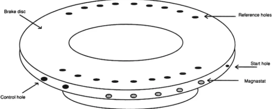
Two sets of holes were drilled radially towards the centre of a brake disc of a VOLVO 200 series passenger car, with a displacement of 180 degrees between them. Each set consisted of eight holes. The magnastats for each temperature were forced into five of these holes. (See Figure 5.1.)

20

-

-ra e ISC - . _{- A Reference holes}

Start hole - - ° (_ -- -. - - o - v Magnastat / . m Control hole .

Figure 5.1 Brake disc with magnastats and reference holes.

The first of the other three holes is used to generate a start pulse for the electric decoder and the last two generate check pulses for the decoder. There is sufficient space to drill additional holes if more magnastats are to be used, one between hole one and two and one between six and seven. The two check pulse holes can also be used for further magnastats.

5.2.2 Reference holes

Two groups, each of nine holes, were drilled axially approximately 4 cm from the outer edge of the brake disc (see Figure 5.1). Their purpose was to generate a reference signal for the decoder. The reference holes are somewhat displaced in relation to the magnastat holes, thus making it possible for the decoder to read the

magnastats at the correct time.

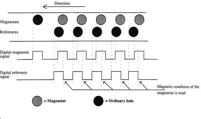
Figure 5.2 shows part of the brake disc, cut in such a way that the reference holes and the magnastats are placed in a row, and the position of the reference holes and magnastats in relation to each other. The figure also shows the two digital signals generated by the decoder.

21

/\

' |\ ' ' ' ' \ Magnetic condition of the

magnastat is read = Magnastat . = Ordinary hole

Figure 5.2 Position of reference holes in relation to magnastats. The corresponding digital signals generated and used by the decoder are shown at the bottom of the figure.

The purpose of the reference holes is to obtain a reading of the magnetic condition in the middle of the magnastat, independent of the angular velocity of the brake disc. Furthermore, it is easy to determine which magnastat is magnetic or non-magnetic.

An alternative procedure would have been to use only the row of magnastats. If the magnastats are placed according to increasing temperature, the number of pulses after the start pulse is counted and the temperature is then determined.

It is also possible to adjust the distance between the sensors laterally, thus displacing the magnastats half a magnastat in relation to each other. The method was not used in this study.

22

5.3 Sensor

An antilock brake system (ABS) wheel speed sensor from WABCO is used as a sensor in order to detect the magnetic state of the magnastats. The reason why an ABS sensor was chosen was among other things, that it is designed to cope with the environmental strain in a location close to vehicle brakes. It also withstands relatively high temperatures, approximately 180°C. The disadvantage of the ABS sensor in question is that it is quite large, approximately 1.5 cm x 4 cm.

OUTPUT

TÅHGET

POLE

CO"-Figure 5.3 Principal design of an ABS sensor [7:15].

The sensor consists basically of a permanent magnet and a coil (see Figure 5.3). When a magnastat drilled into the brake disc passes the sensor, the magnetic flux through the coil is changed depending on the magnetic state of the magnastat, which in turn causes a voltage u = -do/dt (Faraday's law).

23

Non-magnetic magnastats Magnetic magnastat

Side view of brake disc

Analogue signal from the ABS sensor

Figure 5.4 The analogue signal from the sensor consists of voltage pulses corresponding to the transitions from non-magnetic to magnetic material or vice versa.

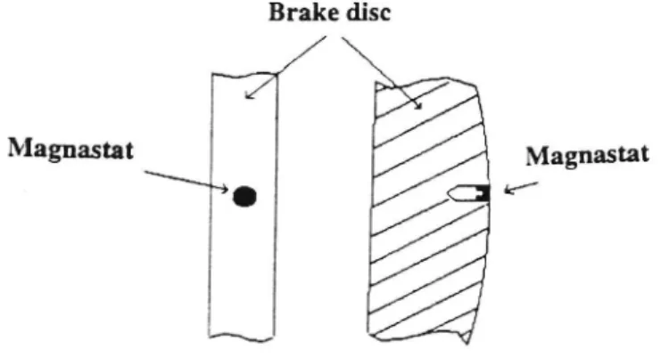
The shape of the sensor signal depends on the installation of the magnastat and the magnetic condition of the magnastat (Figure 5.4). If the magnastat is pressed into a hole in the disc, as in Figure 5.5, so that the upper surface of the magnastat is on a level with the disc surface, the sensor will sense a magnetic state caused by the iron of the brake disc, before the magnastat has arrived.

Brake disc

Magnastat

Figure 5.5 Part of the brake disc seen from two sides with the magnastat installed.

If the temperature is below the Curie temperature of the magnastat, the magnastat will also be considered as magnetic. Consequently, the magnetic flux from the ABS sensor will not be changed and no voltage is generated from the sensor.

24

If the temperature exceeds the Curie temperature of the magnastat, a sensor signal will be generated as a transition from magnetic to non-magnetic state is obtained.

The same condition is obtained when the rear edge of the magnastat passes the sensor, except for the difference that there is a transition from non-magnetic to magnetic material. Compared with the previous case, a signal with reversed polarity is obtained.

Similarly, the reference holes give rise to the same type of signal from the sensor as air is non-magnetic.

Another alternative is to place the magnastats as small elevations e.g. on a brake drum as in Figure 5.6. The sensor is now at a greater distance from the brake drum, and as a consequence the sensor senses a non-magnetic condition when no magnastat passes. The sensor signal will thus be obtained when the temperature is below the Curie temperature ofthe magnastat and the magnastat is magnetic. In the same way, small pieces of iron can be used instead of reference holes.

Brake drum <___

I = Iron

Magnastat

Figure 5.6 Part of a brake drum seen from the side with magnastats and reference pieces of iron.

25»

5.4 Sensor support

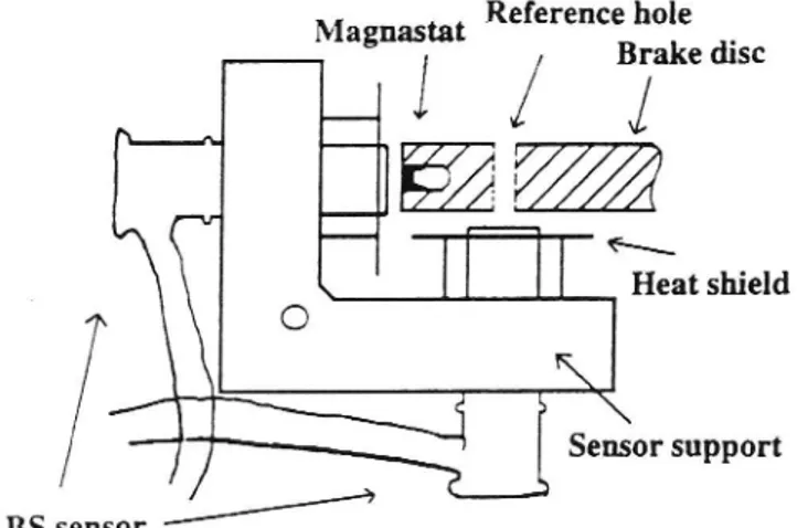
The sensor ñxture is made of steel and holds two ABS sensors, one for the row of magnastats and one for the row of reference holes (see Figure 5.7). The ñxture is connected to a support, which enables the positioning of the ñxture in almost any position. Two thin discs with holes for the sensors are installed at the front of the sensors. The purpose of the discs is to act as heat shields in order to avoid overheating of the sensor itself.

The sensor holder with the sensors is installed at the edge of the brake disc. One sensor point is located approximately 3 mm from the row of holes and the other sensor point at the same distance from the row of magnastats.

Magnastat Reference hole

I

' /

Blakedisc

521W

\

i)

\

Figure 5.7 Sensor ñxture with two ABS sensors installed.

26

5.5 Electric decoder

5.5.1 Introduction

In order to interpret the analogue signals from the ABS sensors, an electric decoder is used which converts the analogue signals to digital signals and then

processes them. The reference hole signal enables the decoder to decide the

magnetic state of each magnastat. The result is then presented via light emitting

diodes (LEDs). If the LED for 500°C is lit, the temperature of the brake exceeds 500°C.

The number of magnastats that can be detected by the decoder is limited to nine by the electronics.

The decoder also has an output for the digital signals and a trigger signal, thus making it possible to study the digital signal on an oscilloscope together with the corresponding analogue signal, which is of vital importance for the adjustment of suitable trigger levels.

5.5.2 Block diagram

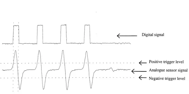
In Figure 5.9, the design of the decoder is represented as a block diagram. The input unit converts the analogue signals from the ABS sensor to digital pulses. Figure 5.8 shows the generation of the pulses through the high level of the digital signal when the analogue signal exceeds a positive trigger level. In the same way, the digital signal is set to zero when the analogue signal is below a negative trigger level.

27

<__ Digital signal

_ _ - . . . _ . . . - - <- Positive trigger level

F Analogue sensor signal

. . . - - - _{- - - <- Negative trigger level}

Figure 5.8 The digital signals are formed by the analogue signals being either above or below a positive or negative trigger level, respectively.

The trigger levels are adjustable as the amplitude of the sensor signal is very sensitive to the distance between sensor and brake disc. Furthermore, the angular velocity of the brake disc influences the amplitude, with the result that measurements cannot be carried out when the brake disc is at rest or moving slowly.

When the magnastat is non-magnetic, a digital pulse is generated with a pulse width approximately the same as the time required for the magnastat to pass the sensor. This is also valid for the reference holes as air is non-magnetic.

28

Analogue input signals

Mag Ref

Input unit

'

I

Control logic

.

'

l

I Reset Adjust upwards |

'

I

I

Decoder

l

l

l

I

A1-A9

l

R

l

I

Memory

ca

l

l

---

_lm-1;---Output unit

Figure 5.9 Block diagram for the electric decoder.

The control logic consists of a sequential net determining when it is time to read the condition of a magnastat. Furthermore, the control signals required for other blocks are generated.

29

The counter knows which of the nine magnastats to be detected.

The decoder addresses the memory cell indicated by the counter.

The memory stores the detected condition of the magnastat until it is time for a

new detection of the same magnastat. If the magnastat is non-magnetic, a zero is stored in the memory, otherwise the figure one.

The output unit presents the contents of the memory, i.e. the latest reading of the condition of the magnastats, on LEDs.

5.5.3 Circuit diagram

Appendix l shows the circuit diagram for input unit, output unit, voltage and clock generation. Since the Mag and Ref signals are treated in the same way, only

one of the connections is shown.

An operational ampliñer connected as a Schmitt trigger converts the analogue signal to a square signal. The output signal is +5 V when the analogue input signal exceeds the positive trigger level and -5 V when the analogue signal is below the negative trigger level. The absolute value of the positive and negative trigger level, respectively, is the same and is decided by the 100 K potentiometer. The trigger level can be varied between 0 and 5 volts.

The square signal is then converted to a digital signal between 0 and 5 volts with the TTL circuit 7414, which is also a Schmitt trigger. Finally, the digital signal is synchronised by the internal clock of the decoder, i.e. an ordinary D-type tlip-flop logic is clocked by a system clock. The synchronisation is necessary to reduce the risk of metastable conditions in the digital design.

30

The steering logistics, counter, decoder and memory blocks are all implemented in a PAL CE610H-15PC. Appendix 3 shows the ABEL program for the PAL circuit and Appendix 4 the Boolean equations. Appendix 5 shows the pin configuration of the PAL circuit.

Appendix 2 shows the condition graph for the sequential net of the steering logic.

When the start hole is detected, condition zero begins and the counter is set to zero. The subsequent sequence is then performed till the next start hole is met. For

each lap, the counter is incremented one step and the condition of the

corresponding magnastat is stored in the memory for the negative flank of the

reference signal.

The output unit (see Appendix l, page 2) consists of inverter, LED and resistance. When Ll is high, zero voltage is obtained on the output of the inverter and a current flows through the LED.

The negative supply voltage to the operations ampliñers is obtained by means of the ICL 7662 CPA, which is a voltage converter.

6

MEASUREMENTS

6.1 Introduction

The measurements were carried out by Lars-Gunnar Stadler and the author with assistance from personnel from VOLVO Car Corporation. The measurements were carried out in the test laboratory for disc brakes at VOLVO Car Corporation in Gothenburg.

3 1 6.2 Test design

The brake disc prepared with magnastats and holes was installed in one of the test rigs used for brake disc tests at VOLVO Car Corporation.

The two ABS sensors were mounted on the purpose-made ñxture, where one sensor recorded the row of reference holes and the other the row of magnastats. The signals from the ABS sensors were then connected to an oscilloscope, a PC for storing oscilloscope pictures of interest, and to the purpose-made signal processor.

The temperature of the brake disc was measured with a thermoelement of the sliding sensor type installed on the side of the brake disc to be used as reference temperature. The reference temperature was presented on a digital display.

6.3 Performance

The brake disc was heated to fully 600°C by braking at a speed equivalent to 40 km/h. Braking then ceased and the temperature started falling. The angular velocity of the disc during the cooling period corresponded to a driving speed of 20 km/h.

6.4 Documentation

In order to document the test, a video camera was used and the oscilloscope showing the analogue output signal of the ABS sensor and the digital output signal of the signal processor were recorded on video together with the reference temperature and the LEDs on the signal processor. Interesting oscilloscope pictures were stored on a PC.

32

6.5 Results

The test results were evaluated by studying the video recording of the test, compiled in Table 1. Temperatures were read during the cooling period.

The column Rated temperature of magnastat in °C states the Curie temperature

of the magnastat. Sliding temperature sensor in °C consists of the columns

Full , 3/4 , 1/2 and No signal . Full means temperatures read from the reference sensor when the signal from the ABS sensor just begins to be lowered. 3/4 means the temperature when the ABS sensor was lowered to 3/4 of full signal strength, etc. The temperature difference between Full and No signal is the recorded change interval for the respective magnastat.

Rated temperature Deviation Sliding temperature sensor in °C

of magnastat in °C rated temp. Full 3/4 1/2 1/4 No signal

227 -35 270 265 262 261 260

327 +6 331 326 321 319 317

427 +42 397 388 385 383 381

527 +91 442 439 436 433 431

627 +147 487 483 480 477 473

Table 1 Compilation of transition temperatures.

From the table, it can be seen that the transition interval for all magnastats is approximately 15°. It should be noted though, that the sensor signal is reduced from 3% to 1%: of strength in only 6°, which indicates a relatively fast transition.

The rated temperature of the magnastat does not, however, agree very well with the reference temperature. The column Deviation rated temp , which contains the difference between rated temperature and the 1/2 column, shows that especially the 6270 magnastat has a deviation of approximately 150°. This is probably due to the fact that the sliding sensor is in close contact with the surface

33

especially the 627° magnastat has a deviation of approximately 150°. This is probably due to the fact that the sliding sensor is in close contact with the surface of the disc, while the magnastat is drilled into the disc. Furthermore, the

magnastats are fixed approximately 4 cm from each other radially, which gives rise to both time delay and cooling. This influences the result even more with increasing temperature. It should be noted though, that the transition temperatures were the same in repeated tests.

7

SUMMARY AND DISCUSSION

The above measurements show that the described method of monitoring

temperature with the aid of the Curie-Weiss effect works well as the transition

interval of the magnastats turned out to be 15°C or less, which is quite insigniñcant considering the large temperature variations -in a vehicle brake. The method is most suitable when only a limited number of temperatures are of interest, which is the case for a brake temperature system where a few different temperatures are sufficient to define criteria for warning of conditions such as fading, worn brake linings and uneven brake force of the different brakes [8].

The method is simple, robust and not dependent on calibration, which guarantees high reliability. What is needed is a magnastat with desired Curie temperatures and a sensor to detect the magnetic state of the magnastats.

The calculation of the temperature time history in the brake disc is quite simple as time can easily be measured by means of the system electronics or with a computer used for evaluating sensor signals.

The method is, however, not suitable for measurement when a continuous temperature scale is desired. In order to achieve sufficient precision, a considerable number of magnastats would be required, which would be unmanageable.

34

In a possible second phase of the project, where the aim is to produce an adequate brake monitoring temperature system, it is suggested that new tests should be carried out in a test rig for brakes, but with the reference sensor installed in the same way as the magnastats in order to be able to determine the transition interval of the magnastats with greater precision. Furthermore, accurate criteria for the detection of functional errors in the braking system should be developed with the aid of temperature levels, temperature gradients and temperature differences between brakes in the brake system. Finally, accurate field studies must be carried out in order to determine the reliability of the monitoring system.

The ferromagnetic alloys Cu-Ni and Co-Ni have Curie temperatures between O°C and 950°C with no structural change, which makes it possible to tailormake materials with desired Curie temperatures for brake applications. If more suitable material cannot be found in a continued material study, some copper-nickel and cobalt-nickel alloys should be made and evaluated.

35

REFERENCES

1 S. Chikazumi, 'Physics of Magnetism', John Wiley & Sons (1964).

2 R.M. Bozorth, 'Ferromagnetism', D. Van Nostrand

Company (1951).

3 D.K. Cheng, 'Field and Wave Electromagnetics', 2nd ed, Addison-Wesley Publishing Company (1989).

4 1993 SAE HANDBOOK, Volume 2, SAE J661 AUGS7, SAE. SAE J843 NOV90.

5 'Binary Alloy Phase Diagrams', 2nd ed, ASM International.

6 CJ. Smithells, 'METALS REFERENCE BOOK

VOLUME II', 4th ed, Butterworth & Co (1967).

7 J. Ormerod, R. Taylor, J. Roozee, 'Improvments and

Applications of Permanent Magnet Materials in Automotive Sensors',

SAE Technical Paper Series 920171.

8 K-H. Wollenweber, R. Leiter, 'Function-monitoring brake

system: temperature monitoring brake system', I Mech E 1993-2.

Appendix 1

Page 1(3)

Circuit diagram for the electronic decoder Circuit diagram for the input unit and clock generator

Mag ' ' ,

O--Ä'

1

IOK

II

?2 4!

!5

DigitalMag

3 LM324

_Ej-le

0-7-9 D

.

0

'

I

I

T

i

i

Clk

v

-

l

,

,

I

100 K | 7414 | 1 74374 '

| Hex Schmitt . . Octal D-type '

. triggerinverteq I Hip-flop

|

.

.

Ref

6

.

1

|

lClk I

O--> '

7

IOK 9

8 3

v

'2

DigitalRef

5 LW

_EJ-'rä 1=] 0-.--.e D

*

o

+

'

|

'

I

I

-

I

I '

F

o

6

o

Appendix 1

Page 2(3)

Circuit diagram for the output unit

O +5v ' ' K K

L1

I

|

820

M

:

I D

I

N

L2

i

|

820

Kl;

:

| I: i I

I:

N

L3

i

1

820

RMK

0

i D0 I

E

N

i 7414

i

'

|

, Hex

I

Appendix 1 Page 3(3)

Circuit diagram for voltage generation

0

7805

0

O

O

O

8

_ålzlo uF

0

nr)

Appendix 2

Page 1(1)

Flowchart for the sequential net of the decoder Flowchart for the sequential net controlling the electronic decoder

Input signals: (Ref, Mag)

Ref is the digital and synchronous signal from the reference line sensor.

Mag is the digital and synchronous signal from the magnastat line sensor. SO: START

(1,-)

(_ 1)

s1: Wait till

Appendix 3 Page 1(2)

ABEL program for the sequential net of the decoder module tempmet

title 'tempmet'

tempmet device 'E0600';

clkl,clk2 pin 1,13; "Insignal klocka

ll,12,13,l4,15,16,l7,18,l9 pin 15,16,17,18,19,20,21,22,10; " Lagrar lysdiodens värde

mag,ref pin 2,11; "Insignal magnastat

och referensrad

q1,q2,q3

pin 9,8,7; "Tillstånds vipporna

rl,r2,r3,r4 pin 6,5,4,3; "4-bitsräknare

l1,12,13,l4,15,16,l7,18,l9 istype 'reg';

q1,q2,q3 istype'reg'; rl,r2,r3,r4 istype 'reg';

q=[q1,q2,q3]; "Deñnierar q som en vektor

r=[r1,r2,r3,r4]; "Deñnierar r som en vektor

1=[ll,12,13,l4,15,16,l7,18]; "Deñnierarl som en vektor

sO=O;sl=1;32:2;s3=3;s4=4;35=5;sö=6;s7=7; equaüons

l.CLK=clk2; "Kopplar ih0p D-vippernas

l9.CLK=clk1; "klecksignal med kretsens

r.CLK=clkl; "klocksignal

q.CLK=clk1 ;

when ((q.FB==4) & (r.FB==1)) then 11:=!mag; else ll:=ll.FB; when ((q.FB==4) & (r.FB==2)) then 12:=!mag; else 122=12.FB; when ((q.FB==4) & (r.FB==3)) then l3:=!mag; else l3:=l3.FB; when ((q.FB==4) & (r.FB==4)) then l4:=!mag; else l4:=l4.FB; when ((q.FB==4) & (r.FB==5)) then 15:=!mag; else 15:=15.FB; when ((q.FB==4) & (r.FB==6)) then 16:=lmag; else 16:=l6.FB; when ((q.FB==4) & (r.FB==7)) then l7:=!mag; else l7:=l7.FB; when ((q.FB==4) & (r.FB==8)) then l8:=!mag; else l8:=18.FB; when ((q.FB==4) & (r.FB==9)) then l9:=!mag; else 19:=l9.FB;

state_diagram q state sO: r:=O;

case !ref & !mag ref# mag :sO; endcase;

state sl: r:=r.FB;

case ref & !mag :52; !ref& !mag :sl; magnastaten" mag :sO; endcase; state s2: r:=r.FB; case ref :sZ; !ref :s3; endcase; state s3: r:=(r.FB+1); goto s4; state S4: r:=r.FB; goto 55; state s5: r:=r.FB; case !mag :s 1; mag 235; endcase; state s6: goto SO; state s7: goto sO; end

VTI Notat 35A- 1994

Appendix 3

Page 2(2)

"Nollställer

räknaren och väntar"

:sl; "tills både ref och

mag är låga"

"Väntar på att ref ska bli

"hög eller att start "ska dyka upp"

"Vänta på att ref ska bli

låg"

"Räkna upp räknaren 1 steg

"Läs av magnastaten"

"Väntar på att ev hög

"magnastat ska bli låg"

"Ej använt tillstånd "Ej använt tillstånd

ABEL 4.20 - Device Utilization Chart

tempmet

Appendix 4

Page 1(4)

The Boolean equations for the sequential net of the decoder Thu Nov 25 17:19:22 1993

==== E0600 Prcgrammed Logic ====

ll.D =( !mag & q1.FB & !q2.FB & !q3.FB & !r1.FB & !r2.FB & !r3.FB & r4.FB

ll.C 12.D l2.C 13.D l3.C Il # i t ät åt ät i t i t # i tåt i t i t i ti t l l

!r4.FB &11.FB

r3.FB &11.FB

r2.FB &11.FB

r1.FB &11.FB

q3.FB &11.FB

q2.FB &11.FB

!q1.FB &11.FB ); " ISTYPE 'BUFFER'

( Clk2 );

( !mag & q1.FB & !q2.FB & !q3.FB & !r1.FB & !r2.FB & r3.FB & !r4.FB

r4.FB &12.FB

!r3.FB &12.FB

r2.FB & 12.FB

r1.FB &12.FB

q3.FB &12.FB

q2.FB &12.FB

!q1.FB &12.FB ); " ISTYPE 'BUFFER'

=( clk2 ); ll # i t i ti t i t i t i t l

l ( !mag & q1.FB & !q2.FB & !q3.FB & !r1.FB & !r2.FB & r3.FB & r4.FB

!r4.FB &13.FB

!r3.FB & 13.FB

r2.FB & 13.FB

r1.FB & l3.FB

q3.FB & l3.FB

q2.FB &13.FB

!q1.FB & l3.FB ); " ISTYPE 'BUFFER'

( clk2 );

l4.D l4.C 15.D 15.C 16.D 16.C l7.D l7.C 18.D 18.C 19.D Appendix 4

Page 2(4)

( !mag & q1.FB & !q2.FB & !q3.FB & !r1.FB & r2.FB & !r3.FB & !r4.FB r4.FB & l4.FB r3.FB & l4.FB !r2.FB & l4.FB rl.FB & l4.FB q3.FB & l4.FB q2.FB & l4.FB

!q1.FB & l4.FB ); " ISTYPE 'BUFFER' ( clk2 ); Il : t i t i t åt ät ät ät l l

( !mag & q1.FB & !q2.FB & !q3.FB & !r1.FB & r2.FB & !r3.FB & r4.FB

!r4.FB &15.FB

!r2.FB &15.FB

rl.FB &15.FB

q3.FB &15.FB

q2.FB &15.FB

!q1.FB &15.FB ); " ISTYPE 'BUFFER'

( clk2 );

( !mag & q1.FB & !q2.FB & !q3.FB & !r1.FB & r2.FB & r3.FB & !r4.FB

r4.FB & 16.FB ' !r3.FB & 16.FB !r2.FB & 16.FB rl.FB &16.FB q3.FB & 16.FB q2.FB & 16.FB

!q1.FB & 16.FB ); " ISTYPE 'BUFFER' = ( clk2 ); #át ät it itit ät ll

( !mag & q1.FB & !q2.FB & !q3.FB & !r1.FB & r2.FB & r3.FB & r4.FB !r4.FB & l7.FB !r3.FB & l7.FB !r2.FB & l7.FB rl.FB & l7.FB q3.FB & l7.FB q2.FB & l7.FB

!q1.FB & l7.FB ); " ISTYPE 'BUFFER' ( clk2 ); II * t ät i t i t i ti t ät l l

-( !mag & q1.FB & !q2.FB & !q3.FB & rl.FB & !r2.FB & !r3.FB & !r4.FB r4.FB &18.FB r3.FB &18.FB r2.FB &18.FB !rl.FB &18.FB q3.FB &18.FB q2.FB & 18.FB

!q1.FB & 18.FB ); " ISTYPE 'BUFFER'

=( clk2 );

=( !mag & q1.FB & !q2.FB & !q3.FB & rl.FB & !r2.FB & !r3.FB & r4.FB VTI Notat 35A- 1994

l9.C r1.D r1.C r2.D r2.C # äi t it i h ät i t Appendix 4 Page 3(4)

!r4.FB & l9.FB

r3.FB &19.FB

r2.FB &19.FB

!r1.FB & 19.FB

q3.FB & 19.FB

q2.FB & l9.FB

!q1.FB & l9.FB ); " ISTYPE 'BUFFER'

=( Clkl );

:( !q1.FB & q3.FB & rl.FB & !r2.FB

# i t ät i t i t i

t !q1.FB & q3.FB & rl.FB & !r3.FB

!q1.FB & q3.FB & rl.FB & !r4.FB

!q1.FB & q2.FB & q3.FB & !r1.FB & r2.FB & r3.FB & r4.FB q1.FB & !q2.FB & rl.FB

!q1.FB & q2.FB & !q3.FB & rl.FB

!q2.FB & q3.FB & rl.FB ); " ISTYPE 'BUFFER' =( clkl );

:t

ti

ti

tät

it

n

!q1.FB & q2.FB & q3.FB & !r2.FB & r3.FB & r4.FB !q1.FB & q2.FB & !q3.FB & r2.FB ' q1.FB & !q2.FB & r2.FB

!q2.FB & q3.FB & r2.FB ); " ISTYPE 'BUFFER' =( clkl );

Appendix 4 Page 4(4) r3.D =( !q1.FB & q3.FB & r3.FB & !r4.FB

# !q1.FB & q2.FB & q3.FB & !r3.FB & r4.FB # !q1.FB & q2.FB & !q3.FB & r3.FB

# q1.FB & !q2.FB & r3.FB

# !q2.FB & q3.FB & r3.FB ); " ISTYPE 'BUFFER' r3.C =( clkl );

r4.D =( !q1.FB & q2.FB & q3.FB & !r4.FB

# !q1.FB & q2.FB & !q3.FB & r4.FB

# q1.FB & !q2.FB & r4.FB

# !q2.FB & q3.FB & r4.FB ); " ISTYPE 'BUFFER'

r4.C =( Clkl );

q1.D =( !q1.FB & q2.FB & q3.FB # q1.FB & !q2.FB & !q3.FB

# mag & q1.FB & !q2.FB ); " ISTYPE 'BUFFER' q1.C =( clk1);

q2.D =( !mag & ref & !q1.FB & !q2.FB & q3.FB

# !q1.FB & q2.FB & !q3.FB ); " ISTYPE 'BUFFER' q2.C =( clkl );

q3.D =( !ref& !q1.FB & q2.FB & !q3.FB # !mag & !ref& !q2.FB

# q1.FB & !q2.FB ); " ISTYPE 'BUFFER' q3.C =( clk1);