Vision based facial emotion detection using deep convolutional neural networks

(1)

M

ÄLARDALEN

U

NIVERSITY

S

CHOOL OF

I

NNOVATION

,

D

ESIGN AND

E

NGINEERING

V

ÄSTERÅS

,

S

WEDEN

Examensarbete för kandidatexamen i datavetenskap – 15 HP

Vision based facial emotion detection using deep

convolutional neural networks

Fredrik Julin

Fjn14001@student.mdh.se

Examiner: Mobyen Uddin Ahmed

Mälardalen University, Västerås, Sweden

Supervisor: Hamidur Rahman

Mälardalen University, Västerås, Sweden

(2)

2

Fredrik Julin Vision based facial expression detection using

deep convolutional neural networks

Abstract

Emotion detection, also known as Facial expression recognition, is the art of mapping an emotion to some sort of input data taken from a human. This is a powerful tool to extract valuable information from individuals which can be used as data for many different purposes, ranging from medical conditions such as depression to customer feedback. To be able to solve the problem of facial expression recognition, smaller subtasks are required and all of them together form the complete system to the problem. Breaking down the bigger task at hand, one can think of these smaller subtasks in the form of a pipeline that implements the necessary steps for classification of some input to then give an output in the form of emotion. In recent time with the rise of the art of computer vision, images are often used as input for these systems and have shown great promise to assist in the task of facial expression recognition as the human face conveys the subjects emotional state and contain more information than other inputs, such as text or audio. Many of the current state-of-the-art systems utilize computer vision in combination with another rising field, namely AI, or more specifically deep learning. These proposed methods for deep learning are in many cases using a special form of neural network called convolutional neural network that specializes in extracting information from images. Then performing classification using the SoftMax function, acting as the last part before the output in the facial expression pipeline. This thesis work has explored these methods of utilizing convolutional neural networks to extract information from images and builds upon it by exploring a set of machine learning algorithms that replace the more commonly used SoftMax function as a classifier, in attempts to further increase not only the accuracy but also optimize the use of computational resources. The work also explores different techniques for the face detection subtask in the pipeline by

comparing two approaches. One of these approaches is more frequently used in the state-of-the-art and is said to be more viable for possible real-time applications, namely the Viola-Jones algorithm. The other is a deep learning approach using a state-of-the-art convolutional neural network to perform the detection, in many cases speculated to be too computationally intense to run in real-time. By applying a state-of-the-art inspired new developed convolutional neural network together with the SoftMax classifier, the final performance did not reach state-of-the-art accuracy. However, the machine-learning classifiers used shows promise and bypass the SoftMax function in performance in several cases when given a massively smaller number of samples as training. Furthermore, the results given from implementing and testing a pure deep learning approach, using deep learning algorithms for both the detection and classification stages of the pipeline, shows that deep learning might outperform the classic Viola-Jones algorithm in terms of both detection rate and frames per second.

(3)

3

List of figures

Figure 2.1 – Artificial intelligence subareas ... 9

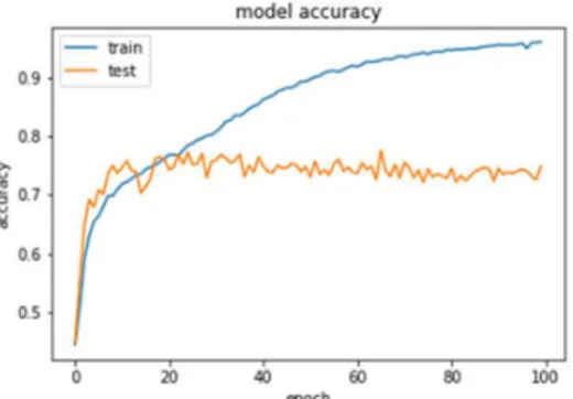
Figure 2.2 - Overfitting seen in a graph given from a training session of a CNN ... 11

Figure 2.3 - A simple overview of an ANN architecture ... 13

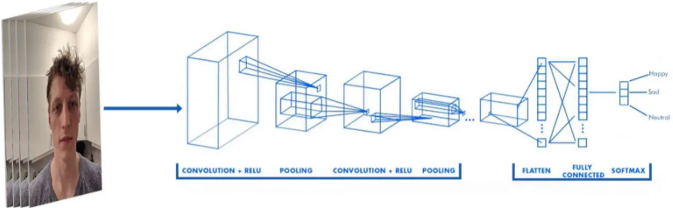
Figure 2.4 - An example pipeline of a CNN using images of faces as input ... 14

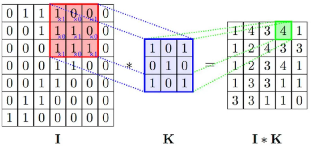
Figure 2.5 - A single kernel(K) applied to the input(I) ... 15

Figure 2.6 - Rectified linear function (ReLU) ... 16

Figure 2.7 - Max pooling applied to a 4x4 matrix ... 17

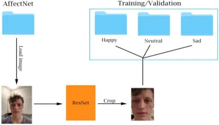
Figure 5.1 - Non-FER images from AffectNet dataset ... 23

Figure 5.2 - Misclassifications from the manually annotated set. From the left, Happy, Sad, Neutral ... 23

Figure 5.3 - Illustration of the detection and ROI extraction preparing the dataset for classification ... 24

Figure 5.4 - 4 Valid augmentation techniques from the left and the last one being a bad example ... 25

Figure 5.5 - VGG16 architecture with all layers frozen but the last conv layer and swapped the last FC... 25

Figure 5.6 - Final CNN model architecture ... 26

Figure 6.1 - Failed detections on AffectNet dataset ... 30

Figure 6.2 - Overfitting occurrence of VGG16 trained on AffectNet ... 30

Figure 6.3 - Model loss and accuracy from training/validation ... 31

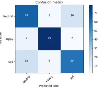
Figure 6.4 - CNN CM ... 31

Figure 6.5 - Logistic regression solver sag CM ... 32

Figure 6.6 - SVM poly kernel CM ... 33

Figure 6.7 - Random Forest using 100 N estimators CM ... 33

Figure 6.8 - Decision tree CM ... 34

Figure 6.9 - KNN(K=24) CM... 35

Figure 6.10 - Naive multinomial CM ... 35

Figure 6.11 - Real-time classification using DL for detection and classification ... 36

Figure 6.12 - Real-time detection results angles ... 36

Figure 6.13 - Real-time detection illumination test, from the top 46 lux down to 1 ... 37

Figure 9.1 - Down sampling using max pooling operation in a CNN layer ... 45

Figure 9.2 - Relation between SoftMax regression and logistic regression ... 45

Figure 9.3 - Linear regression between dependent variable weight(y) and independent variable height(x) ... 46

Figure 9.4 - Logistic regression with sigmoid function applied between passing an exam and hours studied ... 46

Figure 9.5 - KNN using K=3 to determine X ... 46

Figure 9.6 - Real-time detections ResNet vs Viola-Jones ... 47

Figure 9.7 - FER2013 public test set result CM ... 47

Figure 9.8 - FER2013 private test set result CM ... 48

List of tables

Table 5.1 - Number of samples in the AffectNet manually annotated dataset for 3 emotion classes ... 22

Table 5.2 - Number of samples in the FER2013 test sets for 3 emotion classes ... 23

Table 6.1 - Detection algorithms benchmark ... 29

Table 6.2 - Test accuracy of CNN on test sets... 30

Table 6.3 - Logistic regression solvers ... 32

Table 6.4 - SVM kernels ... 32

Table 6.5 - Random forest ... 33

Table 6.6 - Decision tree classifier ... 34

Table 6.7 - KNN ... 34

Table 6.8 - Naive Bayes ... 35

Table 6.9 - Real-time classification ... 36

(6)

6

List of abbregations

AI

Artificial intelligence

FER

Facial expression recognition

ROI

Region of interest

ANN

Artificial neural network

CNN

Convolutional neural network

RNN

Recurrent neural network

DL

Deep learning

ML

Machine-learning

SVM

Support vector machine

KNN

K-nearest neighbor

(7)

7

1. Introduction

The number of areas utilizing computer vision for image related problems has expanded rapidly in the last decade, now integrated into systems ranging from self-driving cars to the detection of tumors in radiographs. Being able to automate tasks that the human visual system can perform and perhaps even beyond that of the human capabilities is a powerful tool indeed, as it opens possibilities that previously were only speculated in. One could say computer vision is the art of not only making a computer “see” but also imparting human intelligence of processing input. With the rise of AI, the subareas of Machine Learning and Deep Learning, the potential to integrate intelligent models with computer vision systems has become a popular method to handle increasingly complex application areas. One area that has been getting a rising amount of attention for its many potential applications is the art of detecting the emotional state of humans depending on their faces. This task is known as emotion detection or Facial expression recognition (FER) and is what this thesis work will revolve around.

To be able to detect and recognize expressions in a human face is a powerful tool that has potential use in a wide range of applications and industries. FER is the practice of using computers to map certain expressions using images or video footage of the human face. This technology is showing large potential when applied to tasks such as human-abnormal behavior detection, computer interfaces, autonomous driving, intelligent tutoring systems, health management, and other similar assignments [1, 2].

A typical FER system consists of face image acquisition, pre-processing, feature extraction, training, and classification [1, 3, 4]. To be able to get an accurate mapping of an expression to the face, the input data and feature extraction from the region of interest (ROI) must be performed before any form of classification can begin as the recognition task builds upon on how well the first two steps are performed [4]. It is especially important for real-time application of FER as it involves detecting the face and performing feature extraction from a constant stream of frames while uncontrolled conditions may apply, for example, but not limited to, uncontrolled movement, different poses, and change in lightning. When these uncontrolled conditions occur, it may prove more challenging to perform the detection of the face(s) in the frames collected from the video footage. This, in turn, will affect how well one can extract the desired ROI if it is possible at all. These challenges are added to what is already considered to be difficult in the FER problem, such as the variety of sizes, and shapes for the human face. Facial detection is the first step of any FER and can be described as two smaller subtasks [5]. The first being the actual detection of the face and the second being to extract the region of interest (ROI) from the detected face by creating a bounding shape around the components that are part of the ROI, in this case, the nose, eyes, eyebrows, and mouth (also known as facial landmarks).

When the features have been extracted, one can start to look at the expression of the face in the images. There is a range of different algorithms and techniques to handle classifying the expression in the images, depending on the features extracted and used for the classification. A promising and well-studied strategy that has been applied and proven to be very accurate is to train a system to recognize expressions by using deep learning [6]. In deep learning, an Artificial Neural Network (ANN) can be applied through mimicking the work-flow of neurons in the human brain and map inputs to outputs by processing the input through a set of interconnected hidden layers containing neurons (or nodes) that activate depending on the data input. In this report, the neurons will be referred to as nodes. When using images as input data, a type of specialized ANN called Convolutional Neural Network (CNN) has been increasingly popular to apply for feature extraction and classification [7-9]. CNN's accept tensors as input into the network and just as with ANNs in general, the CNN contains several hidden layers that perform a range of distinctive calculations and feature extractions on the data.

After the features of the face(s) are extracted from the input image to a CNN, a SoftMax function is frequently used as a classifier. In exploring the possibilities for higher accuracy for the classification process, a set of machine learning classifiers replacing the SoftMax layer are purposed. Therefore, using CNN's as feature extractor, this set of classifiers have been trained and evaluated on a dataset. In this process, different ways to improve the CNN feature extraction for giving optimal features to the machine learning algorithms have been analyzed. Using FER in real-time systems could potentially open doors for many new application areas, e.g. within mental health-related areas. To explore how practical deep learning models can be deployed for such potential systems an algorithm using deep learning for face detection and classification in a real-time system have been implemented and evaluated.

(8)

8

2. Background

In this section, the intuition behind neural networks, machine-learning and important concepts of computer vision and image processing will be described in detail.

2.1. Datasets

When choosing a data collection to work with for classification purposes, there are two major categories that can be considered. One being datasets created in a lab or controlled environment (e.g. CK+) and the other being a set of images that are taken in the “wild”, meaning they are taken from an uncontrolled environment (e.g. FER2013 and AffectNet)[10-12].

2.2. Image preprocessing

To be able to accurately map an emotion to facial expressions in an image, the first step is to find a way to process the data from the image to prepare the data for proper classification in the next stages of the process. Before deep learning(DL) was starting gaining increased popularity in FER, you would extract your own features manually based on an image pre-processing step before feeding these features into your classifier[13, 14]. In this work, the feature extraction is done by the CNN automatically and the only pre-processing steps taken before extraction are face detection and alignment, image resizing and finally cropping.

2.2.1. Face detection

Face detection can be regarded as a special case of object-class detection. In object-class detection, the task is to find the locations and sizes of all objects in an image that belongs to a given class (e.g. car, face, animal etc.).

Before being able to inspect faces for expressions and emotion, one must identify where the face resides in an image. Being able to distinguish a face from the rest of the human body, detect a face in an image or in everyday life (real-time) is a trivial task for the visual perception1_{of the human vision. However, the same task is a}

challenging one for a computer. This is challenging mainly due to two reasons: Firstly, the anatomy of the human face can differ greatly across different subjects, for example, things like size, shape, textures and, color. Secondly, in images, variation to lightning, pose and other varying properties can make the detection harder due to vast changes in the pixel values being looked at. These two challenges in combination make it hard to make face detection efficient, especially in real-time where exposure to several different circumstances may occur continuously (head movements, changes in light depending on pose etc). The detection step is not only a crucial part of FER but is also imperative for solving many other computer vision related problems, such as recognition and surveillance.

2.2.1.1. Viola-Jones Algorithm

There are many different approaches to detecting faces, a great breakthrough was accomplished with the viola-jones algorithm making use of “weak-classifiers” [15]. By using simple haar features, it can, after a great deal of training yield very promising results[16]. Plenty of training samples, both positive (images containing faces) and negative (images not containing faces) are required to make the best use of the algorithm. Viola-Jones is still considered to be very robust and accurate and has been used in many studies concerning different types on face detections and classification problems regarding the human face in the past [3, 7, 17].

2.2.1.2. Deep-learning based detection

Viola-Jones was first introduced back in 2001 and was considered a big breakthrough in object detection[15]. In more recent years, detection through DL has demonstrated more promising results as it is not as sensitive to the different conditions that may occur in an image mention earlier if trained properly. This new method enables more robust face detection in varying poses and varying lightning. This improved accuracy under varying conditions comes at the cost of more computational power required for the detection[18]. Both viola-jones and CNN’s are dependent on data to be trained upon to increase accuracy and robustness. However, there is a major difference in how the training occurs. The viola-jones uses AdaBoost which does not measure accuracy but rather only tries to minimize the loss, furthermore, the Haar-like features are predetermined features that no matter with how much training is given, will have trouble detection anything that deviates from full frontal faces with a set range of lightning. Since the CNN is not dependent on a set of predetermined features, it will have the ability to learn the characteristics of a face in positions deviating from full frontal, given that the training data is diverse enough to provide the CNN with these features. Although the CNN has much stronger capabilities when it comes to accurate

1_{Visual perception is the ability to interpret the surrounding environment using light in the visible spectrum reflected by the objects in the environment. (“Visual}

(9)

9

deep convolutional neural networks and robust detection, it comes at the cost of resources, especially in terms of memory. Depending on the device to run the face detection algorithm, this factor may impact the choice between choosing a CNN based approach or viola-jones.

2.2.2. Feature extraction

To be able to classify an emotion to a face in a given image, the first step is to pre-process the image to facilitate the course of extracting the desired features. Depending on what technique is being used to extract features, this process may involve converting images to grayscale format and applying additional filters and/or manipulations if needed (blurring, sharpening, resizing). These steps vary depending on the algorithm used to make the classification as different algorithms might benefit from different kinds of features extracted from the data when making the classification[14, 19, 20]. In the case of using CNN’s for classification, the CNN extract the features it deems important to the class by itself iteratively when passing training data through the network, without any manual pre-processing. Although, it is still possible to extract features first and then let the CNN learn from these manually extracted features to make features of its own[8].

When any potential pre-processing is finished, the second step is to simply input the image into the CNN and as mentioned the features will be extracted automatically. Depending on how many layers chosen for the architecture, alongside what the chosen properties for each layer are, the number of features and how they are interpreted will differ, this process will be covered in greater detail in section 2.3. When the detection and the feature extraction steps are finished, one can start to perform the desired operations on the extracted features. In this thesis work, that means using the features to classify what kind of emotion the expression on the detected face is reflecting (Happy, Sad or Neutral).

2.3. Machine learning

Machine learning (ML) can be described as a subarea of AI. Furthermore, deep learning (DL) can be regarded as a subarea within ML2_{. This order of areas can be observed in figure 2.1. Before explaining these notions, it is}

important to set out the differences between AI, ML, and DL. AI covers a very broad scope of concepts that specifically refers to the art of using computers to mimic the cognitive functions of the human brain(intelligence). In other words, AI can be described as a system and/or machine that carries out a set of tasks based on one or more algorithms that mimic intelligent behavior. ML, on the other hand, is part of the broad concept of AI but refers more specifically to the ability of these systems to learn for themselves, given an arbitrary set of data. This means that instead of having a set of predefined algorithms that run the same way every iteration, the algorithms are subject to change as they learn more about the data they are given to process. An important takeaway is that using an algorithm to predict an outcome based on some data is not ML. However, using the predicted outcome from the data provided to improve future predictions is ML.

Within ML, there are typically three different ways you can let your algorithms learn about the data you provide. These are supervised, unsupervised and reinforcement learning. This work is limited to working with supervised learning and will not delve into the other methods. Therefore, the reader of this report can assume that all the algorithms regarding ML and DP that are covered in the background section are all based on supervised learning. Supervised machine learning stands for many of the popular algorithms and techniques and algorithms that are used today and can be thought of as guiding the process with input training data(x) that maps to an output value(y). For supervised learning to work as intended, the correct output y corresponding to the input x is essential as it guides the learning process. Two of the most typical uses for supervised machine learning is classification and regression tasks[21].

Figure 2.1 – Artificial intelligence subareas

(10)

10

deep convolutional neural networks 2.3.1. Classification vs regression

ML can be used for classification and regression tasks, but it is important to know the difference between the two when deciding on a what model to use. A classification model has the task of mapping some input data to a discrete category or label. A typical example of a classification task would be what is being accomplished in this thesis work, that is, given an image of a face as input, mapping a label to the corresponding emotion to the face. In classification models it is common for the prediction output to be made as a probability of the labels involved, the result can then either be displayed as the probability for all the labels or simply take the highest probability and convert it into a class label as a single output. A regression model outputs a continuous real-valued, e.g. a floating-point value that can then be compared to other values. Most often these values are quantities, e.g. amounts, lengths or sizes[22].

2.3.2. Train, validation, and test

When a ML or DL model has been designed and the dataset with the corresponding input and output has been collected, it must be trained before it can be used to make any useful predictions. The data that has been collected for the model should be split into three smaller sets, each with a different purpose. In general, a good starting point is to split the set into an 80-203_{or 70-30 ratio, where the higher percentage of the set will be used for training and}

the lower is used for validation will be used for validation and testing[23]. The training set is very straightforward and is used just as it implies, to train the model to learn about the features that belong to the classes that are provided in the set iteratively.

During the training session, the model will also perform classification on the validation set. This classification will be performed using the information the model has learned about the data it has been trained on so far in the training set. The reason why the validation set is separate from the training set is so that we can validate the model’s current accuracy on data that the model is not familiar with from the training set that is used to update the learnable parameters. The most important purpose of the validation set is to keep the model from overfitting (this concept is covered in a few sections) to the data in the training set.

Finally, the test set is used to test the model’s final performance and robustness when the training and validation have been completed. When using the test set, the model is not given the corresponding output y to each input x, but instead must make the predictions based on what it has learned. This step is an absolute necessity for any model that is to be deployed and used in the field, as the entire purpose of a classification model is to be able to classify and label data without having information about the data beforehand.

2.3.3. Parameters and hyperparameters

In ML and DL, the two concepts of parameters and hyperparameters are important to grasp, as they have a significant impact on how well the model will perform. Parameters refer to a configurable variable that is internal to the model which value is determined based on the input data. This form of data is used when the model makes predictions, in DL, an example of parameters are the weights that are iteratively being updated throughout the training process.

Hyperparameters, on the other hand, are responsible for controlling how the parameters should be updated and assigned. One might think of the hyperparameters as being assigned and set before a model starts training or validating a dataset, and these, in turn, affect how the model learns and updates the internal parameters. Some examples on hyperparameters are the learning rate(α), number of iterations in training, hidden layers (𝑙), hidden units 𝑛[1], 𝑛[2] …. 𝑛[i], and choice of the activation function. These hyperparameters can be hard to estimate depending on the problem at hand and the way to an accurate model is often starting out with some initial values and performing trial and error tweaking of these hyperparameters to see how it affects the model accuracy. All hyperparameters have an impact on model accuracy. The learning rate will be discussed next, which affects how fast or slow the model updates the weights and learns.

2.3.3.1. Learning rate

The learning rate can be described as the path to minimizing the loss between the actual output and the predicted output from the training data. A typical start value to initiate models with usually ranges somewhere in between 0.01 – 0.0001. The learning rate is one of the hyperparameters and has a significant effect on how the weights of the model are updated. The main purpose of this hyperparameter in layman’s terms is to decide how small of a step the model should be updated with towards the minimum loss function value. A learning rate that is in the

(11)

11

deep convolutional neural networks upper bound of the range (closer to 0.01) risks overshooting, meaning we take a step that is too large when trying to minimize the loss function and shoot past the minimum value4_{. By setting the rate to a value in the lower range}

(closer to 0.0001) it will take longer to reach the point of minimize loss but reduces the risk of shooting over the minimum. There are also other different strategies to try to optimize the learning rate to avoid a bad local minimum[24].

2.3.4. Underfitting and overfitting

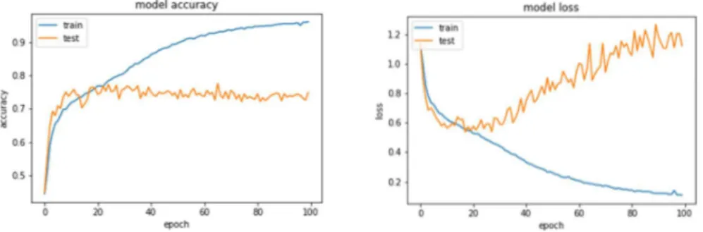
When tuning different hyperparameters in the quest for the best accuracy, one might find that the model’s accuracy is good when it comes to classifying on the data that was included in the training set, but bad at classifying data it was not trained on. This is called overfitting and occurs when the model becomes good at classifying what it has already seen but generalizes badly. Overfitting is easy to spot as the results from training the model often points to very high accuracy on the training data, but much worse on the validation. Overfitting is one of the hardest challenges to overcome when using neural networks and machine-learning classifiers[25, 26]. Some common techniques to prevent overfitting are data augmentation, meaning to modify the data within reasonable lengths (not distorting the data beyond recognition). Some augmentation techniques that are considered reasonable are cropping, rotating, flipping and zooming[27]. Other important concepts to reduce overfitting are reducing the complexity of the model and for DL adding dropout5_{. Dropout will be explained in more detail further down in}

the document. In figure 2.2 an example of overfitting is seen in a graph given from training from a CNN on the AffectNet dataset for 100 epochs. One can see that after about 20 epochs the test(validation) accuracy peaks but the training accuracy keeps improving.

Figure 2.2 - Overfitting seen in a graph given from a training session of a CNN

Underfitting is the exact opposite of overfitting and occurs when a model is unable to classify the data it was trained on and even less data it has not seen before. It is rather self-explanatory that if a model performs badly on data it has been trained on, it will not be able to make meaningful predictions on data it has not seen. Underfitting is easy to spot as the information given from training results will indicate that the accuracy is poor for both training and validation data, as well as having a very high loss. Reducing underfitting is usually easier to deal with than reducing overfitting and the most effective method to reduce it is by increasing the complexity of the model and, if possible, add more features to the input samples. In the case of dealing with images the second mentioned solution may not be possible, so the best solution might be increasing the complexity of the model.

It should be noted that in terms of interest for research, when typing the “underfitting” keyword for the IEEE Xplore digital library, one ends up with 86 hits (as of writing). But when typing the keyword “overfitting” 1682, which does imply that more research is being done in the prevention of overfitting than underfitting.

2.3.5. ML algorithms

2.3.5.1. Support vector machine

Support vector machine (SVM) is an ML algorithm mostly used for classification problems in supervised learning. Even if the mathematical process behind how an SVM performs its classification is complex, the intuition is very simple. Each input data is plotted as a point in an 𝑛-dimensional space, where 𝑛 corresponds to the number of

4_{https://developers.google.com/machine-learning/crash-course/reducing-loss/learning-rate} 5_{https://deepnotes.io/dropout}

(12)

12

deep convolutional neural networks features in your problem domain. The value of each of the features will hold a specific coordinate in this space. When all the features are plotted, a hyperplane that separates the classes is drawn to perform the classification. The training time and memory complexity increase quickly even when using a simpler form of SVM with linear kernels and the number of samples and number of features in each sample has a significant contribution to this[28]. 2.3.5.2. Linear and logistic regression

Linear regression is a basic form of regression that simply fits the best straight line between to represent the relationship between a dependent variable y and one independent variable x. One can input more than one independent variable by using multiple linear regression. Logistic regression is quite like linear regression but uses the logit function for classification[29]. In cases where more than two discrete classes, multinomial logistic regression can be used for multi-label classification problems[30]. The multi-label classification is also known as one-vs-all classification, it works by training multiple logistic regression classifiers, one for each 𝐾 classes in the problem domain. This means that when one train each of the logistic regression classifiers individually, it is trained on one class as true and all the other classes as false, hence the name one-vs-all6_.

2.3.5.3. K-nearest neighbor

K-nearest neighbor (KNN) is a lazy algorithm that utilizes a non-parametric technique when making its classification. Essentially, this means that the algorithm does not make any presumptions about the data features inputted to the model and that it does not need any training data points to generate the model. This makes KNN a strong classifier when it comes to data that one knows very little or nothing about and gives a fast training session, but a slower testing phase[31].

KNN bases the classification on feature similarity, how closely related one data point is related to another data point. 𝐾 is the number of nearest neighbors for a certain data point and the number of closest neighbors to this data point votes in what its classification outcome should be. This process is accomplished by getting the points closest to the point 𝑃 that is to be classified by creating a set 𝑆 of 𝐾 points with the shortest distance to 𝑃 based on the Euclidean distance. The majority class label present in the set 𝑆 is then set as the class for 𝑃. In the most elementary case where 𝐾 = 1, the algorithm is known as just “nearest neighbor”[31].

2.3.5.4. Naive Bayes classifier

Naive Bayes classifiers are a collection of probabilistic ML models that are based on Bayes theorem. They are highly popular to use for text classification (e.g. spam classifiers). The Bayes theorem is defined as follows:

𝑃(𝐴|𝐵) =𝑃(𝐵|𝐴)𝑃(𝐴) 𝑃(𝐵)

Using the theorem, given that 𝐵 has occurred, one can find the probability of 𝐴 happening7_{. This is what the term}

naive refers to, as the assumption is that the predictors or features are independent. Meaning that it does not correlate between say, the mouth and eyes for a happy face but looks at them both separately. There are different types of Bayes classifier that can be applied to continuous or discrete values, as well as binary or multiple class classification problems. The type that is used in this thesis work is the multinomial naive Bayes classifier for multiclass problems. Naive bayes is a very popular algorithm to apply when dealing with text classification problems, such as spam identifers[32].

2.3.5.5. Decision trees

A decision tree in ML is essentially a flowchart represented in a top-down tree to help decide with classification related problems. The bigger idea of using a decision tree is to split the dataset into smaller subsets of data until no further splits can be made and all the leaves lead to a classification of the input[33].

2.3.5.6. Random forest

Random forest is an ensemble algorithm used for classification, meaning that it consists of a group of classifiers instead of one. In the previous heading, decision trees were described and as it turns out, random forest is built up randomly created decision trees. Each prediction is made using each decision tree in the ensemble then the final prediction is based on the majority voting method. The majority voting method can be thought of as a political voting system, where each tree represents a person from a political party. When all the votes have been counted from the trees, a decision is made.

6_{https://en.wikipedia.org/wiki/Multiclass_classification} 7_{https://brilliant.org/wiki/bayes-theorem/}

(13)

13

deep convolutional neural networks The advantages of using an ensemble of decision trees instead of just one is a more robust result as it is coming from 𝑛 number of trees instead of one. It reduces overfitting since it takes the average of all prediction, canceling out biases. The ensemble can also be used for regression if needed. The disadvantages are rather straightforward, as you add more trees, you increase the complexity of the algorithm, making it slower in generating predictions. The results are not as self-explanatory as well, because in a single decision tree one can simply print a graph of the tree and follow the flowchart[33].

2.4. Deep learning

DL builds upon the concepts of ML and can be thought of as a subset to ML. The word deep can refer to the depth of a given architecture of a neural network, and while it may be debated of what classifies as deep, in general, all neural networks with an architecture that consists of more than one layer (which would be referred to as “shallow” learning) fit this category. In DL, there are many various types of neural networks that are used to solve different problems. Neural networks are particularly useful for classification or recognition problems. In the following subsections, there will be an in-depth explanation of how these types of networks are constructed and function intuitively.

2.4.1. Artificial Neural Network

Artificial Neural Networks (ANN) refers to the most typical type of DL model that consists of neurons (or nodes) layered together in layers to perform different computational tasks. Even though the networks themselves might be very complex in their nature, the nodes are remarkably simple. The nodes of an ANN are nothing but a floating-point value that is more commonly referred to as weights. These weight values are updated after each iteration through the neural network while the network is learning. The structure of a very simple ANN architecture can be seen in figure 2.3, where one layer takes the input data, passes it through two hidden layers with 4 nodes each and gives two outputs. There is no upper bound to how many layers an ANN might consist of, however, the deeper it is, the larger the solution domain to solve the specific classification problem there is. This is in many cases the desired feature and is traded off for more complexity and longer training time. Precautions should be made when deciding on the architecture for neural networks, as deeper networks might be prone to overfitting[34].

Figure 2.3 - A simple overview of an ANN architecture

When a model architecture has been decided upon, the model is initialized, and the weights are either loaded from a file or set to arbitrary values. Once the input has been given to the neural network and output has been received, the loss (rate of error) is computed for the output. Having the value of the loss function, the gradient of the chosen loss function is computed in relation to all the weights in the network. Once the value for the gradient of the loss function is acquired, this value can be used to update the model weights. This is process is known as backpropagation. Through each iteration, the values of the weights will be updated to try and move in the direction that minimizes the loss function and takes it closer to its minimum value. Next, the learning rate is used and multiplied with the gradient[34].

2.4.2. Bias

Bias is another learnable parameter, meaning it will change during training. Bias helps the network decide when a certain node activation is meaningfully activated and by how much. The bias is used right before the weighted sum is put through the activation function and is simply added to the sum of the weights. Bias essentially help the model get meaningful information from patterns that otherwise would not pass through the origin[34].

(14)

14

deep convolutional neural networks 2.4.3. Batch size

The batch size is the number of samples that are to be put through the neural network in a single pass, and we will keep taking samples until our training samples are exhausted and that will end the forward and backward pass of all the samples(epoch). In general, the larger the batch size, the quicker the model will finish through our given epochs during training. This hyperparameter is very dependent on how many samples the given machine can process in parallel through the network. The batch size is another hyperparameter set before training begins[34]. 2.4.4. CNN

CNN is a specialized type of neural network that is mainly used in the field of computer vision to solve a variety of different tasks regarding visual imagery and was introduced by Yann Lecun et al. in 1998[35]. One of the biggest reasons why CNN are showing such good performance in these types of problem is its ability to detect and identify underlying patterns that are too complex for the human eye to detect. In a CNN the input image provided is run through several hidden layers that will decompose it into features and perform a set of operations on the data. Each layer in the networks builds upon the previous layer and the output features are then used for classification[8]. There are many possible components that add properties for a CNN depending on the architecture chosen, these include but are not limited to, convolution, pooling, tangent, squashing, activation and normalization.

Figure 2.4 - An example pipeline of a CNN using images of faces as input8

CNN’s are inspired by the biology of the visual cortex, where local receptive fields represented by groups of neurons respond to a subsample of what your eyes see. Together these fields overlap each other to cover the entire field of view of the human vision. Basically, doing the actual convolution, i.e. breaking up the data received from the eyes into subsamples and processing them individually and these subsamples will reassemble a bigger and bigger picture of what you are seeing the closer you get to the final output. This makes CNN’s outstanding in performance when it comes to image classification. In this thesis work, CNN’s are used for face detection as well as image classification. An example of a CNN used for this purpose can be observed in figure 2.4 where the input are images of faces and the output is one of three classes using the SoftMax function. Another reason for using CNN’s to extract features and then classify them is that it requires a lot less computational power than a standard ANN. If one were to put the images through a standard ANN, one would first have to flatten the image into an order-1-dimensional tensor (or array if you will) where each node would correspond to a pixel value. To make an example of the number of input parameters just for one layer, a 300x300x3 image would have 270 000 parameters mapping to the input layer. With just a single hidden layer with 1000 nodes, this would make the neural network have a total of 270 million learnable parameters. This quickly gets computationally undesirable for larger architectures with more layers. CNN’s, on the other hand does not need to learn the weights corresponding to each pixel value, but instead can learn the weigh mapping to each feature layer, which will be explained in the convolution section in detail.

There are different conventions when it comes to identifying what a layer is in the DL community. In this thesis work, I will be referring to a CNN layer as the combination of a conv layer, its corresponding activation function and potential batch normalization and dropout as one layer, and pool layers as another separate layer. The subsections that follow contain further specific information on each layer’s functionality.

(15)

15

deep convolutional neural networks 2.4.4.1. Convolution

A convolutional (Conv) layer takes a tensor as input and outputs another tensor, most often in a different order than the input. An order-3 tensor is simply an image of dimensions (ℎ 𝑥 𝑤 𝑥 𝑐) where 𝑐 is the color dimension of the image. The whole dataset as input to the CNN can be regarded as an order-4 tensor where e.g.

(64 x 64 x 3 x 20) indicates that 20 RGB images of 64x64 in height and width will be used as input. Before going into a more detailed explanation of the convolution operation, it is worth noting that convolution regarding neural networks doesn’t always correspond to the operation used in pure mathematics or engineering.

In CNN’s, convolution is simply the art of breaking up the data received from images into subsamples and processing them individually and then using these subsamples as features to identify what is unique to a specific class. Provided an input image, there will exist some feature map that will act as a feature detector. In some research papers, this feature map is referred to as a kernel, this convention will be used to refer to these feature maps in this thesis work as well. An arbitrary kernel of a layer is represented as a tensor that matches the input tensor to the network, in this case, an order-3 tensor. This order-3 tensor will be smaller than the input image ℎ 𝑥 𝑤 but keep the same number of channels 𝑐 (e.g. 3x3x3 to a 300x300x3 image). All the kernels together (forming one layer) can be represented as an order-4 tensor where the fourth dimension is the number of features the layer will detect. For instance, suppose a 3x3x3x40 tensor, this means we will detect 40 features for this layer. When a tensor is inputted to a convolutional layer, the kernels are applied to the input one by one and “slide” across the input from left to right and top to bottom. This “sliding” is determined by the stride hyperparameter that gives a value of how much the kernel should move in each step. To keep the kernel from stepping out of the image bounds, one specifies the next hyperparameters padding, which can be set manually by adding 𝑛 number of rows and columns of a pre-defined number (zero is most common) around the image. This parameter can also be defined as “valid padding” which means no padding at all, or as “same padding” which means choosing a padding value so that the output size has the same ℎ𝑥𝑤 as the input size. “Same padding” is often used when one wants to avoid losing information in the conv operation, as the output will be the same in terms of height and width. The convolution operation can be observed as a visual representation in figure 2.5 for more clarity, this example can be thought of as a grayscale image of 7x7x1 with a single kernel of 3x3x1x1[36].

Figure 2.5 - A single kernel(K) applied to the input(I)

To describe the convolution operation for one layer, the following conventions will be used: padding

𝑃 ,

stride

𝑆

, filter size

𝑓

, number of kernels

𝑛 ,

where the l stands for the current layer.

With this convention, suppose we are given an

𝑛

𝑥 𝑛

input image, where ℎ, 𝑤, 𝑐 stands for height, width and number of channels respectively. Then the new height, width and, number of channels after a forward pass through the conv layer can be calculated as

𝑛

∨

=

∨

+ 1

. The new channel

𝑛

will be

equal to the number of kernels in the conv layer and each kernel in the layer will be

𝑓 𝑥 𝑓 𝑥 𝑛

and the activation 𝑎 =

𝜎

for this layer will be 𝑎 → 𝑛 𝑥 𝑛 𝑥 𝑛 . When using batch gradient descent or a vectorized implementation, the activation is 𝐴 → 𝑚 𝑥 𝑛 𝑥 𝑛 𝑥 𝑛 where m denotes the examples in the batch.

(16)

16

deep convolutional neural networks For many cases, the features that are derived from these convolutional operations by the network are not noticeable to the human eye, which is exactly why the networks are so efficient at performing classification. With enough training, they can detect theoretically anything in an image, given that enough data is provided.

When using the convolutional layers in CNN’s, one must carefully consider what convolutions to use as more kernels equal more parameters. For example, if a layer would have 128 3x3x3 kernels, this would be equals to 3x3x3x128 + the bias parameter for each kernel. In other words, 3584 learnable parameters. Notice that the number of parameters is not bound to the size of the input image, which makes CNN’s less prone to overfitting.

Regarding the choice of size for the kernels, many of the state-of-the-art CNN’s, use kernel sizes that are odd, e.g. 1x1, 3x3, 5x5, 7x7 and so on. The reason for this is debatable and is rarely discussed or given a straight answer to in the state-of-the-art literature. However, one might reason that it is because when padding (making the output the same as the input in dimensions), one is trying to avoid losing information from the image9_.

2.4.4.2. ReLU

The Rectified Linear Unit (ReLU) is not a separate layer or component of the convolutional network. It is part of the convolution process and is applied after the element-wise addition of the product of the feature map tensors has been performed with the input tensors. Before the output of the conv layer is passed forward to the next layer unit, the ReLU (non-linearity function) is applied and then the bias is added before the next forward pass is being made. ReLU can be described mathematically as:

𝑓(𝑥) = 𝑥 = max(0, x)

ReLU is arguably the most popular activation function used in CNN’s[7, 8, 37, 38]. A few reasons why ReLU has gained such influence is that firstly it is computationally cheap since it essentially is just a max function of two values[39]. Secondly, it converges fast, meaning, since its linear, it does not plateau for large values of x. Therefore, it does not experience the vanishing gradient problem that is present in other activation functions such as Sigmoid10_.

Figure 2.6 - Rectified linear function (ReLU)11 2.4.4.3. Pooling

Another layer that often is incorporated into convolutional neural networks is the pooling operation. Note that it is possible to implement this layer alongside convolutional layers, but it is by no means required to get a conv network up and running. There are several different styles pooling, in all the CNN discussed here, the max pooling operation is used. In the pooling layer there are no learnable parameters, therefore not making a compelling difference to the computational process. The pooling procedure works in a similar way to the conv layer by applying a kernel over the input tensor volumes. In figure 2.7, the max pooling operation using a 2x2 kernel applied to a 4x4 matrix can be observed. The kernel is first put in the upper left corner of the input matrix, the max value is extracted (20) and is inserted into the 2x2 output matrix. The kernel continues to move from left to right and top

9_{https://www.deeplearning.ai/deep-learning-specialization/}

10_{https://ml-cheatsheet.readthedocs.io/en/latest/activation_functions.html} 11_{https://www.tinymind.com/learn/terms/relu}

(17)

17

deep convolutional neural networks to bottom until all the maximum values are extracted and inserted into the output volume. Strides are rarely used in the pooling layer as even if we overshoot by one pixel, there will still be a maximum value in the pixels that the kernel is applied to[7, 26, 40].

Figure 2.7 - Max pooling applied to a 4x4 matrix

The max pooling operation takes an input volume of 𝑊 𝑥 𝐻 𝑥 𝐶 and requires two hyperparameters to be set before runtime, the spatial extent 𝐹𝑥𝐹 and the stride 𝑆. The operation produces an output volume of 𝑊 𝑥 𝐻 𝑥 𝐶 to be inputted to the next layer where:

𝑊 =𝑊 − 𝐹

𝑆 + 1 𝐻 =𝐻 − 𝐹

𝑆 + 1 𝐷 = 𝐷

There are two main purposes of the pooling operation, the first being helping prevent the model from over-fitting by providing as it makes an abstraction of the input volume[9]. It also reduces the input volume, hence reducing the number of learnable parameters and saving computation resources[37]. This can also be observed in figure 2.7 as the input volume of 4x4x1 outputs 2x2x1.

2.4.4.4. Flattening

After putting the input image through a CNN to extract all the features, a layer called flattening is applied to restructure an order-n tensor into an order-1 tensor(array). This layer is usually not referred to as a specific layer but a part of the fully connected layers and sometimes the fully connected layers are referred to as “hidden layers” (taken from ANNs mentioned previously)[7, 8]. This layer marks the end of the feature extraction process of the CNN and the beginning of the classification process. If the final output of the final layer in the extraction process would be a 3x3x256 tensor, one would derive some array of 2304 elements from it. From this layer and onward, the operations unique to the CNN essentially is finished and the network functions like a simple ANN that was explained in section 2.4.1.

2.4.4.5. Full connection

With the flattened array as input, one or more fully connected layers can be further applied to help the classification procedure. These layer(s) function in the exact same way as a normal ANN hidden layer, where each node in the previous layer maps to the next one and so forth. Please see section 2.4.1 for a more elaborate explanation of this. 2.4.4.6. SoftMax and cross-entropy

SoftMax in combination with cross-entropy functions as a way for the CNN’s final output to be displayed as probabilities summing up to 1. Logistic regression is closely related with SoftMax as a synonym to it is “multi-class logistic regression”, see appendix for a figure on how they relate. The SoftMax function takes an un-normalized vector as input. In the case of a neural network, this is the vector derived from the last of the fully connected layers array transposed. After applying the SoftMax function to the vector, each element 𝑖 of the vector 𝑉 will be in the interval [0,1] and the sum of the elements will be:

(18)

18

deep convolutional neural networks This vectors values can then be extracted and evaluated as they correspond the probabilities of each class predicted from the original input image. The SoftMax unit is essentially a classifier that outputs the probabilities of your classes. It works together with the entropy loss function, where SoftMax uses the gradient of the cross-entropy function to update its weights when applying stochastic gradient descent[41].

2.4.5. Transfer learning

In some cases where the problem domain is similar and/or the dataset for training is very small, transfer learning can be applied instead of constructing a new model. By using transfer learning, one can use a pre-defined model that has already been trained on a dataset and instead of retraining the model from scratch. Simply by downloading the final weights that were acquired from the training of the model and swap out the last output layer to a different classifier or a fully connected layer and SoftMax with the number of classes that you are using in your problem. If one wish to retrain some of the layers in the pre-defined architecture but not all, this can be achieved by “freezing” the layers whose weights should not be updated. Unless one has an exceptionally large dataset or a very different problem domain, it is advantageous to at least try out transfer learning before moving on to develop new models[42].

(19)

19

3. Related Work

In this section, previous works and research in FER, alongside some state-of-the-art CNN models are described and investigated in detail. The challenges and achievements of the area are covered as well.

3.1. ImageNet challenge and state-of-the-art CNN’s

Before covering separate papers regarding the specific problem of FER, a few successful state-of-the-art models using CNN’s related to object-detection and classification will be looked upon. DL and CNN’s have since 2012 to present date been winning the ImageNet challenge. The contest named the ImageNet challenge, short for Large Scale Visual Recognition Challenge (ILSVCR) is one of the largest classification competitions that evaluate algorithms for object detection and image classification in the world. According to the Stanford Vision Lab that hosts the contest, their motivation behind it is described as follows:

“One high-level motivation is to allow researchers to compare progress in detection across a wider variety of objects -- taking advantage of the quite expensive labeling effort. Another motivation is to measure the progress of computer vision for large scale image indexing for retrieval and annotation.” [43]

Alexnet is considered one of the bigger break-throughs in using CNN for image classification and entered the ImageNet competition and took first place in 2012 when the model was first introduced[44]. Alexnet is by no means a network considered to be overly complex by the standards of recent years, but nonetheless proved very powerful. Alexnet uses 11x11, 5x5 and 3x3 convolutional layers and applies max pooling, dropout and ReLU as the activation function. The architecture is built up of two pipelines making computations in parallel before connecting back together into a sequential pipeline at the dense layers and SoftMax classification. The reason for the architectures unique parallel pipeline is due to the training being processed on two Nvidia GeForce GPUs simultaneously. Moving forward two years in time (2014) the Inception V1(GoogleNet) from Google made its first appearance. It achieved a top-5 error rate very close to human level performance which even required the organizers of the challenge to evaluate. In the end, it did not beat human level performance but came very close. The architecture took inspiration from LeNet and used 1v1 convolutional layers to decrease the number of parameters while still being able to use a very deep architecture[45]. Inception has also been further improved upon in Inception v2, v3, and v4. The same year as Inception V1, VGGNet also made its debut in the ImageNet challenge. VGG uses explicitly 3x3 convolutions and utilizes lots of filters. VGG has since its appearance become widely publicly available in different variations and is frequently used for feature extraction from images. One of the major limitations of VGG is the number of trainable parameters, which is close to 138 million. Compared to Inception v1 using 4 million and was published the same year, this is quite a lot and does impact the amount of time required for training significantly[46].

While all these results are very impressive, there is one major limitation on many of the ImageNet images that are used for classification. The images that are used often contains only the object that is to be classified or at least the object that is to be classified is centered or in great focus. In real-world scenarios, this is usually not the case as the object might be obscured or there might be a lot of other objects that might be like the one to be classified. It is however understandable that the images from the dataset are given this way, as one image is related to only one specific class and not several classes, even if there are images with several objects that all are viable for classification. This problem is a fact for all tasks that build upon object detection and classification, FER included.

3.2. FER state-of-the-art

This subsection is dedicated to reviewing some related works and their approaches to the FER problem and identify successful techniques but also shortcoming in the current state-of-the-art. Furthermore, it will go into detail why FER is such a challenge task and look at how previous works have been trying to overcome these challenges. In a conference in Malaysia 2009, Adeshina, Lau [3] et al. showed their review of real-time facial expression recognition approaches. In their review, they cover extensive comparison of different approaches to both face detection and tracking, facial feature extraction and finally facial classification approaches. They concluded that most of the reported systems with high accuracy are restricted to only frontal views of the expression at a single scale. This is a challenge that has been around for some time and others have arrived at the same conclusions regarding challenges[2] to conditions in the position, poses, obstruction and illumination of the faces in images. Also, they mention that the distance from the camera has a great impact using some of the state-of-the-art detection algorithms. Furthermore, many algorithms are covered and compared for especially detection, but deep learning

(20)

20

deep convolutional neural networks and especially CNN’s are mostly covered for expression classification and not detection. They purposed that IR-images might be used to further enhance expression recognition systems in the future.

Previous research backs the fact that CNN’s outperform previous methods in classification related problems, especially in image classification problems. In 2017 Ronghe, Nakashe [6] et al. performed a hybrid architecture approach using RNN-CNN combined. In their work, the Recurrent neural network (RNN) is used in combination with the CNN to learn temporal and spectral features of emotions and to predict the subjects in the video’s emotional reactions.

Jung, Lee [37] et al. performed a comparison of DNN and CNN in 2015 and achieved impressive results with their CNN model. They used the CK+ dataset that contains 327 image sequences that include the 7 universal emotions while performing an evaluation on their CNN and DNN respectively and achieved an 86,54% recognition rate with CNN compared to a 72,78% rate on the DNN. Speculations that there is the possibility that the DNN was overfitting were taken into consideration. On top of the neural networks, they also developed a system for real-time facial detection and feature extraction. They used a Haar-like detector and then cropped the images and performed normalization before feeding them into the CNN and DNN.

In 2017, Fathallah, Abdi [47] et al. presented a new architecture network based on CNN for facial expression recognition. They evaluated and trained their model using several large public databases, such as CK+, MUG, and RAFD. The motivation behind the use of many databases is that a deep network needs a huge amount of training data, therefore, combining many databases to get a final larger one was their approach. Their approach in the CNN model used four convolutional layers where the first three are followed by max pooling layers and the last in the line is the fully connected layer. They recorded a total of 300000 iterations of the database that took 4 days to reach accuracy close to 99% in their training step. They also compared several approaches with 3, 5 and 6 layers before testing their final 8-layer structure.

Using the FERC-2013 for training, Kumar, Kumar [7] et al. applied a CNN to better predict human emotion(frame by frame) and researched how intensity changes on a face from low to high level of emotional intensity. FERC-2013 database provides 32 000 low-resolution images that are described as “emotions in the wild”, i.e taken under some changes in parameters for the images, such as distance and so on. They applied the well-studied Viola-Jones algorithm for face detection in the database set[1, 4, 15]. In their result for the detection stage, it showed the drawbacks of the Viola-Jones method when trying to detect non-frontal face images. Their final 9-layer CNN model shows a promising 90%+ accuracy on a set of seven different emotions (universal set).

Several studies point to that FER are interlinked with not only the face but also the gender and age[48-51]. Age acts on certain emotion in certain years of age, for example, children have an increase in sensitivity to all emotions from the age of 5 until adulthood, expcept for happiness and fear. Meaning that the emotions of happiness and fear are recognized much earlier than the rest in a humans life [52]. It is found that women express their emotion more intensely than men, true for both the facial expression and in a more intense mood experience. It is also stated by et al. that women express more positive emotional force than men in general.

All the above studies show an increase in accuracy when using DL for classification of the human emotion to certain facial expressions. Most of the studies are restricted to databases containing static images in controlled circumstances (e.g. CK+, JAFFE, MUG) while others provide real-time footage or in some cases databases containing video footage frames. Something to take note of is that many of the algorithms that are being used in the state-of-the-art that are published today are limited to using haar-based face detection and using grayscale datasets for training and validation. To extend the possibilities for FER this thesis work will utilize the fact that CNN has been proven to be an outstanding feature extractor in many of the works mentioned in this section of the thesis work. Further, by using deep learning for performing the detection instead of the Viola-Jones algorithm in attempts to try and overcome the restriction to detection in full frontal images only. This work also considers the use of alternative classification methods instead of the SoftMax used in many other research articles relating to FER, to try and increase the accuracy and compare these models to the SoftMax function in terms of accuracy [7, 47 ,37]. On top of these mentioned attempts on the identified challenges, the dataset that will be used will be hosting images given from “the wild” as many of the related works that have been covered only provide datasets given from controlled environments.

(21)

21

4. Problem Formulation

This thesis work is built up from several smaller problem subtasks that together form a set of research questions that have been answered or partially answered. The research questions are built around the steps that are required to implement a robust FER system and touches on the smaller sub components that make the whole system. The methods and results that are presented are based on the following research questions:

1. How well does a deep learning approach using CNN compare against the well-studied detection algorithm Viola-Jones in terms of detection accuracy and detection of faces in different orientations than full-frontal view?

2. Can different machine-learning algorithms be used to increase performance in terms of accuracy of the extracted features of a CNN in comparison to the more commonly used SoftMax function?

3. What is the difference in terms of speed and accuracy between using the different detection approaches mentioned in question 1 in combination with classification using a CNN for three emotions in real-time?

Vision based facial emotion detection using deep convolutional neural networks

M

U

S

I

,

D

E

V

,

S

Examensarbete för kandidatexamen i datavetenskap – 15 HP

Vision based facial emotion detection using deep

convolutional neural networks

Fredrik Julin

Fjn14001@student.mdh.se

Examiner: Mobyen Uddin Ahmed

Mälardalen University, Västerås, Sweden

Supervisor: Hamidur Rahman

Mälardalen University, Västerås, Sweden

Abstract

Table of Contents

1.

Introduction ... 7

2.

Background ... 8

3.

Related Work ... 19

4.

Problem Formulation ... 21

5.

Methods and Materials ... 22

6.

Results ... 29

7.

Discussion ... 38

8.

References ... 41

List of figures

List of tables

List of abbregations

AI

Artificial intelligence

FER

Facial expression recognition

ROI

Region of interest

ANN

Artificial neural network

CNN

Convolutional neural network

RNN

Recurrent neural network

DL

Deep learning

ML

Machine-learning

SVM

Support vector machine

KNN

K-nearest neighbor

1. Introduction

2. Background

2.1. Datasets

2.2. Image preprocessing

2.3. Machine learning

2.4. Deep learning

𝑃 ,

𝑆

𝑓

𝑛 ,

𝑛

𝑥 𝑛

𝑥 𝑛

𝑛

=

+ 1

𝑛

𝑓 𝑥 𝑓 𝑥 𝑛

𝜎