Prediction of training time for deep neural networks in TensorFlow

IN

DEGREE PROJECT COMPUTER ENGINEERING, FIRST CYCLE, 15 CREDITS

,

STOCKHOLM SWEDEN 2018

Prediction of training time for deep

neural networks in TensorFlow

JACOB ADLERS

GUSTAF PIHL

KTH ROYAL INSTITUTE OF TECHNOLOGY

Prediction of training time for

deep neural networks in

TensorFlow

JACOB ADLERS

GUSTAF PIHL

Bachelor in Computer Science Date: June 3, 2018

Supervisor: Stefano Markidis Examiner: Örjan Ekeberg

School of Electrical Engineering and Computer Science

Swedish title: Förutsägning av träningstider för djupa artificiella neuronnät i TensorFlow

iii

Abstract

Machine learning has gained a lot of interest over the past years and is now used extensively in various areas. Google has developed a framework called TensorFlow which simplifies the usage of machine learning without compro-mising the end result. However, it does not resolve the issue of neural network training being time consuming. The purpose of this thesis is to investigate with what accuracy training times can be predicted using TensorFlow. Essentially, how effectively one neural network in TensorFlow can be used to predict the training times of other neural networks, also in TensorFlow. In order to do this, training times for training different neural networks was collected. This data was used to create a neural network for prediction. The resulting neural network is capable of predicting training times with an average accuracy of 93.017%.

iv

Sammanfattning

Maskininlärning har fått mycket uppmärksamhet de senaste åren och används nu i stor utsträckning inom olika områden. Google har utvecklat ramverket TensorFlow som förenklar användningen av maskininlärning utan att kompro-missa slutresultatet. Det löser dock inte problemet med att det är tidskrävan-de att träna neurala nätverk. Syftet med tidskrävan-detta examensarbete är att untidskrävan-dersöka med vilken noggrannhet träningstiden kan förutsägas med TensorFlow. Allt-så, hur effektivt kan ett neuralt nätverk i TensorFlow användas för att förutsä-ga träningstiderna av andra neurala nätverk, även dessa i TensorFlow. För att göra detta samlades träningstider för olika neurala nätverk. Datan användes sedan för att skapa ett neuralt nätverk för förutsägelse. Det resulterande neu-rala nätverket kan förutsäga träningstider med en genomsnittlig noggrannhet på 93,017%.

Contents

2.2 Artificial neural networks . . . 4

2.3 Neural network training . . . 4

2.4 Deep neural networks . . . 6

2.4.1 Backpropagation . . . 6

2.4.2 The activation function . . . 7

2.5 Regression . . . 8 2.6 Overfitting . . . 8 2.7 TensorFlow . . . 9 3 Method 10 3.1 Measurement of error . . . 10 3.2 Gathering data . . . 11 3.2.1 Fixed parameters . . . 11 3.2.2 Variable parameters . . . 12 3.2.3 Collection script . . . 12 3.2.4 TensorFlow installation . . . 15

3.3 Our deep neural network . . . 15

3.3.1 Finding an accurate configuration . . . 15

3.3.2 Training and evaluation sets . . . 16

vi CONTENTS

4 Results 17

4.1 Time variation distribution . . . 17

4.1.1 An upper limit on accuracy . . . 18

4.2 Looking for patterns . . . 19

4.3 Resulting neural network . . . 21

4.3.1 Accuracy . . . 21

5 Discussion 23 5.1 Pre-processing data . . . 23

5.2 Splitting the data . . . 23

5.3 Future research . . . 24

6 Conclusion 25

Chapter 1

Introduction

Machine learning has gained a lot of interest over the past years and is now used extensively in various areas such as content filtering on social media, personalised search results, computer vision among others. One of the main approaches to machine learning consists of training artificial neural networks to produce a desired outcome. Artificial neural networks need to be trained with suitable data in order to be useful and depending on the network this process can be time consuming. The larger and more complex the network, the more time is required for training.

In 2015 the team at Google Brain released an open source machine learning framework called TensorFlow. TensorFlow simplifies some of the work that goes into creating an artificial neural network as the user does not need to implement any of the algorithms used for training. The user merely specifies the structure of the network and the data, and uses pre-written functions to start training. This simplification of the machine learning process has made the field more accessible and has lead to TensorFlow gaining popularity.

1.1 Problem Statement

Although TensorFlow simplifies the the network creation process, the training can still be time consuming. It can also be difficult to predict how long it will take to train a network, given its structure.

2 CHAPTER 1. INTRODUCTION

Our research question is, with what accuracy is it possible to create a

Ten-sorFlow model which predicts the training time of other TenTen-sorFlow models?

The models which will be investigated are deep neural networks with a single output. The model used for prediction will also be a network of the same type. The aim is for our model to produce a single output, the training time, given various parameters specifying the network to be trained.

1.2 Scope

The parameter space of possible neural network structures and computer hard-ware configurations is vast. Because of this we have limited the scope of our study in a number of ways. Firstly we have chosen to predict the training time for neural networks on a single hardware configuration. Our reason for doing so is that we only have access to a few computers, even less than the number of parameters needed to give a reasonable performance estimate. Secondly we are limiting ourselves to predicting deep neural networks with between 1 and 4 hidden layers with sizes varying between 0 and 20 nodes, and a single real valued output.

1.3 Outline

In chapter 2, machine learning theory along with a description of TensorFlow is presented. Following this, chapter 3 presents the method used in the study, which includes definitions of error and accuracy, data gathering as well as find-ing a neural network structure. The results of the study are presented in chapter 4. Lastly chapter 5 raises thoughts on the results and chapter 6 summarises the study.

Chapter 2

Background

In this chapter we present descriptions of various topics that are necessary in order to understand this thesis. This includes machine learning fundamentals as well as a brief description of the TensorFlow framework. As our study involves the use of neural networks with a single output, we have a brief section on regression as well.

2.1 Machine learning

Machine learning is a field of computer science focused on creating software that uses data to learn how to accomplish a task. Rather than following explic-itly stated rules, machine learning software looks for structure in data in order to shape its behaviour [13]. Certain tasks which may appear to be trivial, such as identifying handwritten digits, are surprisingly difficult to perform using traditional techniques. A machine learning approach can be used to perform many such tasks on an appropriate dataset [12].

2.1.1 Supervised learning

One of the two main classes of machine learning is called supervised learning. In supervised learning the data provided to the software is labelled with the desired output [4]. For example, while using machine learning to recognise

4 CHAPTER 2. BACKGROUND

handwritten digits, an image of a seven is labelled as a seven. In this way the software receives feedback determining how well it is performing so that it may adjust itself accordingly.

2.2 Artificial neural networks

Artificial neural networks (ANNs) is one form of machine learning which is based on how the human brain work. Our brain is built with neurons which are connected together. These neurons receive electrochemical signals from other neurons. Depending on the origin of the charges, their magnitude, and how the neuron is tuned it might send out a new charge to other neurons [14, 2, 18].

The equivalent of a neuron in an ANN is a node. Each node receives values from a range of inputs. The node is comprised of weights, a bias and an acti-vation function [16]. The number of weights equals the number of inputs i.e. they are mapped one weight to one input value. The output value is calculated using the activation function (a continuous mathematical function) with the sum of each input multiplied with its respective weight plus the bias as the argument [18, 8].

An ANN is, just like the brain, built with multiple nodes containing their own values for the weights and biases. It has to consist of a number of input nodes and at least one output node. Note that the input nodes are simpler in compar-ison to all other nodes since all they do is pass their value to every node in the next set of nodes. The most common way of structuring the nodes is in layers where the simplest ANN, called a single-layer ANN (see figure 2.1), has one input layer connected directly to the output layer [8].

2.3 Neural network training

In order for the output, also called prediction, of an ANN to be accurate it has to be trained. Simply put all the weights and biases have to be calibrated. There is some variation in how this can be done, however the fundamental part stays the same. First the available data is split into a set of training data and

CHAPTER 2. BACKGROUND 5

Figure 2.1: A single layer ANN [10]

a set of testing data [17, 8]. After this the weights and biases are initialised to random values. The ANN is fed with data from the training set to get a measure of how far from the correct output the prediction was. This measured error is then used to update the weights and biases after which the process is repeated until desired accuracy is reached [8].

For a single-layer ANN one approach to use is the delta rule. It includes a learning rate (a continuous value, usually, between 0 and 1), the derivative of the activation function, the input value as well as the difference between the expected output and the actual output [19]. The learning rate determines how quickly we approach a more accurate ANN. Setting the learning rate to 1 or higher introduces a risk that the learning will not converge towards the solu-tion. However, setting it too low will make the training very time consuming [8, 9].

There are different methods that vary in when and how often the weights and biases are updated. Updating the weights using only a single random datapoint from the training set each time is called stochastic gradient descent. A slower but a lot more stable version is the batch-method. It runs through the entire training dataset and uses the average of the calculated changes to update the weights only once. The last version is mini-batch, a combination of the pre-vious two, which splits the training dataset into smaller batches on which the batch method is used.

6 CHAPTER 2. BACKGROUND

Since training only gets us closer to a solution with each update we can use the same training data multiple times. This is common and therefore one complete run through the training data has been given the name epoch [8, 17].

2.4 Deep neural networks

Single layer ANNs are only able to model linear structure, therefore it is some-times necessary to introduce ANNs with layers in between the input and out-put. ANNs with multiple such hidden layers are known as deep neural net-works (DNN). Apart from these extra layers, DNNs are constructed in the same way as single layer ANNs. The output of the first layer becomes the input of the next and so on (see figure 2.2). Because the calculation of the output of each node involves a non-linear activation function, DNNs can learn non-linear structure in the data they are provided. As a result, DNNs allow for modelling of more complex structures compared to single layer networks [4]. Intuitively this is because deeper layers learn higher level features, which are combinations of the lower level features of the previous layers. For example, the first layer in a digit recognition network may learn to recognise line seg-ments, while the second combines these to recognise longer lines and loops. Finally the last layer combines these high level features to learn to recognise actual digits. Note that the hidden layers are not necessarily this understand-able, this example is only used for illustrative purposes.

Recent advances within machine learning and the increased availability of computing power (especially GPUs) have led to the field of deep learning us-ing DNNs becomus-ing increasus-ingly popular. Because of their ability to learn complex structures, DNNs are often used in areas like language modelling and computer vision [7].

2.4.1 Backpropagation

The difficult part of training a DNN was to define the error in the nodes of the hidden layer(s) in order to know how adjust their weights. This problem was solved in 1989 when back propagation was introduced. The basic idea is to work from the output layer going back one layer a time towards the input layer. In each step backwards we calculate how we want the input from each

CHAPTER 2. BACKGROUND 7

Figure 2.2: A DNN with two hidden layers [10]

of the nodes in the previous layer to change, both in what direction and by how much, with the generalised delta rule. After the values are calculated for all nodes in one layer we backpropagate and, for each node in this previous layer, sum up the value multiplied by the weight corresponding to that value. This summed up value is now the error of the node in the hidden layer and doing the same thing recursively we will eventually get back to the input layer [5].

2.4.2 The activation function

The activation function plays a significant role in training the ANN and thus also in its final accuracy. Over the past 20 years the preferred activation func-tion has changed multiple times. In chronological order some of the most popular ones are:

• Linear: '(x) = ax + b • Step function: '(x) = ( 0for x < 0 1for x 0 • Sigmoid: '(x) = 1 1+ex • ReLU: '(x) = max(0, x)

8 CHAPTER 2. BACKGROUND

2.5 Regression

The technique of creating an ANN which has a single continuous output is called regression. Regression analysis is a field within statistics focused on finding relationships between dependent and independent variables [15]. More specifically, given a dataset containing measurements of one or more indepen-dent variables and one depenindepen-dent variable, regression is used to estimate a con-tinuous function using these variables as its domain and range, respectively. For example, one might estimate a function whose inputs are the features of a car and output is the car price.

In regression analysis, an appropriate type of function is selected (guessed) beforehand and then parameterised. Subsequently, some method of measuring how well the function matches the data is selected and used to determine the optimal parameters.

2.6 Overfitting

When producing statistical models from a dataset there is a risk known as overfitting. Overfitting means that the model fits the training data very closely, but fails to accurately predict previously unseen data [11]. This phenomena can occur when the structure of the chosen model is more complex than the structure of the underlying data it is modelling. A simple example is the use of a quadratic polynomial to model a phenomena which is actually linear in nature. If the model was created from two points, the quadratic polynomial would be inaccurate for every other point except these two.

In machine learning, overfitting can occur for a number of different reasons. One common cause is training a neural network for too long. Another cause is using too many or too large hidden layers in a DNN, which can be likened to the example of using a quadratic polynomial when modelling a linear phenomena. There is also potential for overfitting when the training dataset is too small, as this will cause the ANN to learn features which may not be representative of the data in general [20].

CHAPTER 2. BACKGROUND 9

2.7 TensorFlow

TensorFlow is an open-source machine learning framework developed by the team at Google Brain. It is the successor to their previous machine learning framework DistBelief, and was developed with the intention of being more flexible. Both TensorFlow and DistBelief use dataflow graphs to represent machine learning models, but the difference is that TensorFlow takes a more general approach by having the nodes in the graph be simple mathematical operations. According to the team at Google, this encourages experimentation through its simple high-level scripting interface [1]. As such it is possible for advanced users to tailor models to suit their needs. There is also support for easily creating simple commonly used models such as regression DNNs, which is what we are using.

Chapter 3

Method

In this chapter we begin by defining the error and accuracy of our prediction DNN in order for us to be able to evaluate it. Following this we describe the process of gathering data used to train our DNN. Lastly the method used to find an accurate configuration of our DNN is presented.

3.1 Measurement of error

In order for us to get a sense of the accuracy of our DNNs predictions, it was important to choose the most relevant method of measuring its error. Initially we were using the difference between the predicted training time and the actual time to calculate an average time error. In the end we decided that a relative error would be more relevant as it is natural to care less about an error of 0.2 seconds for longer training times than it is for short ones. Because of this we decided to use the percent error defined as:

Epercent = 100·|Tactual

Tpredict|

Tactual

CHAPTER 3. METHOD 11

We define our DNNs error as the average of the percent error for all the data it is tested on: EDN N = 1 n n X i=1 E_percenti

Where n is the number of test entries and Ei

percentis the percent error for test

entry i. Given this error, we define the accuracy of our DNN as: ADN N = 100 EDN N

3.2 Gathering data

Our approach to creating a DNN capable of predicting training times begins with gathering data. In order to provide useful predictions, the DNN we create needs data to be trained with. We have chosen to represent this data in the form of a list of parameters specifying the configuration of a DNN, along with the time it took to train it. The specific configurations measured along with how the measuring was done is presented in greater detail below.

3.2.1 Fixed parameters

There were a number of parameters which remained the same for all the train-ing sessions we ran. The activation function we used is ReLU. The method of backpropagation used in TensorFlow by default is Adagrad which is a vari-ation of gradient descent [3]. In addition the hardware specificvari-ations of the machine doing the training were:

• OS: Ubuntu 16.04 LTS

• Processor: Intel Core i5-3210M 2.5GHz • Memory: 8GB DDR3 1600 MHz

12 CHAPTER 3. METHOD

3.2.2 Variable parameters

As previously described there are multiple parameters that make up the struc-ture of an ANN. Here we present the parameters which were varied when gath-ering our data. A set of these parameters is referred to as a DNN configuration in this thesis. To make the project feasible we have chosen to only look at a subset of the possible parameters which we think are interesting.

• Steps: The number of times the DNN updates all weight and bias values using one batch of data.

• Batch size: The number of data points used for each step.

• Input nodes: The number of nodes in the input layer. This is essentially the number of features we are using from the underlying data when train-ing. As such it is limited by the total number of features available in the data.

• Layer structure: A list of integers with each integer specifying the num-ber of nodes in the hidden layer with this index.

3.2.3 Collection script

In order for our DNN to be able to learn how the various parameters influence the training time, we had to gather data by varying the parameters extensively. To simplify the data gathering we created a python script. We defined constant values in lists for each of the parameters we wanted data for. Each list contains at least three values representing the values that the parameter will take. For all possible permutations of parameters the script records the time it took to train the DNN. The resulting training time together with the parameters is saved to a file in CSV format.

We noticed a variation in the training time when using the same parame-ters multiple times. Because of this the script also includes the possibility of recording training times for the same parameter permutation multiple times. In the first version of the script we included TensorFlow in the collection script and had a function which created and trained a DNN. We noticed that memory

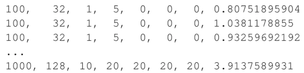
CHAPTER 3. METHOD 13 100, 32, 1, 5, 0, 0, 0, 0.80751895904 100, 32, 1, 5, 0, 0, 0, 1.0381178855 100, 32, 1, 5, 0, 0, 0, 0.93259692192 ... 1000, 128, 10, 20, 20, 20, 20, 3.9137589931

Figure 3.1: Excerpt from output of running the collection script. From left the values represent: steps, batch size, input layers, number of nodes in first hidden layer, nodes layer 2, nodes layer 3, nodes layer 4, time taken.

usage would continue to increase while the script was running. Our assump-tion is that this behaviour was caused by TensorFlow keeping record of the training made in memory. In order to fix this we moved the former function into a new python script which outputs the training time. This script is then called from our main collection script as a sub-process from which the time taken is recorded. The new approach increases the time needed for collecting the same amount of data since python and TensorFlow needs to start over for each permutation. However, this more closely resembles training done for real and should thus yield more accurate data.

Generating permutations

Here we present values we used for each parameter when generating permuta-tions. The values in the lists represent the possible values that the correspond-ing parameter can take.

• steps = [100, 500, 1000] • batch_size = [32, 64, 128] • input_nodes = [1, 5, 10]

• layer_structures = [[5, 0, 0, 0], ...]

The lists in layer_structures will contain all the possible hidden layer structures with between 1 and 4 layers where each layer has either 5, 10 or 20 nodes. An element in the layer_structures list will always be a list of

14 CHAPTER 3. METHOD

four values since we are restricted by the fact that our DNN is required to have a fixed number of input values. It would be interesting to test with more hidden layers but the time taken for collecting data would be outside of the scope of this study.

An excerpt from collect.py:

# Record t h e t r a i n i n g t i m e f o r each p e r m u t a t i o n # o f p ar ameter s aka c o n f i g u r a t i o n for s in s t e p s : for b in b a t c h _ s i z e : for i in i n p u t _ n o d e s : for l in l a y e r _ s t r u c t u r e s : for r in range (RUNS ) :

recordTime ( s , b , i , l ) def recordTime ( s , b , i , l ) : c o n f i g = [ s , b , i ] + l c o n f i g _ s t r i n g = l i s t (map( str , c o n f i g ) ) bashCommand = [ " python " , " d n n _ r e g r e s s i o n . py " ] bashCommand += c o n f i g _ s t r i n g t i m e _ t a k e n = f l o a t ( s u b p r o c e s s . c h e c k _ o u t p u t ( bashCommand ) ) c o n f i g += [ t i m e _ t a k e n ] o u t _ s t r i n g = " " for p in c o n f i g : o u t _ s t r i n g += s t r ( p ) + " , " # Remove t r a i l i n g " , " o u t _ s t r i n g = o u t _ s t r i n g [: 2] print ( o u t _ s t r i n g ) Dummy model

The model used when gathering training time data in the collection script is one which is included in the TensorFlow repository. It is a regression model

CHAPTER 3. METHOD 15

which tries to predict the price of a car given some information about it such as horsepower, engine size, highway mph etc. It also comes bundled with a dataset including 149 labelled entries. We have slightly changed the model in order for us to be able to set the variable parameters using the permutations from our script.

3.2.4 TensorFlow installation

When installing TensorFlow, there are some different possibilities available. You can either install pre-built TensorFlow binaries or build it from source. We decided to build TensorFlow from source, and followed the instructions provided on the TensorFlow website. The only variable stage of building is when running a configuration script. The script allows the user to enable specialised features such as GPU and JIT support. By answering a number of yes/no questions the user decides which features to enable. We answered these questions in the same way as they were answered in the instructions [6]. There were also a number of questions when we ran it which were not in the instructions. We answered no to all of these questions.

3.3 Our deep neural network

After the collection of data on training times we needed to configure our DNN which would perform the actual prediction. This includes determining the hidden layer structure, number of steps and batch size leading to an accurate DNN.

3.3.1 Finding an accurate configuration

There is an infinite number of possible configurations. Because of this we needed a method for automating the search. We started out by manually test-ing different configurations and trytest-ing to find a pattern for which ones had higher accuracy in comparison to others. We quickly realised that it would be much less tedious if we automated the process. By modifying the collection script we had used for gathering data, we were able to create a new script for

16 CHAPTER 3. METHOD

this purpose. The new script trains and tests DNNs with different configura-tions and records their accuracies in a separate file. The script explores all the possible structures using between 1 and 5 hidden layers, where each layer can contain either 10, 20 or 30 nodes. For each structure the number of steps varies between 5000 and 25000 by increments of 5000. The batch size remains fixed.

3.3.2 Training and evaluation sets

In our case, shuffling the gathered data before splitting it into a training and evaluation set would yield erroneous results. No data used for evaluating should ever have been seen during training since the goal of the DNN is to make predictions for previously unseen data. Because we have more than one training time recorded per configuration, shuffling them all would most likely lead to the training and evaluation sets both having data on the same con-figuration. Therefore, what should be done is to group data with the same configuration before splitting.

Since how the data is split affects the results of training it is of essence to be able to easily split the data. Hence, we created a script that groups all data with the same configuration. It then shuffles and lastly splits configurations in two parts containing 70% and 30% of the data. The set with 70% of data is used for training and the other for evaluation.

Chapter 4

Results

In this chapter we begin by describing the discovery of an upper limit on the accuracy of a prediction DNN. Following this we describe the process of in-vestigating if there is a correlation between the hidden layer structures and accuracy of a DNN. Lastly we present the most accurate DNN we found.

4.1 Time variation distribution

As previously mentioned in section 3.2.3 we noticed that there was some vari-ance when training the same DNN multiple times. For example, when training a neural net with one hidden layer of size five and one input node for 100 steps, we recorded a variety of times ranging from around 0.808 to 1.04 seconds (see figure 3.1). As a result of this discovery we decided to train each configuration 25 times, in the hope that our DNN would have a better possibility of learning the expected value.

In order to better understand this variation we decided to look at the probability distribution underlying it. Using one DNN configuration we first calculated its mean time with the 25 recorded times. Following this we calculated the percent time deviation of each of the 25 recorded times with respect to the mean.

18 CHAPTER 4. RESULTS

Figure 4.1: Time variation plot

D_percenti = ti Tmean Tmean where Tmean = 1 25 25 X i=1 ti Di

percent is the percent deviation of the ith time recorded from the mean time.

We proceeded to do this for each DNN configuration we had gathered data on and created a frequency plot from the results. As we can see from the plot in figure 4.1, the percent time deviation from the expected value appears to come from a normal distribution.

4.1.1 An upper limit on accuracy

As the most probable value for a certain configuration is the expected value, an optimal DNN should always predict this value. Because the variance in figure 4.1 is not 0, even an optimal DNN would not have an error of 0%. If an optimal DNN would be tested using an infinite amount of data, the average error would equal the average absolute deviation (AAD) of the distribution

CHAPTER 4. RESULTS 19

which figure 4.1 approximates.

AAD = 1 n n X i=1 |Dpercenti |

The reason this is important is because one cannot reasonably expect the error of our DNN to be lower than the AAD. Our calculation of the AAD, based on our limited data collection, turned out to be:

AAD = 2.535% Thus an upper limit on the accuracy of our DNN is:

Alim = 100 AAD = 100 2.535 = 97.465%

4.2 Looking for patterns

As mentioned in the method section, we created a script to find an accurate DNN configuration. One might expect there to be some kind of pattern de-termining whether a particular hidden layer structure performed well or not. With this expectation we examined the data collected by the script in order to look for such a pattern. As it is difficult to parse several thousand lines of data in text form, we realised we would need to take a more visual approach. One thing we had noticed while looking at the data is that some similar hidden layer structures (one layer differing by 10 nodes) had very different accuracies (up to 30% difference). Because of this we wanted to see if this was just an anomaly, or if it applied more generally to the data. This lead to the creation of a graph of pairwise distances between structures and their accuracy. The graph was created by going through each possible structure pair in the data. Their 5-dimensional structure distance as well as their 1-dimensional distance in accuracy was plotted as points in the XY-plane.

20 CHAPTER 4. RESULTS

Figure 4.2: Looking for patterns between structure and accuracy

Let Zlayer = [z1, z2, z3, z4, z5] be a hidden layer structure and Zacc its

accu-racy. Then the point for the pair of structures (A, B) would have the following coordinates:

x =p(a1 b1)2+ (a2 b2)2 + (a3 b3)2+ (a4 b4)2+ (a5 b5)2

y =_|Aacc Bacc|

The resulting graph seen in figure 4.2 reveals that there is no correlation be-tween structure distance and accuracy distance. If there had been a correlation, the points in the graph should have been closer to resembling samples from some increasing function. However, regardless of which structure distance one examines there are points spanning the whole range of accuracy distances. As such there appears to be no simple pattern for determining which hidden layer structures are good and which are not.

CHAPTER 4. RESULTS 21

4.3 Resulting neural network

Without knowing the reason why a certain hidden layer structure is better than another we decided to simply select the most accurate configuration produced by the script from section 3.3.1. We ran the script twice and calculated the average accuracies for all the configurations. The most accurate configuration is listed below. • layers: [30, 30, 20, 10, 20] • batch: 100 • steps: 25000 • accuracy: 96,50847%

4.3.1 Accuracy

When evaluating the resulting configuration multiple times, shuffling and split-ting the data each time, we discovered that its accuracy varied between 65% and 97%. While experimenting with the batch size and steps we noticed that decreasing the batch size to 10 and increasing the steps to 50000 produced a more accurate DNN.

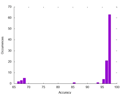
Because of the varying accuracy we decided to train and evaluate the config-uration 100 times, again shuffling and splitting the data each time. In order to get a better understanding of the data gathered, we created a frequency plot (see figure 4.3). The plot reveals that most of the accuracies are clustered around either 67% or 96%.

The resulting accuracies can be summarised as follows: • Max: 96.590%

• Average: 93.017% • Min: 65,434%

22 CHAPTER 4. RESULTS

Chapter 5

Discussion

In this chapter we present different thoughts that occurred to us while conduct-ing the study. Finally we present some ideas for future research related to our study.

5.1 Pre-processing data

Our intuition lead us to believe our DNN should learn the expected value when training. If this is what it actually learns is difficult, if not impossible, to an-swer. One way of making sure the expected value is learned is to pre-process the data used for training. We could have calculated the average training time for each of the configurations used instead of relying on the DNN to learn from all the data.

5.2 Splitting the data

When testing what we thought was the best configuration possible we noticed the accuracy fluctuating drastically. Since the only thing we changed in be-tween evaluations was the split, we could easily conclude it was the cause of the fluctuation. What stood out the most was how divided the accuracy was. Most of the time it was around 96% but occasionally and consistently it rose

24 CHAPTER 5. DISCUSSION

to slightly below 70%. There is only one reason we could come up with as an explanation. The reason is that the split is done is such a way that the config-urations in the training and test sets are very different, leading to an overfitted DNN. However, this seems highly unlikely given that we have 3240 different parameter sets which are split 70/30.

5.3 Future research

Because of the limited scope of this study, the types of DNNs we predict the training times of are limited in kind, size and steps trained. In order for this research to be of any practical use it would be necessary to produce a more generalised training time predictor. This study provides some evidence that it is indeed possible to produce accurate predictions of training times using DNN regression, and thus can serve as justification for more extensive research in the future. Disregarding the actual DNN being predicted, one of the most lacking aspects of our study is the exclusion of computer specifications as pa-rameters in the DNN. Another limitation of our study is the fact that we are only predicting times for training up to 1000 steps. All these limitations mean that there is a large number of paths to explore for future research.

Some suggestions for future research are: • parameters for computer specifications • more hidden layers

• larger hidden layers • different types of layers • multivariate outputs • more training steps

Chapter 6

Conclusion

In this study we investigated the ability to accurately predict training times for deep neural networks. Both the feasibility of creating a predictor and with what accuracy one could be made. Training times were recorded using multiple different configurations of a DNN. Analysing the recorded training times we discovered a theoretical upper limit on the accuracy. For our data this turned out to be 97.465%. These training times were also used for training and testing in order to find an accurate predictor in the form of a regression DNN. The most accurate regression DNN we found is capable of predicting training times with an average accuracy of 93.017%. Although, most predictions have around 95% accuracy.

Bibliography

[1] Martin Abadi et al. “TensorFlow: A system for large-scale machine learning”. In: 12th USENIX Symposium on Operating Systems Design

and Implementation (OSDI 16). 2016, pp. 265–283. : https:// www.usenix.org/system/files/conference/osdi16/ osdi16-abadi.pdf.

[2] Konstantin V Baev. Biological Neural Networks: Hierarchical Concept

of Brain Function. eng. 1998. : 1-4612-4100-6.

[3] John Duchi, Elad Hazan, and Yoram Singer. “Adaptive Subgradient Methods for Online Learning and Stochastic Optimization”. In: J. Mach.

Learn. Res. 12 (July 2011), pp. 2121–2159. : 1532-4435. : http: //dl.acm.org/citation.cfm?id=1953048.2021068. [4] Aurélien Géron. Hands-On Machine Learning with Scikit-Learn and

Tensorflow. eng. 2017. : 9781491962299.

[5] Ian Goodfellow, Yoshua Bengio, and Aaron Courville. Deep Learning. http://www.deeplearningbook.org. MIT Press, 2016. [6] Installing TensorFlow from Sources. Apr. 2018. : https://www.

tensorflow.org/install/install_ sources (visited on

04/23/2018).

[7] Alexandros Karatzoglou and Balázs Hidasi. “Deep Learning for Rec-ommender Systems”. In: Proceedings of the Eleventh ACM Conference

on Recommender Systems. RecSys ’17. Como, Italy: ACM, 2017, pp. 396–

397. : 978-1-4503-4652-8. : 10.1145/3109859.3109933. : http : / / doi . acm . org . focus . lib . kth . se / 10 . 1145/3109859.3109933.

[8] Phil Kim. MATLAB Deep Learning With Machine Learning, Neural

Networks and Artificial Intelligence. eng. 2017. : 1-4842-2845-6.

BIBLIOGRAPHY 27

[9] S. Knerr, L. Personnaz, and G. Dreyfus. “Single-layer learning revis-ited: a stepwise procedure for building and training a neural network”. In: Neurocomputing. Ed. by Françoise Fogelman Soulié and Jeanny Hérault. Berlin, Heidelberg: Springer Berlin Heidelberg, 1990, pp. 41– 50. : 978-3-642-76153-9.

[10] Michael A. Nielsen. Neural Networks and Deep Learning. http:// neuralnetworksanddeeplearning.com/. Determination Press, 2015.

[11] overfitting. In: Oxford living dictionaries. Oxford University Press, 2018. : https://en.oxforddictionaries.com/definition/ overfitting(visited on 2018).

[12] Md Jubaer Hossain Pantho, Festus Hategekimana, and Christophe Bobda. “A System on FPGA for Fast Handwritten Digit Recognition in Embed-ded Smart Cameras”. In: Proceedings of the 11th International

Confer-ence on Distributed Smart Cameras. ICDSC 2017. Stanford, CA, USA:

ACM, 2017, pp. 35–40. : 978-1-4503-5487-5. : 10.1145/

3131885.3131927. : http://doi.acm.org.focus.

lib.kth.se/10.1145/3131885.3131927.

[13] Gunnar Rätsch. “A Brief Introduction into Machine Learning”. eng. In: (2004).

[14] Raúl Rojas. Neural Networks A Systematic Introduction. eng. 1996. : 3-642-61068-4.

[15] Ali S. Hadi Samprit Chatterjee. Regression Analysis by Example 5th

Edition. eng. 2012. : 0470905840.

[16] Subana Shanmuganathan. “Artificial Neural Network Modelling: An Introduction”. In: Artificial Neural Network Modelling. Ed. by Subana Shanmuganathan and Sandhya Samarasinghe. Cham: Springer Interna-tional Publishing, 2016, pp. 1–14. : 978-3-319-28495-8. : 10.

1007/978-3-319-28495-8_1. : https://doi.org/

10.1007/978-3-319-28495-8_1.

[17] Ivan Nunes da Silva et al. “Artificial Neural Network Architectures and Training Processes”. In: Artificial Neural Networks : A Practical

Course. Cham: Springer International Publishing, 2017, pp. 21–28. :

978-3-319-43162-8. : 10.1007/978-3-319-43162-8_2.

: https://doi.org/10.1007/978- 3- 319- 43162-8_2.

28 BIBLIOGRAPHY

[18] Ivan Nunes da Silva et al. “Introduction”. In: Artificial Neural Networks

: A Practical Course. Cham: Springer International Publishing, 2017,

pp. 3–19. : 978-3-319-43162-8. :

10.1007/978-3-319-43162- 8_ 1. : https://doi.org/10.1007/978-

3-319-43162-8_1.

[19] Ivan Nunes da Silva et al. “The ADALINE Network and Delta Rule”. In: Artificial Neural Networks : A Practical Course. Cham: Springer International Publishing, 2017, pp. 41–54. : 978-3-319-43162-8.

: 10.1007/978-3-319-43162-8_4. : https://doi.

org/10.1007/978-3-319-43162-8_4.

[20] Nitish Srivastava et al. “Dropout: A Simple Way to Prevent Neural Net-works from Overfitting”. In: J. Mach. Learn. Res. 15.1 (Jan. 2014), pp. 1929–1958. : 1532-4435. : http : / / dl . acm . org . focus.lib.kth.se/citation.cfm?id=2627435.2670313.