Using Maximum Coverage to Optimize Recommendation
Systems in E-Commerce
∗Mikael Hammar
Apptus Technologies Trollebergsvägen 5 SE-222 29 Lund, Sweden
mikael.hammar@apptus.com
Robin Karlsson
Apptus Technologies Trollebergsvägen 5 SE-222 29 Lund, Sweden
robin.karlsson@apptus.com
Bengt J. Nilsson
Dept. of Computer Science Malmö University SE-205 06 Malmö, Sweden
bengt.nilsson.TS@mah.se
ABSTRACT
We study the problem of optimizing recommendation sys-tems for e-commerce sites. We consider in particular a com-binatorial solution to this optimization based on the well known Maximum Coverage problem that asks for the k sets (products) that cover the most elements from a ground set (consumers). This formulation provides an abstract model for what k products should be recommended to maximize the probability of consumer purchase. Unfortunately, Max-imum Coverage is NP-complete but an efficient approxima-tion algorithm exists based on the Greedy methodology. We exhibit test results from the Greedy method on real data sets showing 3–8% increase in sales using the Maximum Cov-erage optimization method in comparison to the standard best-seller list. A secondary effect that our Greedy algo-rithm exhibits on the tested data is increased diversification in presented products over the best-seller list.
Categories and Subject Descriptors
H.3.3 [Information Storage and Retrieval]: Informa-tion Search and Retrieval—InformaInforma-tion filtering, Retrieval models, Search process
Keywords
Recommendation systems; e-Commerce; Optimization; Max-imum Coverage
1.
INTRODUCTION
Consider an e-commerce site selling products to potential customers. The aim of the e-commerce marketer is to maxi-mize the profit of the site. From the consumer’s perspective, the process of purchasing a product on a site can consist of a general search on a search engine to find the site, followed by ∗This research is part of the project “Self Learning Op-timization Systems for Electronic Commerce” funded by a grant from the Swedish VINNOVA innovation agency; see http://www.vinnova.se/en/.
Permission to make digital or hard copies of all or part of this work for personal or classroom use is granted without fee provided that copies are not made or distributed for profit or commercial advantage and that copies bear this notice and the full citation on the first page. Copyrights for components of this work owned by others than the author(s) must be honored. Abstracting with credit is permitted. To copy otherwise, or republish, to post on servers or to redistribute to lists, requires prior specific permission and/or a fee. Request permissions from permissions@acm.org.
RecSys’13,October 12–16, 2013, Hong Kong, China.
Copyright is held by the owner/author(s). Publication rights licensed to ACM. ACM 978-1-4503-2409-0/13/10 ...$15.00.
http://dx.doi.org/10.1145/2507157.2507169
further searches and browsing on the site to find the product and conclude the purchase.
In fact, we consider searches to be just one aspect of more general searching schemes, denoted navigation. Navigation strategies where the customers probe the site to try to reach a loosely specified goal in several steps are called associative searches. A solution to associative search needs to let the customers explore the site to achieve a possibly undefined search goal. In contrast, a deterministic search is performed to reach a specific search goal, a purchase, already known to the customer. We therefore differentiate between customers doing associative search and deterministic search and call them associative customers and deterministic customers re-spectively.
The associative customer is a potential but uncertain buying customer, and it is the marketer’s responsibility to ensure that the customer buys something. A common strategy is to provide recommendations based on the customer’s navi-gation history and knowledge about the sales history of the site. The navigation history provides a selection of the prod-uct catalogue but this may still be much too large to be presented to the customer. Therefore, a small number of products, we denote this number k, have to be selected to be presented to the customer. In reality, many e-commerce sites present the k most popular products, i.e., the products with the highest sales, possibly weighted with profit margin or product type, the so-called best-seller list. The best-seller list is a natural choice for recommendations. The underlying assumption is that, in the short term, the sales history of the site is an accurate model for the future sales distribution. Our main insight is that, instead of optimizing on popular-ity, one should maximize the probability that a customer makes a purchase. We show that this, together with some natural design changes to the e-commerce site, will increase total sales. For a marketer, it is important to make the customer purchase something as early as possible. The cus-tomer life-time value is optimized by other means, such as product recommendations or targeted campaigns once more information about the customer is available. This strategy leads to presenting a different set of products than the best-seller list. Just presenting the most popular products is not the best strategy since several of the products on the best-seller list may be products that are commonly purchased together. In this case, it is beneficial to present other
prod-ucts that have lower sales but attract more varied consumer groups.
The problem of finding the k items from a product list that maximizes the probability of a purchase is a well-known com-putational problem called Maximum k-Coverage, a variant of the famous Set Cover problem [9, 14]. A greedy algorithm can be used to efficiently approximate a solution [5, 13, 19]. We can make additional recommendations to the customer using data associated to each product that was listed. We call such recommendations product associated recommenda-tions. In marketing terms they are known as “Those who bought this also bought. . . ” or “Those who viewed this bought. . . ”. Product associated recommendations can be implemented efficiently using common graph algorithms [6]. Our aim is to illustrate how the maximum coverage list in conjunction with product associated recommendations im-proves on the standard practice to use the best-seller list, even if these are taken together with product associated rec-ommendations. We perform several experiments on real e-commerce data to show that the greedy algorithm together with product associated recommendations significantly out-performs the best-seller list, even with product associated recommendations.
The implication of our research is that the e-commerce site needs to 1) apply the maximum coverage algorithm while the user is interacting with the site, and 2) apply product recommendations as easily and naturally as possible during the user’s interaction with the site. The first implication means that every interaction with the site should be opti-mized towards converting the customer rather than selling a particular product. This view is customer centric rather than product centered. The second implication is the key towards what we call natural browsing. A site that applies this recommendation methodology makes sure that recom-mendations are available on every page, not just hidden on product pages.
The paper is organized as follows. In the next section, we present the details of our experimental setup. Section 3 shows empirically that the Greedy algorithm produces the optimal maximum coverage list in almost every case and, in the few cases that it does not, it produces a list that covers 99% of the optimal list, thus significantly beating the guar-anteed approximation ratio of 63%. Section 4 presents the results from our experiments and in Section 5, we show that the maximum coverage list also improves on the diversifica-tion of the presented products in reladiversifica-tion to the best-seller list. In Section 6 we discuss the significance of our results. In Section 7, we give a suggestion of how to adjust a site to exploit our results to further improve the sales figures. In Section 8, we discuss future research and possible extensions.
2.
METHOD
2.1
Best-Seller and Maximum Coverage Lists
Let us look at the first step of the sales process separately, to maximize the probability that a customer makes a purchase. We assume that the marketer has data about previous sales. Given the current navigation selection, what choice of
prod-ucts should the marketer present on the site? The most
common method is to present the currently most popular products, often in a best-seller list displaying the k products with the highest number of purchases. The ambition with this scheme is to attract future customers to the products of the site. This method is easy to understand and simple to compute, even dynamically, in O(kn) time, where n is the number of products in the current product selection. We call it the B-list (short for best-seller list ).
However, this tentative solution does not take into account that several best-selling products can appeal to the same group of customers. The marketer can be better off present-ing products that sell slightly less than those in the B-list but spread across larger groups of customers. To achieve this, we want our list to appeal to as many different types of customers as possible. We look at recent sales data as a probability distribution of sales over the product selection and find, for an arbitrary customer, the k products maximiz-ing the probability that the customer makes a purchase from these k products. With knowledge of what previous cus-tomers have bought, we have additional information about dependencies between products and we can make use of this knowledge. Let us formalize this and let U = {u1, . . . , um}, be the customers that previously have bought products and let F = {S1, . . . , Sn} denote the products in the product selection. If we associate the customers that have purchased product Si, we can view Sias a set of those customers. The family F represents the products, where uj is in Si if and only if customer uj has bought product Si. Our objective now is to establish the k sets F∗ = {Si1, . . . , Sik} that
to-gether contain as many different customers uj as possible. This is a well-known problem from Combinatorial Optimiza-tion denoted the Maximum k-Coverage problem and is for-mally defined as follows:
Name: Maximum k-Coverage
Instance: A universe of elements U = {u1, . . . , um}, an integer value k and a family of sets F = {S1, . . . , Sn}, where each set Siis a subset of U . Objective: Find a subfamily F∗⊆ F such that |F∗| ≤ k and the number of covered elements |S
S∈F∗S| is maximised, i.e. using up to k sets,
cover as many elements as possible.
The maximum coverage problem is a variant of the set cover problem and these problems are well researched [2, 3, 5, 11, 12, 13, 18, 19, 20]. Unfortunately, these are NP-hard prob-lems [9, 14], and thus we cannot expect to optimally solve them efficiently. However, using a simple greedy algorithm (as shown in Algorithm 1), we can achieve an approximate solution for maximum coverage that is guaranteed to have an approximation ratio of (e − 1)/e ≈ 0.6321, where e is the base of the natural logarithm, so the greedy algorithm will always cover at least 63% of the maximum possible number of customers that can be covered, and it can be shown that this is essentially as good as can be achieved with a polyno-mial time approximation algorithm [7]. This algorithm can be implemented to run in O(k ·P
S∈F|S|) ⊆ O(knm) time. We denote the list of k products produced by the greedy algorithm, the M-list (short for Maximum Coverage list ).
2.2
Ageing
One very important aspect to consider is how to deal with older sales in relation to newer ones. Since recent sales data
Algorithm 1 GREEDY-MAX-COVERAGE(U , k, F ) 1: R ← U 2: F∗← ∅ 3: for i from 1 to k do 4: S ← maxS∈(F \F∗)|S ∩ R| 5: F∗← F∗∪ {S} 6: R ← R \ S 7: if |R| = 0 then break 8: return F∗
will say more about what products are popular at the mo-ment than old data, some kind of ageing model is needed to make older sales have less impact than more recent ones. A time-based window, that forgets sales data as they turn older than some time t, is perhaps the easiest and most intu-itive kind of model. Another approach is the session-based window, that always keeps the same number of sessions in the sales data. This window will keep the amount of data constant even if the rate of sales on the site changes. More advanced models can gradually decrease the importance of sales with time [17]. No matter what model is used, a long window is slow to catch on to trends and tends to show prod-ucts that are less trend sensitive. A short window catches trends faster but is more sensitive to noise due to lack of data. One such kind of noise is customers that purchase several copies of the same product. This spike in sales could push an otherwise unremarkable product to the top of the B-list. An easy way to avoid this unwanted effect is to order products by the number of customers that have bought the product, rather than the product’s total number of sales.
2.3
Product Associated Recommendations
When the customer reaches the product page on the way to make a purchase, it is customary to show some kind of recommendations based on the product viewed (and some-times also based on knowledge about the customer). Popular methods are “Those who bought this also bought. . . ” (de-noted BB) and “Those who viewed this bought. . . ” (de(de-noted VB) or variations thereof. In many cases, such recommenda-tions can also be presented in earlier phases of the navigation and not only when the customer reaches the product page. We denote recommendations that depend on given products (and possibly other information) product associated recom-mendations or PARs and in the second step of our strategy, we use PARs to further enhance the total recommendations of the e-commerce site.
PARs can be implemented efficiently using common graph algorithms [6]. We maintain a weighted graph where each product in the product catalogue is a node and whenever two products are purchased together (in the case of BB), we increase the weight between the corresponding nodes. For other variants of PAR methods, similar strategies can be implemented.
2.4
Motivation
As we will see, (BB) PARs complement Maximum Coverage as a product S that has sold well but is not on the M-list is very likely to be picked as a PAR for something else on the M-list. The reason for this is that the M-list contains a
product S0 that is likely to be bought in conjunction with S, and hence, S is a PAR of S0.
In contrast, PARs do not complement the B-list as well. The reason for this is that if a product S0 is in the B-list, and has an associated PAR S that has sold well, it is likely that S will also be in the best-seller list. Thus, the products on the best-seller list will, in many cases, be in each other’s recommendations.
The M-list effectively presents the products that maximize the probability of a purchase, whereas the B-list simply presents the most popular products. Our experiments will show that by presenting the M-list instead of the B-list dur-ing browsdur-ing, and, in the same context, present related just-in-time product recommendations, the user is confronted with all the benefits of the M-list but also with the most popular products of the B-list available via recommenda-tions. Hence, product associated recommendations together with the M-list give us the best of both maximizing the prob-ability of sales and also showing the most popular products.
2.5
The Experiments
We make two types of experiments on data from two real
e-commerce sites. The two sites are a book store and a
hardware store (selling DIY material). The first experiment compares the greedy method to the optimal solution to the maximum coverage problem on data from our sites. The results of this experiment are presented in Section 3. The second and main type of experiment aims to compare the effect on sales between the M-list and the B-list, together with PARs. This can be done with live evaluations such as A/B tests, where the users would be split in two groups and each group is shown a different alternative. However, live testing requires control over what is shown on a website and can be costly if one strategy performs significantly worse than the other strategy. Instead, we evaluate the two strate-gies using logged sales data. This problem of evaluating a new behavior, or policy, using only observations collected during the execution of another policy is known as policy evaluation [15].
To simplify our experiments, we compare the M-list and B-list with PARs as they would appear on the sites’ top pages but we are confident that our method works equally well under the general situation that the customer navigates through the site, dynamically changing the part of the prod-uct catalogue currently considered by the recommendation system.
The data available for the experiments is a sequence of ses-sions where each session contains a time, a customer ID and a list of purchased products. The data contains the complete sales information of the book store (116 000 sessions) and the hardware store (28 000 sessions) during 60 days. We use the data from the first 30 days as “warm-up” data to stabi-lize the results of the algorithms. The result we present are from runs of the algorithms on the last 30 days, as follows:
• Data A: 30 days of sales data from a book store. • Data B: 30 days of sales data from a hardware store.
Our evaluation method is to go through the recorded sales data in chronological order and update the different lists according to the data seen so far. Then the different lists are scored as follows:
• For each session, give a list one product point for each product sold that is in the list at the time of the trans-action.
• For each session, give a list one session point if the list shows any of the products purchased in the session at the time of the transaction.
These two different scores correspond to the two different types of lists we want to evaluate. Essentially, the B-list tries to optimize product points and the M-list tries to optimize session points.
In order to measure the effect of PARs on a list we also con-struct an associated set of PARs in the following way: For each product in the list take the top three BB PARs for the product and put them in a PAR set. As two products could both recommend the same product any duplicates are re-moved, also any product in the original list is removed from the PAR set. We keep the number of PARs considered for each product low since, in reality, a large number of product associated recommendations would not be considered by a customer.
Our way of measuring using session points gives a value that relates to the effective probability that the user makes a pur-chase from either list (also accounting for purpur-chases from the PARs). We know that the measure (under weak assump-tions) is a linear factor from the probability of sale for a consumer, which is the aspect we want to emphasize. Prod-uct points, on the other hand, relate to the probability of sale for a product.
In addition, we maintain session-based ageing windows from 50 to 50 000 sessions on the bookstore and from 50 to 20 000 sessions on the hardware store. The book store’s web site actually maintains a list of the ten most popular books (ex-cluding paperbacks) on its top page, updated each day based on the sales from the previous day. This provides us with a base line for our comparisons and also specifies a reasonable value for k (k = 10) for our experiments. We call this list the A-list (short for Actual list ). Note that the hardware store’s web site does not maintain an A-list as the top page here presents marketer chosen recommendations.
As a measure of optimality, we use the knowledge about the data of future sales to construct a list that will match what is purchased as well as possible. We call this list a clairvoyant list, or C-list for short. This list maintains the list of k = 10 best-selling products for the next day.
3.
APPROXIMATING THE M-LIST
We would like to know how close the solution that the greedy algorithm produces is to the optimal solution. In theory, to compute the optimal solution, we would have to run a brute-force algorithm for the maximum coverage problem with thousands of sets and thousands of elements, which would
be utterly intractable. However, we can take advantage of the known structure in our data to reduce the running time significantly.
The product sales exhibit what is known as a long tail ef-fect, i.e., a large number of products have only been bought a few times and a relatively small amount of products are re-sponsible for a large proportion of all sales. The customers exhibit a similar, albeit less pronounced, long tail effect. We can take advantage of these combined long tail effects to reduce the number of interesting sets and elements sig-nificantly. The interesting sets are those products that have been purchased by at least two customers, and the interest-ing elements are those customers that have bought at least two products. This means that the brute-force algorithm can produce the optimal maximum coverage list for k = 10 products in a few seconds.
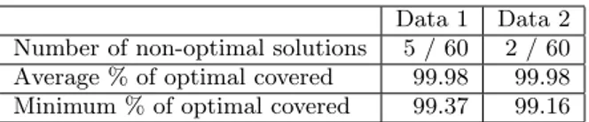
Table 1: Results from comparing the greedy and optimal maximum coverage algorithms.
Data 1 Data 2
Number of non-optimal solutions 5 / 60 2 / 60
Average % of optimal covered 99.98 99.98
Minimum % of optimal covered 99.37 99.16
In this experiment, we have 60 days of sales data from the book store and the hardware store (this is a different set of sales data from the one used in Section 4) that we call Data 1 and Data 2 respectively. We make runs through the data sets and compare the results from greedy with optimal solutions using a session based ageing window with a size of 5 000 sessions. For each day in the data set we calculate an optimal M-list and an approximate M-list and compare the number of customers covered. Table 1 shows the number of times the greedy algorithm found a non-optimal solution and the total number of days in the first row, an average of the number of customers covered by the greedy solution compared to the number of customers covered by the opti-mal solution in percent in the second row, and how close to the optimum the greedy algorithm is, in the worst case in percent in the third row.
As we can see in Table 1, the greedy algorithm finds an optimal solution most of the times for our data. On the few cases where it does not, it is still almost optimal. Our experiments show that we can use the greedy solution as an accurate and practical solution to the maximum coverage problem.
4.
RESULTS
In this section we show results from the evaluation described in Section 2.5. All lists contain k = 10 products and they are all updated once per day (at midnight).
4.1
Data A — The Book Store
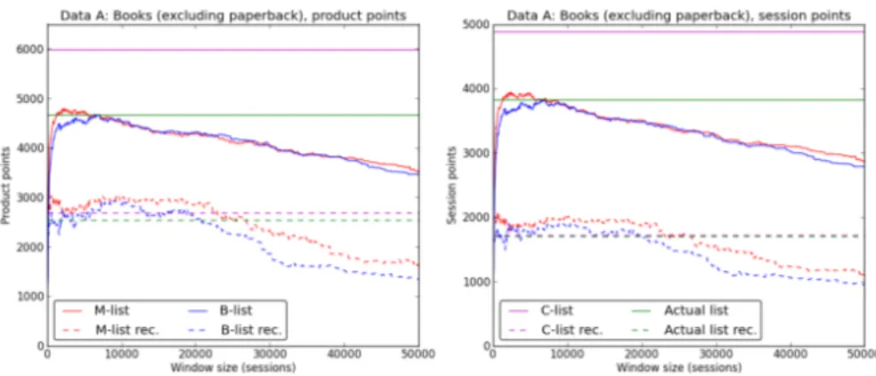
Figure 1 presents the experimental results from our tests on the book store. In both plots, we display in order from the top, the C-list in magenta, the M-list in red, the B-list in blue and the A-list in green. The dashed curves below are points given for recommendations associated to the list of the same color. For each list we count the total number of product (left) and session (right) points accumulated during
Figure 1: Plots over product points (left plot) and session points (right plot) for Data A for M-list (red) and B-list (blue) for different window sizes and lines for C-list (magenta) and the A-list (green). Dashed lines are points for the recom-mendations.
Figure 2: Plots over product points (left plot) and session points (right plot) for Data B for M-list (red) and B-list (blue) for different window sizes. Dashed lines are points for the recommendations.
Figure 3: Plots over total product points (including points for recommendations) for M-list (red) and B-list (blue), for Data A (left plot) and Data B (right plot). Note the different axes.
the 30 day period. Note that the horizontal axis shows the size of the ageing window. In the left plot, the B-list obtains its maximum product points of 4680 points for a window size of 6500. The M-list obtains its maximum of 4702 points for a window size of 1750, i.e., for a significantly shorter window. The A-list counts 4669 product points and the C-list counts 5988 product points. In the right plot, the B-list obtains its maximum session points of 3834 points for a window size of 6500 and the M-list obtains its maximum of 3947 points for a window size of 2300. Counting either the maximum product or session points, the M-list is actually better than the A-list in both cases even without taking PARs into account. The A-list counts 3828 product points and the C-list counts 4885 product points.
In the left plot of Figure 3, we display the sum of prod-uct points for the B-list and its PARs in blue and similarly for the M-list in red. This sum maximizes at 7400 with a window size of 6500 for the accumulated B-list. The ac-cumulated M-list maximizes at 7639 with a window size of 1750. This gives us a ratio between the accumulated maxima of 1.032, hence, a 3% improvement in sales in comparison to the B-list. The accumulated A-list in turn, counts 7214 product points, giving us a ratio of 1.058, hence almost a 6% improvement.
4.2
Data B — The Hardware Store
The results for the hardware store are similar but with even more pronounced differences between the two lists.
In Figure 2, the results for the hardware store are shown. Here we only display the B-list in blue and the M-list in red together with their associated recommendation points as dashed curves. For each list we count the total number of product (left) and session (right) points accumulated during the 30 day period. Again, the horizontal axis shows the size of the ageing window. In the left plot, the B-list obtains its maximum product points of 1820 points for a window size of 1500. The M-list obtains its maximum of 1645 points for a window size of 3100. In the right plot, the B-list obtains its maximum session points of 799 points for a window size of 2450 and the M-list obtains its maximum of 896 points for a window size of 3100.
In the right plot of Figure 3, we again display the sum of product points for the B-list and its PARs in blue and simi-larly for the M-list in red. This sum maximizes at 2432 with a window size of 1400 for the accumulated B-list. The ac-cumulated M-list maximizes at 2629 with a window size of 3100. This gives us a ratio between the accumulated maxima of 1.081, hence, an 8% improvement in sales.
4.3
Effect of PARs
To include the effect of product recommendations in the comparison between the M-list and the B-list we use a linear model where the effect of a list X is calculated as PX+wRX, where PX and RX are the product points for the X-list and its recommendations respectively. The factor w denotes the probability that a customer takes notice of the PARs, the PAR probability. In Section 7 we discuss some ways to design a site to achieve a high w. In Figure 3 we show the results for product points for both data sets with w = 1. In Table 2 we show ratios of M-list points and B-list points for different w.
A fixed window size is used per row, chosen to optimize the list in the “Opt.” column. A ratio larger than 1 means that the M-list is better. For both data sets we establish that the M-list is better than the B-list for all w above 0.58. In other words, the M-list approach is proven better than the B-list if customers take notice of product recommendations at least 58% of the times.
Table 2: Ratios between the M-list and the B-list that take PARs into account.
Data Opt. w 0 0.25 0.5 0.75 1 A B-list 0.990 1.000 1.007 1.013 1.018 A M-list 1.079 1.089 1.097 1.103 1.108 B B-list 0.891 0.943 0.988 1.028 1.062 B M-list 0.914 0.977 1.031 1.078 1.120
4.4
Window Time Span Distributions
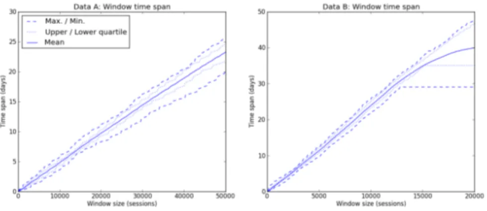
Since the window size is measured in sessions, the time span of the window varies with the session rate. As can be seen in Figure 4, the time span increase is essentially linear with the increase in window size, with slight “waves” due to the cyclic nature of the session rate, with both daily and weekly cycles. The reason for the atypical behavior in the right plot in Figure 4 is that for large window sizes there is not enough data to “fill up” the window before evaluation starts as there is only about a month of “warm up” data.
5.
DIVERSIFICATION
A product list should be both relevant and reflect several aspects of interest. An item in the list, although relevant, might be too similar to a better item in the list and should therefore be replaced by a different item. There exist many methods to achieve such diversification [4, 10, 21, 22]. Our optimization criterion for the M-list tries to diversify users, so we also expect some sort of diversification effect over the products in the M-list in our experiments.
Modifications of classical information retrieval metrics have been used to measure both relevance and diversification [1], but they require predefined manual relevance judgments. Since relevance is covered in Section 4, we now focus on measuring diversification. Most products in our data have one or more associated categories. Typically, products from different categories are not similar. We therefore look at product categories to measure diversification.
As we want to be able to compare products, and each prod-uct may be associated with a set of categories, we apply a distance measure between sets of categories. The most common measure used for sets is the Jaccard distance. The distance J between two sets Ciand Cj, is defined as:
J (Ci, Cj) = 1 −
|Ci∩ Cj| |Ci∪ Cj| .
In our case, Ciand Cjrepresents the set of categories related to product Siand Sjrespectively. With some modifications to handle products with no categories, the measure gives values between 0 and 1, where 0 means that the two prod-ucts have identical categories and 1 means that the prodprod-ucts share no categories.
Figure 4: Plots over window time span for Data A (left plot) and Data B (right plot). Dashed lines are minimum/maximum values, dotted lines are upper and lower quartiles and solid lines are averages. Note the different axes.
For a list of products, L, we define the function D(L) as the average distance between all pairs of sets in L using the Jaccard measure J , or D(L) = P Si∈L P Sj∈(L\{Si})J (Ci, Cj) |L|(|L| − 1) .
This function can be used to get a value from 0 (all products have the same categories) to 1 (all products have unique categories) as a measure of the diversity of a list.
Table 3: Diversification results. Average, standard
deviation and a five-number summary for D-values on lists updated at midnight each day. A session-based window of size 5000 was used.
Data A Data B
M-list B-list M-list B-list
Average 0.862 0.847 0.870 0.728 Standard deviation 0.033 0.065 0.021 0.038 Minimum 0.800 0.644 0.848 0.667 Lower quartile 0.844 0.822 0.848 0.712 Median 0.856 0.856 0.864 0.742 Upper quartile 0.889 0.900 0.894 0.758 Maximum 0.922 0.956 0.909 0.803
Table 3 shows the diversification results between the pre-sented products in the two lists when only the top level categories associated to each product for both data sets are used. For Data A, this gives 26 categories for 41 951 prod-ucts. (6.83% of these are uncategorized, i.e., they have Jac-card distance 1 to all other products.) For Data B we have 16 top level categories and here each of the 4 093 products belongs to at most one category. (1.69% are uncategorized in this set.) The table would change only slightly if we made measurements using the full category trees for the data sets. On average, the M-list achieves a higher diversification value than the B-list for both Data A and Data B. Note, however, that the M-list has lower upper quartile and lower maximum values than the B-list for Data A. Together with the lower standard deviation this indicates that the M-list gives a more consistent diversification although not necessarily higher in all cases. For Data B, the B-list has relatively low diversifica-tion and therefore there is more room for improvement. The
results for the M-list are diversification values comparable to the M-list results for Data A but with even smaller standard deviation. Also note that the improvement for Data B is so large that the minimum value for the M-list is larger than the maximum value for the B-list.
It is important to note that the improved diversification on the presented products is a side-effect of the maximum cov-erage algorithm. We make no claims on the diversification on sales, although it is a natural assumption that increased diversification in recommendations will also lead to increased diversification in sales [8].
6.
ANALYSIS
Our experiment show that our maximum coverage method is consistently better than the best-seller by 3% for the Data A and 8% for the Data B; see Figure 3.
It can be argued that our experiments are not truly valid since we rely on recorded data to express potential sales on future data. In fact, the A-list presented on the book site may not be the same as the B-list computed, hence, the impact that A-list has on sales does not adequately reflect the impact that either the B-list or the M-list would have had on the sales. However, there is no doubt that the B-list approximates the behavior of the A-B-list. Hence, if the M-list can beat the B-list already in our experiments then it makes a strong case in favor of the new algorithm. This is due to so called false negatives. These are cases when customers would have bought a product if we showed it to them. Since we cannot discern the positive effect of showing such products by looking only at historical data, we fail to give the new algorithm points it would have scored if run on a live experiment.
7.
FROM THEORY TO PRACTICE
How can we use the insights given from our research on actual e-commerce sites? If we want to optimize for profit, we need to design the site in accordance with our findings. Below we go through the steps necessary to accomplish this. Our main conclusion is that e-commerce sites place product recommendations too deep into the site structure (typically
on product pages) to be efficiently used while browsing the site. The probability that a customer follows a recommenda-tion link located on a product page, while browsing the site is far too small. Instead, we suggest that recommendation links are added to product list items, for example as a badge on the product picture with the text “More like this”. The “More like this” toggle shows a set of product recommenda-tions as the user hovers over a product. This is especially efficient on landing pages such as the start page, since we know that such pages contribute to a large part of the sales. It is as if we have increased the number of products visible on the page and we rely on what we call natural navigation to make sure that all hidden products are readily obtainable through intuitive product associations, PARs.
Natural navigation is navigation through the site following
recommendations. Since PARs normally are of the type
“Those who bought this also bought. . . ” there is an in-creased risk of cyclic navigation patterns if they are used together with the B-list, especially if the product list con-tains products related to each other. Once a customer has entered such a cycle, natural navigation cannot exit from it. To avoid such cycles and to make sure that the number of products spanned by each page is as large as possible, the e-commerce ranking system should include the maximum coverage algorithm.
Our experiments have been restricted to recommendations from the complete product catalogue. As a customer browses a site, he restricts the product selection, but the recommen-dation problem remains the same. The maximum coverage algorithm can thus be applied to any product list on the site.
8.
CONCLUSIONS
We observe that to optimize sales on an e-commerce site, the first step is to optimize the number of converting customers, and then do up-sales on them. This suggests that all mar-keting lists should be optimized with this in mind. However, today’s sites normally sort their product listings on popu-larity, which as we have shown is not optimal. We demon-strate a new approach based on the maximum coverage al-gorithm that better optimizes sales, with an improvement of 3–8%. A secondary effect that our algorithm exhibits on the tested data is measurably increased diversification in presented products.
An extension of maximum coverage is to use it to optimize entire pages. This extension would also make optimizations between different lists displayed on a page, making the lists aware of each other. One benefit of this optimization method is to avoid showing duplicate information on multiple lists.
9.
REFERENCES
[1] R. Agrawal, S. Gollapudi, A. Halverson, and S. Ieong. Diversifying search results. In Proceedings of
WSDM’09, pages 5–14, 2009.
[2] N. Alon, B. Awerbuch, and Y. Azar. The online set cover problem. In Proceedings of STOC’03, pages 100–105, 2003.
[3] N. Buchbinder and J. Naor. The design of competitive online algorithms via a primal-dual approach.
Foundations and Trends in Theoretical Computer Science, 3(2–3):93–263, 2009.
[4] H. Chen and D.R. Karger. Less is more: probabilistic models for retrieving fewer relevant documents. In Proceedings of ACM SIGIR’06, pages 429–436, 2006. [5] V. Chvatal. A greedy heuristic for the set-covering
problem. Mathematics of Operations Research, 4(3):233–235, 1979.
[6] T.H Cormen, C. Stein, R.L. Rivest, and C.E. Leiserson. Introduction to algorithms. McGraw-Hill Higher Education, 2nd edition, 2001.
[7] U. Feige. A threshold of ln n for approximating set cover. Journal of the ACM, 45(4):634–652, 1998. [8] D.M. Fleder, K. Hosanagar and A. Buja.
Recommender systems and their effects on consumers: the fragmentation debate. In Proceedings of EC’10, pages 229–230, 2010.
[9] M.R. Garey and D.S. Johnson. Computers and intractability: a guide to the theory of
NP-completeness. W.H. Freeman and Company, 1979. [10] S. Gollapudi and A. Sharma. An axiomatic approach
for result diversification. In Proceedings of WWW’09, pages 381–390, 2009.
[11] D.S. Hochbaum. Approximation algorithms for the weighted set covering and node cover problems. SIAM Journal of Computing, 11(3):555–556, 1982.
[12] D.S. Hochbaum, editor. Approximation algorithms for NP-hard problems. PWS Publishing Company, 1997. [13] D.S. Johnson. Approximation algorithms for
combinatorial problems. Journal of Computer and System Sciences, 9:256–278, 1974.
[14] R.M. Karp. Reducibility among combinatorial problems. In R.E. Miller and J.W. Thatcher, editors, Complexity of Computer Computations, pages 85–103. Plenum Press, 1972.
[15] J. Langford, A. Strehl, and J. Wortman. Exploration scavenging. In Proceedings of ICML’08, pages 528–535, 2008.
[16] A. Lipkus. A proof of the triangle inequality for the Tanimoto distance. Journal of Mathematical Chemistry, 26(1):263–265, oct 1999.
[17] T. Malmer. Time-dependent predictions of user purchases on e-commerce sites. Master’s thesis, Lund University, 2011.
[18] B. Saha and L. Getoor. On maximum coverage in the streaming model & application to multitopic
blog-watch. In Proceedings of SIAM SDM’09, pages 697–708, 2009.
[19] S.K. Stein. Two combinatorial covering theorems. Journal of Combinatorial Theory, Series A, 16(3):391–397, 1974.
[20] V.V. Vazirani. Approximation algorithms. Springer-Verlag, 2001.
[21] M.R. Vieira, H.L. Razente, M.C. Barioni,
M. Hadjieleftheriou, D. Srivastava, C. Traina, and V.J. Tsotras. On query result diversification. In Proceedings of ICDE’11, pages 1163–1174, 2011. [22] C. Yu, L. Lakshmanan, and S. Amer-Yahia. It takes
variety to make a world: Diversification in
recommender systems. In Proceedings of EDBT’09, pages 368–378, 2009.