2005:55 Application of Master Curve Methodology for Structural Integrity Assessments of Nuclear Components

SKI Report 2005:55

Research

Application of Master Curve Methodology

for Structural Integrity Assessments of

Nuclear Components

Iradj Sattari-Far

Kim Wallin

October 2005

SKI perspective

Background

Ferritic steels are widely used in different kinds of constructions. One problem with this material is that in the transition region the fracture toughness decreases drastically as the temperature drops. In this region the final failure is often occurred by cleavage preceded by some ductile crack growth. A procedure for mechanical testing and statistical analysis of fracture toughness of this type of materials is describing in the ASTM E 1921-03 standard. The above mentioned standard is accounting for temperature dependence of fracture

toughness through an approach developed by Kim Wallin, widely known as Master Curve method. Wallin has observed that a wide range of this type of material has a characteristic shape of the fracture toughness-temperature curve, and the only difference between different steels is the absolute position of the curve with respect to temperature. The temperature dependence of fracture toughness can be determined by performing a certain amount of fracture toughness tests at a given temperature.

Results of the application of Master Curve method for evaluation of fracture toughness in the transition region have shown that this method relaxes some of the over-conservatism which has been observed in using the ASME method, generally known as ASME KIC reference curve.

At this time, several countries have adopted or are in the process of adopting the Master Curve method into their brittle fracture safety assessment procedures (Finland, Germany, USA etc.). In Sweden, the ASME KIC reference curve is still used as the only approved method in safety evaluations.

Objective

The objective was to perform an in-depth investigation of the Master Curve methodology and also based on this method develop a procedure for fracture assessments of nuclear

components. The results of this study will be used for the SKI´s position on whether the Master curve methodology will be adopted into our brittle fracture assessment procedures.

Results

The project has sufficiently illustrated the capabilities of the Master Curve methodology for fracture assessments of nuclear components. Within the scope of this work, the theoretical background of the methodology and its validation on small and large specimens has been studied and presented to a sufficiently large extent, as well as the correlations between the charpy-V data and the Master Curve T0 reference temperature in the evaluation of fracture toughness. The work gives a comprehensive report of the background theory and the different applications of the Master Curve methodology.

The main results of the work have shown that the cleavage fracture toughness is characterized by a large amount of statistical scatter in the transition region, it is specimen size dependent and it should be treated statistically rather than deterministically. The Master Curve

Furthermore, the Master Curve methodology provides a more precise prediction of the

fracture toughness of embrittled materials in comparison with the ASME KIC reference curve, which often gives over-conservative results.

The suggested procedure in this study, concerning the application of the Master Curve method in fracture assessments of ferritic steels in the transition region and the low shelf regions, is valid for the temperatures range T0-50≤T≤T0+50 0C. If only approximate information is required, the Master Curve may well be extrapolated outside this temperature range. The suggested procedure has also been illustrated for some examples.

The primary objective to provide sufficient information about the Master Curve methodology is now considered to be fulfilled. The SKI assessment is that for the time being there is no immediate need for further studies.

Project Information

SKI´s project leader: Konstantinos Xanthopoulos. Project Number: 14.42-031047/23131.

Project Organisation: Det Norske Veritas AB Consulting (DNV) has been managing the project and has also worked as the principal investigator, with Iradj Sattari-Far as project leader. Peter Dillström at DNV and Kim Wallin at VTT in Finland have assisted this work.

SKI Report 2005:55

Research

Application of Master Curve Methodology

for Structural Integrity Assessments of

Nuclear Components

Iradj Sattari-Far¹

Kim Wallin²

¹Det Norske Veritas

Box 30234

SE-104 25 Stockholm

Sweden

²VTT

P.O. Box 1000

FI-02044 VTT

Finland

October 2005

This report concerns a study which has been conducted for the Swedish Nuclear Power Inspectorate (SKI). The conclusions and viewpoints presented in the report are those of the author/authors and do not

Table of Content

Page

ACKNOWLEDGEMENT... 3

1. INTRODUCTION ... 5

2. BACKGROUND... 7

2.1. Brittle fracture... 8

2.2. LEFM KIC versus EPFM KJC... 12

3. THEORETICAL BASIS OF THE MASTER CURVE METHOD ... 15

3.1. Mechanism of cleavage fracture ... 15

3.2. Probability of cleavage initiation... 20

3.3. Conditional cleavage propagation ... 24

4. DETERMINATION OF MASTER CURVES ... 35

4.1. Comparison of Master Curve KJC and ASME KIc... 39

5. MASTER CURVE ANALYSIS OF SMALL SPECIMENS... 41

5.1. Master Curve analysis of miniature specimens ... 42

5.2. Test results of other small specimens ... 52

5.3. Comparison of CT- and 3PB-specimens ... 61

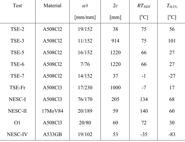
6. MASTER CURVE ANALYSIS OF LARGE SCALE EXPERIMENTS... 65

6.1. Experiment TSE-2 at ORNL... 66

6.2. Experiment TSE-3 at ORNL... 69

6.3. Experiments TSE-5 and TSE-6 at ORNL... 70

6.4. Experiment TSE-7 at ORNL... 73

6.5. Experiment TSE-FR at Framatome ... 75

6.6. Experiment NESC-I at AEA... 78

6.7. Experiment NESC-II at MPA ... 79

6.8. Experiment O1 at KTH... 82

6.9. Experiment NESC-IV at ORNL ... 84

6.10. Experiments PTSE-1 and PTSE-2 at ORNL ... 88

7. CONSTRAINT EFFECTS ... 90

7.1. Stress field around a crack tip... 91

7.2. Constraint parameters ... 94

7.3. Constraint considerations in the Master Curve Methodology ... 100

7.3.1. Constraint considerations of small specimens ... 100

7.4. Constraint correction for surface cracks ... 116

8. CORRELATION BETWEEN CHARPY IMPACT CVN AND T0 ... 119

8.1. Charpy-V – T0 correlations for nuclear grade pressure vessel steels ... 120

8.2. Relation between T28J and T41J... 125

8.3. Analysis of complete CVN transition curves ... 125

8.4. Analysis of incomplete CVN transition curves ... 133

8.5. CVN-To relationships ... 137

8.6. Significance of ASME Code Cases N-629 and N-631 ... 137

9. APPLICATION OF THE MC METHOD IN OTHER COUNTRIES... 145

10. ASSESSMENT PROCEDURE BASED ON THE MC METHOD... 147

10.1. Simplified assessment procedure... 147

10.2. Advanced assessment procedure ... 150

11. CONCLUSIONS AND RECOMMENDATIONS... 154

REFERENCES ... 156

ACKNOWLEDGEMENT

This research project is sponsored by the Swedish Nuclear Power Inspection (SKI) under contract: SKI-14.42-031047/23131. This support is greatly appreciated. The authors are delighted to thank Björn Brickstad and Kostas Xanthopoulos (SKI) for their support and encouragement over the course of this project.

1. INTRODUCTION

Integrity assessment of structures containing planar flaws (real or postulated) requires the use of fracture mechanics. Fracture mechanics compares, in principle, two different crack growth parameters: the driving force and the material resistance. The driving force is a combination of the flaw size (geometry) and the loading conditions, whereas the material resistance describes the materials capability to resist a crack from propagating. Up to date, there exist several different testing standards (and non-standardised procedures) by which it is possible to determine some parameters describing the materials fracture resistance (ASTM E 399, ASTM E 1820, BS 7448, ESIS P2 etc.). Unfortunately, this has led to a myriad of different parameter definitions and their proper use in fracture assessment may be unclear.

Historically, fracture mechanics evolved from a continuum mechanics understanding of the fracture problem. It was assumed that there existed a single fracture toughness value controlling the materials fracture. If the driving force was less than this fracture toughness, the crack would not propagate and if it exceeded the fracture toughness the crack would propagate. Thus, crack initiation and growth were assumed to occur at a constant driving force value. The only thing assumed to affect this critical value was the constraint (crack-tip stress triaxiality) of the specimen (or structure). Since, at that time, there were no means to quantitatively assess the effect of constraint on the fracture toughness, the fracture toughness had to be determined with a specimen showing as high a constraint as possible. This leads to the use of, deeply cracked, bend specimens for the fracture toughness determination. It was assumed that the stress state assumption of the continuum mechanics analysis were valid for fracture toughness as well, regardless of fracture micro-mechanism. This statement has later been proven to be wrong. Different fracture micro-mechanisms exhibit different physical features that affect the validity of a specific fracture toughness parameter to describe that fracture micro-mechanism.

The ASTM E 1921-03 standard [2003] describes a procedure for the mechanical testing and statistical analysis of fracture toughness of ferritic steels in the transition region. This ASTM standard accounts for temperature dependence of fracture toughness through a Master Curve approach developed by Wallin [1991]. Wallin observed that a wide range of ferritic steels have a characteristic fracture toughness-temperature curve, and the only difference between

different steels was the absolute position of the curve with respect to temperature. The temperature dependence of the fracture toughness can be determined by performing a certain amount of fracture toughness test at a given temperature. Using the Master curve for evaluation of the fracture toughness in the transition region releases the over-conservatism that has been observed in using the ASME KIC curve. The application of the Master Curve

methodology in prediction of the fracture events in nuclear components has shown promising results, see for instance Bass et al [2000], Sattari-Far [2000 and 2004] and Wallin [2004c]. The primary objective of this report is to establish a straight forward procedure in application of the Master Curve methodology in fracture assessments of the nuclear components. In performing this task, the background of the methodology and its validation are studied.

Chapters 2 and 3 give background and theoretical aspects of the methodology, emphasizing the probabilistic handling of fracture toughness data. Chapter 4 briefly describes the procedure for performing fracture toughness testing and determination of the Master Curves according to the ASTM E1921 standard. Chapter 5 gives results of application of the Master Curve methodology in determination of validated fracture toughness from miniature sized test specimens. The validation of the methodology in predictions of fracture events in large scale experiments are investigated in Chapter 6. The capability of the methodology in considering the constraint effects are examined in Chapter 7. As in the cases of existing nuclear power plants, fracture toughness data are often not available and the available material information is often limited to Charpy-V test results, correlations between the impact energy and the Master Curve fracture toughness are therefore given in Chapter 8. Chapter 9 gives information on application of this methodology in different countries.

Based on the results presented in Chapters 1-9, a procedure on how to apply this methodology is developed and presented in Chapter 10. The use of this procedure is demonstrated in Appendix of this report, using some realistic examples. Finally, Chapter 11 concludes this report and gives recommendations on how to use this methodology.

2. BACKGROUND

Fracture mechanics, based on a continuum mechanics, gives means in understanding of fracture behaviour in cracked bodies. It is commonly assumed that there exists a single fracture toughness value controlling the materials fracture. If the crack driving force in the body is less than this value, the crack will not propagate and if it exceeds this value the crack will propagate.

The concept of linear elastic fracture mechanics (LEFM) that was derived prior to 1960 is applicable only to structures whose global behaviour are linear. In application of LEFM, the crack-tip field in a cracked body is described by the stress intensity factor, K, provided that certain conditions are satisfied. LEFM is valid for the cases in which the nonlinear material behaviour is confined to a small region surrounding the crack tip. In other cases, it is virtually impossible to characterize the fracture behaviour with LEFM, and an alternative fracture mechanics model is required. Since 1960, fracture mechanics theories have been developed to account for various types of non-linear material behaviour and loading condition. Elastic-plastic fracture mechanics (EPFM) approaches based on elastic-Elastic-plastic parameters, the J-integral or the crack-tip opening displacement (CTOD), extend the limitations of LEFM. Both parameters describe crack-tip conditions in elastic-plastic materials, and each can be used as a fracture criterion. There are, however, limits to the applicability of J or CTOD, but these limits are much less restrictive than the validity requirements of LEFM.

The crack-tip field and the fracture toughness are only geometry independent within a limited range of loading and geometric conditions, which ensures similar crack-tip stress triaxiality (constraint). The size and geometry requirements restrict the application of different fracture mechanics disciplines. Under small scale yielding (SSY) conditions, a single parameter (e.g. K, J or CTOD) characterizes crack-tip conditions and thus can be used as a geometry-independent fracture criterion. At increasing loads in finite cracked bodies, the initially SSY field gradually diminishes as the plastic zone senses nearby traction free boundaries. Consequently, the single-parameter fracture mechanics disciplines break down, and the fracture toughness depends on the size and geometry and type of loading of the fractured body. A number of approaches have been proposed to extend fracture mechanics applications beyond the limits of the single-parameter assumptions. Most of these new approaches involve

the introduction of a second parameter to characterize the crack-tip conditions, so called two-parameter fracture mechanics approaches.

2.1. Brittle fracture

Two models claiming to predict the temperature dependence of cleavage fracture toughness are the RKR-model (Ritchie, Knott & Rice) and the Beremin model (known as the local approach). Both models essentially assume a constant cleavage fracture stress (σc, σu) and end up with similar results for the temperature dependence. It may be somewhat misleading to talk about temperature dependence, since the models actually predict an inverse dependence between fracture toughness and yield strength:

KIC ∼ σy-c (2-1)

Both models yield for a moderately strain hardening material (n = 10) having the “standard” Weibull slope (m = 22) c = 4.5.

The models were originally verified for materials with the ductile to brittle transition occurring at low temperatures, where the change in yield strength with temperature was considerable. However, for more brittle materials, where the ductile to brittle transition occurs above room temperature, the models are unable to predict the temperature dependence correctly [Merkle, Wallin and McCabe, 1998]. Wallin [2004] studied fracture toughness data of A533B Cl.1 in both unirradiated and irradiated conditions. He came to the following postulate:

• The temperature dependence of cleavage fracture toughness is mainly controlled by the thermal part of the materials yield strength, whereas the location on the temperature scale is more controlled by the athermal part of the yield strength.

Based on this postulate, a unified description of the fracture toughness temperature dependence for ferritic steels may be possible.

Even though materials failing by cleavage fracture were not part of the development of the KIC standards, it soon became applied to testing of nuclear pressure vessel steels. Actually,

suited for brittle fracture. This is a misconception, coming from the erroneous interpretation of plane-strain coming from the Irwin investigation. Also in the case of brittle fracture, the original continuum mechanics based interpretation was assumed, i.e. that valid KIC results are

lower bound specimen size insensitive material values showing only little scatter. Based on the present understanding of the physics of the cleavage fracture micro-mechanism, this assumption is known to be incorrect, [Wallin, 2004].

Based on an interpretation of the physics, the Master Curve method was developed at VTT. The method adjusts for size effects in brittle fracture toughness. Physically, the fracture toughness in temperature space can be divided into three regions, brittle fracture region, transition region and upper shelf. The brittle fracture region is further divided into two separate regions, depending on the way specimen size affects the fracture toughness. In the lower shelf region, size effects are negligible, but at higher toughness values, the brittle fracture toughness will be affected by a statistical size effect. The transition region is defined as the temperature region, where cleavage fracture occurs after some amount of ductile tearing. This region will be specimen size dependent due to the statistical size effect. Finally, the upper shelf is defined as the temperature region where the fracture mechanism is fully ductile. Also the temperature for the onset of upper shelf is specimen size dependent due to the statistical size effect. Besides, statistical size effects, the fracture toughness can be affected by specimen constraint. The basic Master Curve has been standardised by ASTM in ASTM E 1921-03, [ASTM, 2003].

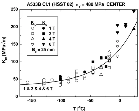
The statistical size effect, due to the weakest link nature of cleavage fracture initiation, is active also for valid KIC results, provided they are above the lower shelf. A good example of

this is given by the HSST 02 plate data used originally to develop the ASME KIC reference

curve shown in Fig. 2.1, [Marston, 1978]. The data, originally known as the "million dollar curve", constituted the first large fracture toughness data set generated for a single material. Normally, only the valid KIC results are reported, but for clarity, here also the invalid results

are included. It is evident that there is a difference between the smaller 1T & 2T specimens and the larger 4T & 6T specimens. This size effect, shown in Fig. 2.2, is fully in line with the theoretical statistical size effect as used by the Master Curve methodology.

-150 -100 -50 0 0

50 100 150

A533B Cl.1 (HSST 02) σ_Y = 480 MPa CENTER

4 & 6 T 1 & 2 T K IC [M Pa √m] T [oC] K_IC K_Q 1 T 2 T 4 T 6 T

Fig. 2.1. Valid brittle fracture KIC data for the HSST 02 plate indicating decreasing fracture

toughness with increasing specimen size, [Marston, 1978].

-150 -100 -50 0 0 50 100 150 200 250

A533B Cl.1 (HSST 02) σ_Y = 480 MPa CENTER

1 & 2 & 4 & 6 T

K_IC K_Q 1 T 2 T 4 T 6 T B₀ = 25 mm T [oC] K IC [M P a √m]

Fig. 2.2: Size effect in valid brittle fracture KIC data for the HSST 02 plate is correctly

Another example showing the decrease in KIC with increasing specimen size has been

presented by MPA, shown in Fig. 2.3, [Issler, 1979]. Even though the data are limited in number, it clearly indicates decreasing fracture toughness with increasing specimen size, for all valid KIC values. Also in this case, the size effect is in line with the theoretical prediction

of the Master Curve. Numerous similar data sets can easily be found in the open literature.

0 20 40 60 80 100 120 140 0 20 40 60 80 100 120 140 50 % 5 % 95 % ASTM E399 limit

K IC [M P a √ m] B [mm] MPA CT DATA 20 MnMoNi 5 5 T_NDT = -20oC T = -100oC

Fig. 2.3: MPA brittle fracture KIC data, for KS13, showing size effect in accordance with the

Master Curve, [Issler, 1979].

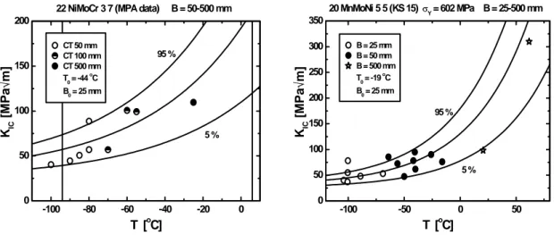
Within the same nuclear safety research programme, MPA has also tested three "gigantic" CT specimens with 500 mm thickness, [Kussmaul et al, 1986]. One specimen corresponded to material KS05 and two to KS15. The results, together with smaller specimen valid KIC results

are presented in Fig. 2.4. A clear size effect can be seen. The very large specimens provide clearly lower fracture toughness values than predicted based on the smaller specimen behaviour.

If the data is analysed and size adjusted with the Master Curve, the different specimen sizes are in much better agreement, shown in Fig. 2.5. It should be pointed out that the specimens in question have been produced from different forgings, and slightly different NDT values have

been reported for the small and large specimen materials, [Kussmaul et al, 1986]. Overall, the evidence is however clear. KIC in the case of brittle fracture is not a deterministic limiting

lower bound value. It has the same kind of size effect as KJC values corresponding to cleavage

fracture and they need to be analysed by the Master Curve.

-100 -80 -60 -40 -20 0 0

50 100 150

22 NiMoCr 3 7 (MPA data) B = 50-500 mm

CT 50 mm CT 100 mm CT 500 mm KIC [MPa √ m] T [oC] -100 -50 0 50 0 50 100 150 200 20 MnMoNi 5 5 (KS 15) σ_Y = 602 MPa B = 25-500 mm B = 25 mm B = 50 mm B = 500 mm KIC [MPa √ m] T [oC]

Fig. 2.4: MPA brittle fracture KIC data, for KS05 and KS15, showing size effect for valid KIC

values, [Kussmaul et al, 1986].

-100 -80 -60 -40 -20 0 0 50 100 150 200 5 % 95 %

22 NiMoCr 3 7 (MPA data) B = 50-500 mm

CT 50 mm CT 100 mm CT 500 mm T₀ = -44 o C B0 = 25 mm KIC [M Pa √ m] T [oC] -100 -50 0 50 0 50 100 150 200 250 300 350 5 % 95 % 20 MnMoNi 5 5 (KS 15) σ_Y = 602 MPa B = 25-500 mm B = 25 mm B = 50 mm B = 500 mm T0 = -19 o C B₀ = 25 mm KIC [MP a √ m] T [oC]

Fig. 2.5: MPA brittle fracture KIC data, for KS05 and KS15, showing size effect to be in

accordance with the Master Curve.

2.2. LEFM K

IC

versus EPFM K

JC

The common misconception, originating from the erroneous interpretation of conditions required for plane-strain fracture toughness, is to assume that only valid KIC results

to be a criteria for plane-strain. In reality, the requirements are intended to ensure the applicability of linear-elastic fracture mechanics, so that the fracture toughness can simply be estimated from load information. The requirements have nothing to do with the limiting conditions for plane-strain stress state in front of the crack. Modern finite element analyses have shown that the specimen thickness can be reduced by more than a factor of 10, from the ASTM E399 criterion, without loss of the plane-strain stress state. The main difference between KIC and KJC is that, KJC has to be estimated via the elastic-plastic parameter J, which

requires the measurement of both load and load-point displacement. As long as the KJC values

fulfil the size requirements given in ASTM E1921, they are of equal significance as valid KIC

values for cleavage fracture. In both cases, the fracture toughness is affected by the statistical size effect. This means that both KIC and KJC values, in the case of cleavage fracture, have to

be analysed using the Master Curve method.

Fig. 2.6 presents data from McCabe [1993], showing the effect of specimen thickness on the median fracture toughness. The error bars indicate the 90 % confidence bounds of the median estimate. The smaller specimens correspond to elastic-plastic KJC values whereas the 100 mm

thick specimens yield valid linear-elastic KIC values. Regardless of parameter type, all

specimens follow the same size dependence as predicted by the Master Curve. Thus, the size effect is identical to the one seen for valid KIC results, shown e.g. in Fig. 2.3. This shows that

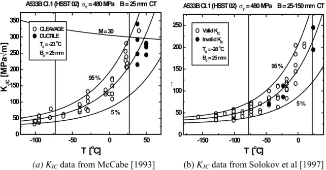
the specimens are not affected by changes in the stress state, only the statistical size effect. Also the HSST 02 plate shows the similarity between KIC and KJC. Fig. 2.7a shows the

original HSST 02 KIC data analysed by the ASTM E1921 Master Curve method. Fig. 2.7b

shows elastic plastic results for the same plate, tested by EPRI and ORNL [Solokov et al, 1997], also analysed by the ASTM E1921 Master Curve method. The KIC data yield a T0

estimate of -28ºC and the KJC yield a T0 estimate of -23ºC. The difference between the two

estimates is only 5ºC. This is very little, since it includes both the statistical uncertainty connected to T0 estimation, as well as the effect of possible material in-homogeneity.

Above only a couple examples of the similarity between KIC and KJC have been given. In the

literature it would be quite easy to find more examples showing the same similarity. However, in order to avoid repetition and since the HSST 02 KIC data forms the basis for the ASME KIC

constituted by HSST 02 provides the best demonstration of the similarity between KIC and KJC. 0 20 40 60 80 100 0 50 100 150 200 95 % 5 % HSST Plate 13A K_25mm = 109 MPa√m K median [MPa √ m] B [mm] Valid K IC E399 limit K_JC Master Curve

Fig. 2.6: Effect of specimen thickness on KJC and KIC fracture toughness explained by the

statistical size effect, [McCabe, 1993].

-100 -50 0 50 0 50 100 150 200 250 300 350 M = 30 5 % 95 % A533B Cl.1 (HSST 02) σ_Y = 480 MPa B = 25 mm CT CLEAVAGE DUCTILE T₀ = -23 oC B 0 = 25 mm KJC [M Pa √ m] T [oC] -150 -100 -50 0 0 50 100 150 200 250 5 % 95 % A533B Cl.1 (HSST 02) σ_Y = 480 MPa B = 25-150 mm CT Valid K IC Invalid K_IC T₀ = -28 oC B₀ = 25 mm IC T [oC]

(a) KIC data from McCabe [1993] (b) KJC data from Solokov et al [1997]

Fig. 2.7: Application of the ASTM E1921 Master Curve analysis to KIC and KJC results of the HSST 02 tests.

3. THEORETICAL BASIS OF THE MASTER CURVE METHOD

The micromechanism of cleavage fracture exhibits a strong sensitivity to the stress field at the crack tip. Moreover, the highly localized phenomenon of cleavage fracture also demonstrates high sensitivity to the random inhomogeneities in the material along the crack front. Consequently, cleavage fracture toughness values which meet the specified size requirements nevertheless display large amount of statistical scatter, especially for temperatures corresponding to the transition region. Because of this substantial scatter, cleavage toughness data should be treated statistically rather than deterministically. It means that a given steel does not have a single value of toughness at a particular temperature in the transition region; rather, the material has a toughness distribution. Testing of numerous specimens to obtain a statistical distribution of the fracture toughness can be expensive and time-consuming. In addition, there has been an interest to utilize small fracture specimens, e.g. of Charpy size, to obtain fracture toughness data when severe limitations exist on material availability, for instance when considering irradiation embrittlement for ferritic materials. To reduce these problems, a methodology has been developed that greatly simplifies the process of determination of fracture toughness in the transition region. The ASTM E 1921-03 standard [2003] describes the procedure for the mechanical testing and statistical data analysis of ferritic steels in the transition region. This ASTM standard accounts for temperature dependence of toughness through a Fracture Toughness Master Curve approach developed by Wallin [1991]. Wallin observed that a wide range of ferritic steels have a characteristic fracture toughness-temperature curve, and the only difference between different steels was the absolute position of the curve with respect to temperature. The temperature dependence of the fracture toughness can be determined by performing a certain amount of fracture toughness tests at a given temperature. A brief description of the theoretical basis of the Master Curve methodology is given below based on NUREG/CR-5504 [Merkle, Wallin and McCabe, 1998].

3.1. Mechanism of cleavage fracture

The different possible mechanisms of cleavage fracture initiation are qualitatively rather well known. Primarily the initiation is a critical stress controlled process, where stresses and strains acting on the material produce a local failure, which develops into a dynamically propagating

cleavage crack. The local “initiators” may be precipitates, inclusions or grain boundaries, acting alone or in combination. An example of a typical cleavage fracture initiation process is presented schematically in Fig. 3.1. The critical steps for cleavage fracture are:

(I) Initiation of a microcrack e.g. fracturing of a second phase particle or grain boundary.

(II) Propagation of this microcrack into the surrounding grains.

(III) Further propagation of the propagating microcrack into other adjacent grains.

σ σ σ σ σ σ

Local stress produces a dislocation pile-up which impinges on a grain boundary carbide.

Cracking of the carbide introduces a microcrack which propagates into the matrix.

Advancing microcrack encounters the first large angle boundary.

KW952D

Fig. 3.1: An example of a cleavage fracture initiation process.

Depending on loading geometry, temperature, loading rate and material, different steps are more likely to be most critical. For structural steels at lower shelf temperatures and ceramics, in the case of cracks where the stress distribution is very steep, steps II and III are more difficult than initiation and they tend to control the fracture toughness. At higher temperatures, where the steepness of the stress distribution is smaller, propagation becomes easier in relation to initiation and step I becomes more and more dominant for the fracture process. The temperature region where step I dominates is usually referred to as the transition region. On the fracture surface of a specimen with a fatigue crack this is usually seen as a difference in the number of initiation sites

initiation sites are visible, whereas at higher temperatures, corresponding to the transition region, only one or two initiation sites are seen. In the case of notched or plain specimens, only a few initiation sites are seen even on the lower shelf. This is due to that, for cracks, the peak stresses are very high virtually from the beginning of loading, whereas for notched and plain specimens, the peak stresses increase gradually during loading. Because no materials are fully uniform on a microscale, cleavage fracture initiation is a statistical event, which have implications upon the macroscopic nature of brittle fracture. A statistical model is thus needed to describe the probability of cleavage fracture, [Merkle, Wallin and McCabe, 1998].

TRANSITION

REGION

LOWER

SHELF

Crack pr

opagation

Fig. 3.2: Typical cleavage fracture surfaces for specimens with cracks. Lower shelf conditions produce numerous initiation sites, whereas in the transition region, only one or two initiation sites are visible.

The basis of a general statistical model is presented in Fig. 3.3. It is assumed that the material in front of the crack contains a distribution of possible cleavage fracture initiation sites i.e. cleavage initiators. The cumulative probability distribution for a single initiator being critical can be expressed as Pr{

I} and

it is a complex function of the initiator size distribution, stress, strain, grain size, temperature, stress and strain rate etc. The shape and origin of the initiator distribution is not important in the case of a "sharp" crack. The only necessary assumption is that no global interaction between initiators exists. This means that interactions on a local scale are permitted. Thus a cluster of cleavage initiations may be required for macroscopic initiation. As long as the cluster is local in nature, it can be interpreted as being a single initiator. All the above factors can

be implemented into the initiator distribution and they are not significant as long as no attempt is made to determine the shape and specific nature of the distribution.

KW962.dsf

σ = stress

V = volume

Pr{I}, N

_σ

Cleavage initiator

distribution

{

Fig. 3.3: Basis of the general statistical model.

If a particle (or grain boundary) fails, but the broken particle is not capable of initiating cleavage fracture in the matrix, the particle sized microcrack will blunt and a void will form. Such a void is not considered able to initiate cleavage fracture. Thus, the cleavage fracture initiator distribution is affected by the void formation, leading to a conditional probability for cleavage initiation (Pr{I/O}).The condition being that the cleavage initiator must not have become a void. The cleavage fracture process contains also an other conditional event, i.e. that of propagation. An initiated cleavage crack must be able to propagate through the matrix in order to produce failure. Thus the conditional probability will be that of propagation after initiation (Pr{P/I}).

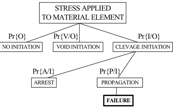
The cleavage fracture initiation process can be expressed in the form of a probability tree as shown in Fig. 3.4.

STRESS APPLIED

TO MATERIAL ELEMENT

NO INITIATION

VOID INITIATION

CLEVAGE INITIATION

PROPAGATION

ARREST

Pr{O}

Pr{V/O}

Pr{I/O}

Pr{A/I}

Pr{P/I}

FAILURE

Fig. 3.4: Probability tree for cleavage fracture. Here, the probabilities of the different events are defined as:

Pr{I} = probability of cleavage initiation Pr{V} = probability of void initiation Pr{O} = probability of “no event”

Pr{I/O} = conditional probability of cleavage initiation (no prior void initiation) Pr{V/O} = conditional probability of void initiation (no prior cleavage initiation) Pr{P/I} = conditional probability of propagation (in the event of cleavage initiation) Pr{A/I} = conditional probability of arrest (in the event of cleavage initiation) The following relations are clear from the probability tree:

Pr{O} + Pr{V/O} + Pr{I/O} = 1 (the sum of probabilities is unity) and

Pr{A/I} + Pr{P/I} = Pr{I/O} (the sum of propagation and arrest equals the

3.2. Probability of cleavage initiation

To simplify derivation it is advisable first to evaluate only the cumulative failure probability of cleavage initiation, leaving propagation to a later stage. Since initiation is controlled by a single local initiator being critical, weakest link statistics is applicable for the process.

Weakest link statistics indicates that at least one initiation is required for failure, which is equal to Pf=1-Sr, where Sr is the survival probability, i.e. the probability of no initiation. The cumulative failure probability of a volume element, with an uniform stress state, can thus be expressed as

{ }

[

_{1 Pr I/O}

]

N 1 f P = − − (3-1)

where N is the number of initiators in the volume element.

The relation between the cleavage initiation probability Pr{I} and the conditional cleavage initiation probability Pr{I/O} is

Pr{I/O} = Pr{I}⋅(1- Pr{V/O}) (3-2) i.e. the probability of cleavage initiation times the probability of not having void initiation. Eq. (3-2) apparently makes a reliable estimation of the overall cleavage initiation probability more difficult. However, it will subsequently be shown that the problem is resolved for a sharp crack in small scale yielding.

Normally the exact number of initiators in a volume element is not known. If, however, the initiators are assumed to be randomly distributed in the material, the number of initiators in a randomly selected volume element will be Poisson distributed. The Poisson distribution has the form:

( )

N! N exp N N N P = ⋅ − (3.3)

where N is the mean number of initiators, related to the mean number of initiators per unit volume ( V N ) by V V N N= ⋅ .

The cumulative cleavage initiation probability, in terms of the mean number of initiators, becomes:

{ }

(

{ }

)

[

]

∑ ∞ = − ⋅ − ⋅ − = 0 N N P N V/O Pr 1 I Pr 1 1 f P (3-4a) or

{ }

(

{ }

)

[

]

{

}

∑ ∞ = − ⋅ − ⋅ − ⋅ − = 0 N N! N e N V/O Pr 1 I Pr 1 N 1 f P (3-4b)

Eq. (3-4b) looks complicated, but it can be simplified by making use of the exponential equation. By definition, the exponential equation can be expressed as

∑ ∞ = = 0 N N! N x x e (3-5) Inserting Eq. (3-5) into Eq. (3-4b) yields the simple form

{ }

(

{ }

)

{

-N Pr I 1 Pr V/O

}

exp 1 f P = − ⋅ ⋅ − (3-6a) or

{ }

(

{ }

)

{

-N_V V Pr I 1 Pr V/O

}

exp 1 f P = − ⋅ ⋅ ⋅ − (3-6b) The previous derivation was for one volume element, but in the case of several (n) independent

volume elements with varying sizes and stresses (Fig. 3.5), the cumulative cleavage initiation probability is obtained by summation

{ }

(

{ }

)

{

}

∑ = − ⋅ ⋅ ⋅ − − = n 1 i V/O i Pr 1 I i Pr i V V N exp 1 f P (3-7)

V

₁

V

₂

V

₃

V

_n

σ

₁

σ

₂

σ

₃

σ

_n

Fig. 3.5: Several independent volume elements.

For a "sharp" crack in small scale yielding the stresses and strains are described by the HRR field. One property of the HRR field is that the stress distribution is self similar and another that the stresses have an angular dependence. The term “small scale yielding” is in this derivation used to describe the loading situation where the self similarity of the stress field remains unaffected by loading. Thus the stress field can be divided into small fan like elements with an angle increment ∆θ (Fig. 3.6). In this case the cumulative cleavage initiation probability is written as:

( )

{ }

{ }

∑ ⎥ ⎥ ⎥ ⎦ ⎤ ⎢ ⎢ ⎢ ⎣ ⎡ ∑ = ⎭⎬ ⎫ ⎩ ⎨ ⎧ _⎟ ⎠ ⎞ ⎜ ⎝ ⎛ − ⋅ ⋅ ∆ ⋅ ⋅ ∆ ⋅ ⋅ − − =

π

θ

θ

θ

θ

2 0 = p x 0 x V/O x, Pr 1 I x, Pr sin x x B V N exp 1 f P (3-8)

where the volume element in the x-direction, described by ∆x must be clearly larger than the initiator size (∆x > ~10 µm). The double summation indicates that the summation is performed over the whole cleavage fracture process zone. The cleavage fracture process zone is essentially restricted to the region of high tensile stresses and plastic strains. For simplicity, the stress distribution is assumed to be uniform over the specimen thickness B (crack front length). Accounting for the thickness dependence of the stress distribution would only lead to the addition of a third summation over the thickness in slices ∆B. As long as the thickness dependence of the stress distribution is independent of KI (small scale yielding), the overall

∆θ

θ

x

∆

x

σ

_yy

f(K

_I

)

Fig. 3.6: Stress distribution in front of a crack showing definitions of ∆θ, θ, x and ∆x. Due to the self similar properties of the sharp crack stress field it is possible to normalize the distance with the stress intensity factor to produce a uniqueness description of the stress distribution: 2 y / I K x U ⎟ ⎠ ⎞ ⎜ ⎝ ⎛ =

σ

(3-9)

When Eq. (3-9) is substituted into Eq. (3-8), the probability of cleavage initiation can be expressed in terms of KI and U, as expressed in Eq. (3-10).

( )

{ }

{ }

⎪ ⎭ ⎪ ⎬ ⎫ ⎪ ⎩ ⎪ ⎨ ⎧ ∑ ⎥ ⎥ ⎥ ⎦ ⎤ ⎢ ⎢ ⎢ ⎣ ⎡ ∑ = ⎭⎬ ⎫ ⎩ ⎨ ⎧ _⎟ ⎠ ⎞ ⎜ ⎝ ⎛ − ⋅ ⋅ ∆ ⋅ ⋅ ∆ ⋅ − ⋅ ⋅ − =

π

θ

θ

θ

θ

σ

2 0 = p U 0 U V/O U, Pr 1 I U, Pr sin U U V N 4 y 4 I K B exp 1 f P (3-10)

The value of the double summation in Eq. (3-10) is always negative and independent of KI.

{

B K4_I constant

}

exp 1 f P = − − ⋅ ⋅ (3-11a) or ⎪ ⎪ ⎭ ⎪⎪ ⎬ ⎫ ⎪ ⎪ ⎩ ⎪⎪ ⎨ ⎧ ⎟ ⎟ ⎟ ⎠ ⎞ ⎜ ⎜ ⎜ ⎝ ⎛ ⋅ − − = 4 0 K I K 0 B B exp 1 f P (3-11b)

where B0 is a freely definable normalisation crack front length and K0 corresponds to a

cumulative initiation probability of 63.2 %.

The remarkable feature of the cumulative cleavage initiation probability distribution is that it is really independent of the local cleavage initiator distribution. The result contains no approximations. The only assumption is that the initiators are independent on a global scale. In other words, it is assumed that the volume elements are independent for a constant KI.

Only, if it is assumed that a certain fraction of the crack front must experience critical initiations to cause macroscopic failure, then the result will differ from that of Eq. (3-11). The result is valid as long as the stresses inside the process zone are self similar in nature, so that they can be described by a single parameter (e.g. KI). The result is also applicable for other

than SSY (small scale yielding) conditions, provided it is possible to transform the stress distribution to correspond to the SSY situation (KISSY = f{KJ}). Such a SSY correction is

usually possible for cracks with a strong bending component. If the stress distributions inside the process zone are not self similar, Eq. (3-11) will not be correct. For such cases, Eq. (3-8) must be used and subsequently, some quite far going assumptions regarding the local cleavage initiation probability must be made.

3.3. Conditional cleavage propagation

Eq. (3-11) would imply that an infinitesimal KI value might lead to a finite failure probability.

This is not true in reality. For very small KI values the stress gradient becomes so steep that even

if cleavage fracture can initiate, it cannot propagate into the surrounding and other adjacent grains, thus causing a zone of microcracks in front of the main crack. If propagation in relation to initiation is very difficult, a stable type of fracture may evolve. This is an effect often seen with ceramics. The need for propagation leads to a conditional crack propagation criteria, causing a

the lower shelf temperature range, the fracture toughness is likely to be controlled by the instability of propagation.

The question regarding propagation alters the above pure weakest link type argument somewhat. It means that initiation is not the only requirement for cleavage fracture, but additionally a conditional propagation requirement must be fulfilled.

Fig. 3.4 reveals that the probability of failure is governed by the probability of propagation, and prior initiation at the same load. Thus one must examine the probability of cleavage initiation during a very small load increment, assuming that no initiation has occurred before. Such a probability constitutes a conditional event and the resulting function is known as the hazard function and is defined as:

) f (P I K f P 1 1 ) I K ( h d d ⋅ − = (3-12)

For the cumulative cleavage initiation probability, Eq. (3-11b), the hazard function is simply

0 B B 4 0 K 3 I K 4 ) I (K i h = ⋅ ⋅ (initiation) (3-13)

When the hazard function for initiation is multiplied by the conditional probability of propagation (P{P/I}), the hazard function for failure is obtained as

{ }

0 B B 4 0 K 3 I K 4 P/I P ) I (K f h = ⋅ ⋅ ⋅ (failure) (3-14)

and the cumulative failure probability including propagation becomes

{ }

K_I I K min K K4₀ 3 I K 4 0 B B P/I P exp 1 f P ∫ ⋅d ⋅ ⋅ ⋅ − − = (3-15)

The conditional probability of propagation (P{P/I}) indicates the instantaneous probability of propagation and as such it is similar to the hazard function for propagation alone.

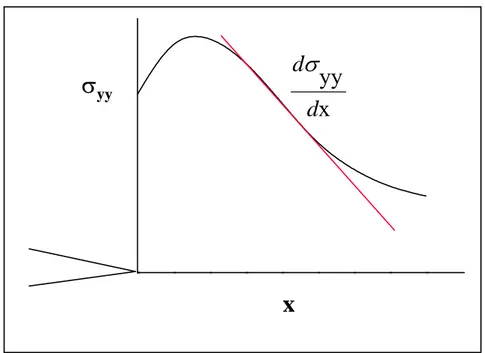
In order to solve Eq. (3-15), the conditional probability of propagation (P{P/I}) must be known in a functional form. Presently it is not possible to define a single specific function for P{P/I}, but some possible forms can be deduced from the stress distribution. If the probability of propagation is controlled by the steepness of the stress distribution, it will essentially be a function of the derivative of the HRR field, as shown in Fig. 3.7.

x

σ

_yy

d

d

σ

_yy

x

Fig. 3.7: Steepness of stress distribution in front of crack. The stress distribution can be expressed as:

) ( 1 N 1 x 2 I K yy

θ

σ

⋅ f + ⎟ ⎟ ⎟ ⎠ ⎞ ⎜ ⎜ ⎜ ⎝ ⎛ = (3-16)

where N is the strain hardening exponent.

1 N ) ( 2 I 2 N yy 1 1 x yy + ⋅ + ⋅ ⎟ ⎠ ⎞ ⎜ ⎝ ⎛ + − =

θ

σ

∂

∂σ

f K N (3-17)

It is seen from Eq. (3-17) that the steepness of the stress distribution is a combined function of the stress, angular location and the stress intensity factor. The stress and angular dependence are random parameters (independent of KI) thus causing the probability of propagation to be a

simple function of KI. If P{P/I} is only controlled by the steepness of the stress distribution,

two possible forms are evident as expressed in Eq. (3-18a) and (3-18b):

( )

⎥ ⎥ ⎥ ⎦ ⎤ ⎢ ⎢ ⎢ ⎣ ⎡ ⎟ ⎟ ⎠ ⎞ ⎜ ⎜ ⎝ ⎛ − ⋅ = 2 I K min1 K 1 1 A P/I 1 P (3-18a) and

( )

2 I K min2 K 1 2 A P/I 2 P _⎟⎟ ⎠ ⎞ ⎜ ⎜ ⎝ ⎛ − ⋅ = (3-18b)

However, since P{P/I} is a measure of an instantaneous propagation rate, it is possible that it is controlled by the change rate of the steepness of the stress distribution (Eq. 3-19).

1 N ) ( 3 I K 2 N yy 1 N 2 x yy I K _⋅ + + ⋅ ⎟ ⎠ ⎞ ⎜ ⎝ ⎛ + = ⎟⎟ ⎟ ⎠ ⎞ ⎜⎜ ⎜ ⎝ ⎛

θ

σ

∂

∂σ

∂

∂

f (19)

Eq. (3-19) implies two additional possible forms for P{P/I}, Eq. (3-20a) and (3-20b)

( )

⎥ ⎥ ⎥ ⎦ ⎤ ⎢ ⎢ ⎢ ⎣ ⎡ ⎟ ⎟ ⎠ ⎞ ⎜ ⎜ ⎝ ⎛ − ⋅ = 3 I K min3 K 1 3 A P/I 3 P (3-20a) and

( )

3 I K min4 K 1 4 A P/I 4 P _⎟⎟ ⎠ ⎞ ⎜ ⎜ ⎝ ⎛ − ⋅ = (3-20b)

The possible forms are presented graphically in Fig. 3.8. All the equations are functions growing from 0 to A, where A is a number smaller than 1. The constant A reflects the finite probability of crack arrest even in a uniform stress field, being due to a possible misorientation between the microcrack and the possible cleavage crack planes and the need to cross a grain boundary.

0 2 4 6 8 10 0.0 0.1 0.2 0.3 0.4 0.5 0.6 A = 0.5 P₁(P/I) P₂(P/I) P₃(P/I) P₄(P/I)

P(

P/

I)

K

_I

/K

_{m in}

Fig. 3.8: Comparison of the different conditional propagation probability functions in Eqs. (3-18) and (3-20) using A = 0.5 as the limiting propagation probability.

When Eqs. (3-18) and (3-20) are inserted into Eq. (3-15), the following possible forms for the total cumulative failure probability are obtained

⎪⎭ ⎪ ⎬ ⎫ ⎪⎩ ⎪ ⎨ ⎧ ⎟ ⎠ ⎞ ⎜ ⎝ ⎛ ₋ ⋅ ⋅ − − = 2 2 min1 K 2 I K 4 0 K 1 A 0 B B exp 1 f1 P (3-21a)

(

) (

)

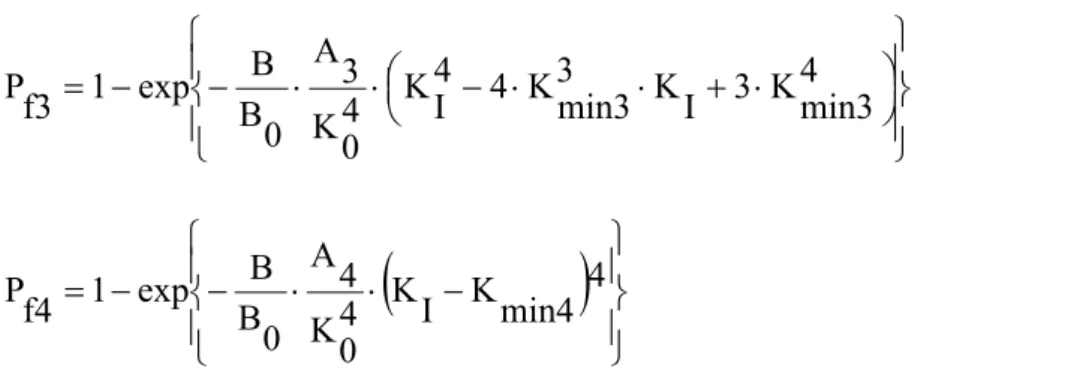
⎪⎭ ⎪ ⎬ ⎫ ⎪⎩ ⎪ ⎨ ⎧ + ⋅ − ⋅ ⋅ − − = K_I K_min2 3 K_I K_min2 3 4 0 K 2 A 0 B B exp 1 f2 P (3-21b)s

⎪⎭ ⎪ ⎬ ⎫ ⎪⎩ ⎪ ⎨ ⎧ ⎟ ⎠ ⎞ ⎜ ⎝ ⎛ _{− ⋅ ⋅ + ⋅} ⋅ ⋅ − − = 4 min3 K 3 I K 3 min3 K 4 4 I K 4 0 K 3 A 0 B B exp 1 f3 P (3-21c)

(

)

⎪⎭ ⎪ ⎬ ⎫ ⎪⎩ ⎪ ⎨ ⎧ − ⋅ ⋅ − − = K_I K_min4 4 4 0 K 4 A 0 B B exp 1 f4 P (3-21d)

The equations are compared graphically in Fig. 3.9, where Kmin refers to Kmin4.

Experimentally it is virtually impossible (would require more than 1000 tests) to tell the four expressions apart. They start clearly to deviate from each other only at very low cumulative probability values. The expression producing the most conservative estimate for the minimum fracture toughness is Pf4. 0 2 4 6 8 1 0 0 .0 0 .5 1 .0 1 .5 2 .0 P_f1 P_f2 P_f3 P_f4 9 9 % 1 %

{l

n[

1/

(1

-P

f

)]

}

0. 25

K

_I

/K

_{m in}

Fig. 3.9: Comparison of different cumulative failure probability expressions, Eq. (3-21a-d). The expressions are plotted against a normalised form of Pf4, using K0/Kmin4 = 5.

The individual parameter values used in Fig. 3.9 are presented in Table 3.1, which essentially confirms the trends seen in Fig. 3.9. The expression Pf1 is essentially identical with Pf3 and Pf2

is essentially identical with Pf4 and Pf4 yields the most conservative estimate of Kmin. For

engineering safety assessment purposes it is clearly advisable to use Pf4 to describe the

cumulative failure probability.

Pf1 A1/A4 = 0.66 Kmin1/Kmin4 = 2.28

Pf2 A2/A4 = 0.90 Kmin2/Kmin4 = 1.20

Pf3 A3/A4 = 0.60 Kmin3/Kmin4 = 2.48

Pf4 A4/A4 = 1 Kmin4/Kmin4 = 1

The above derivations are based on the assumption that the probability of cleavage initiation is less than unity. This is normal for configurations like plain and notched specimens and cracked specimens in cases where initiation is sufficiently difficult. For material conditions where initiation is simple, the probability of cleavage initiation in the case of a crack may become unity. This can occur on the so called “lower shelf” of the material. Essentially it means that all possible initiation sites are activated and initiation occurs as soon as the crack is loaded, making the initiation event independent of the load level (and subsequently independent of specimen thickness). Thus, in the case of a crack, the lower shelf toughness may be controlled purely by the probability of propagation. For plain and notched configurations, however, the probability of initiation will still be a function of load level even on the lower shelf. Therefore, a simple correlation between notched and cracked configurations may not be possible for the lower shelf material conditions.

As previously stated, the conditional probability of propagation (P{P/I}) indicates the instantaneous probability of propagation and as such it is similar to the hazard function for propagation alone. However P{P/I} does not as such constitute a hazard function, because the hazard function (like the incremental distribution) must have the units of 1/KI. Therefore,

substitution of the normalisation parameter Ke in the place of the constant A yield, corollary

to Eqs. (3-18 and 3-20), logical forms for the hazard function of propagation alone:

⎥ ⎥ ⎥ ⎦ ⎤ ⎢ ⎢ ⎢ ⎣ ⎡ ⎟ ⎟ ⎠ ⎞ ⎜ ⎜ ⎝ ⎛ − ⋅ = 2 I K min1 K 1 e1 K 1 ) I K ( P1 h (3-22a)

2 I K min2 K 1 e2 K 1 ) I K ( P2 h _⎟⎟ ⎠ ⎞ ⎜ ⎜ ⎝ ⎛ − ⋅ = (3-22b) ⎥ ⎥ ⎥ ⎦ ⎤ ⎢ ⎢ ⎢ ⎣ ⎡ ⎟ ⎟ ⎠ ⎞ ⎜ ⎜ ⎝ ⎛ − ⋅ = 3 I K min3 K 1 e3 K 1 ) I K ( P3 h (3-22c) 3 I K min4 K 1 e4 K 1 ) I (K P4 h _⎟⎟ ⎠ ⎞ ⎜ ⎜ ⎝ ⎛ − ⋅ = (3-22d)

The corresponding cumulative failure probabilities are:

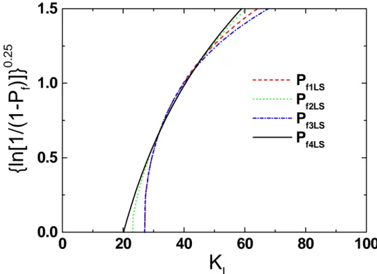
⎪⎭ ⎪ ⎬ ⎫ ⎪⎩ ⎪ ⎨ ⎧ ⎥ ⎥ ⎦ ⎤ ⎢ ⎢ ⎣ ⎡ − + ⋅ − = 2 1 K min1 K min1 K I K e1 K min1 K -exp 1 f1LS P (3-23a) ⎪⎭ ⎪ ⎬ ⎫ ⎪⎩ ⎪ ⎨ ⎧ ⎥ ⎥ ⎦ ⎤ ⎢ ⎢ ⎣ ⎡ − + ⎟ ⎟ ⎠ ⎞ ⎜ ⎜ ⎝ ⎛ ⋅ ⋅ − = 1 K min2 K min2 K I K I K min2 K ln 2 e2 K min2 K -exp 1 f2LS P (3-23b) ⎪ ⎭ ⎪ ⎬ ⎫ ⎪ ⎩ ⎪ ⎨ ⎧ ⎥ ⎥ ⎥ ⎦ ⎤ ⎢ ⎢ ⎢ ⎣ ⎡ − ⎟ ⎟ ⎠ ⎞ ⎜ ⎜ ⎝ ⎛ ⋅ + ⋅ − = 2 3 2 1 K min3 K 2 1 min3 K I K e3 K min3 K -exp 1 f3LS P (23c) ⎪ ⎭ ⎪ ⎬ ⎫ ⎪ ⎩ ⎪ ⎨ ⎧ ⎥ ⎥ ⎥ ⎦ ⎤ ⎢ ⎢ ⎢ ⎣ ⎡ + ⎟ ⎟ ⎠ ⎞ ⎜ ⎜ ⎝ ⎛ + ⋅ − ⎟ ⎟ ⎠ ⎞ ⎜ ⎜ ⎝ ⎛ ⋅ − ⋅ − = 2 3 2 I K min4 K 2 1 1 K min4 K 3 min4 K I K ln 3 min4 K I K e4 K min4 K -exp 1 f4LS P (3-23d)

Eqs. (3-23a-d) are compared in graphic form in Fig. 3.10 for an imaginary lower shelf data set with a median fracture toughness of approximately 40 (units not specified). The same trend as before for the initiation plus propagation case is seen. The expression Pf1LS is essentially

identical with Pf3LS and Pf2LS is essentially identical with Pf4LS and Pf4LS yields the most

compared to existing lower shelf data. Expression Pf2LS appears, intuitively, from the stress

distribution point of view to be most likely the correct one, but the expression Pf4LS is almost

identical in shape and slightly more conservative. Additionally, the form of Pf4 (for initiation

+ propagation) is very suitable for statistical estimation, because it is identical to a simple three parameter Weibull distribution with a fixed shape (exponent = 4). Thus, Pf4 and Pf4LS are

selected as the basis for the Master Curve scatter and size effect.

The Master Curve scatter in the case of initiation plus propagation is described optimally by Eq. (3-21d), which can be reformulated in the convenient form of a three parameter Weibull expression with the exponent fixed to 4:

⎪ ⎭ ⎪ ⎬ ⎫ ⎪ ⎩ ⎪ ⎨ ⎧ ⎟ ⎟ ⎠ ⎞ ⎜ ⎜ ⎝ ⎛ − − ⋅ − − = 4 min K 0 K min K I K 0 B B exp 1 f P (3-24)

Here, K0 equals the load level corresponding to a 63.2 % cumulative failure probability, B0 is

a freely selected normalising thickness, e.g. 25 mm and Kmin is the lower limiting fracture

toughness corresponding to zero probability of failure. The size effect, implied by Eq. (3-24), has the form:

1/4 2 B 1 B ) min K (1) IC (K min K (2) IC K _⎟⎟ ⎠ ⎞ ⎜ ⎜ ⎝ ⎛ ⋅ − + = (3-25)

The theory predicts that the size effect disappears in the lower shelf toughness range and also the scatter changes somewhat, compare Figs. 3.9 and 3.10. On the lower shelf the cumulative failure probability is described by Eq. (3-23d) which is of a somewhat more complex form than Eq. (3-24). Unfortunately, the derivation is incapable of predicting when lower shelf conditions are prevailing, thus making it difficult to decide when to use Eq. (3-24) and when to use Eq. (3-23d). Experimentally the problem can easily be solved by performing tests in

both regions. From an engineering assessment point of view, however, a conservative estimate is obtained with Eq. (3-24) also on the lower shelf.

0

20

40

60

80

100

0.0

0.5

1.0

1.5

P

_f1LS

P

_f2LS

P

_f3LS

P

_f4LS

{ln[

1/

(1-P

f

)]}

0. 25

K

_I

Fig. 3.10: Comparison of different possible cumulative failure probability expressions for lower shelf behaviour in Eq. (3-23a-d).

In the case of initiation, the resulting equations contain no approximations. The only assumption is that the initiators are independent on a global scale. In other words, it is assumed that the volume elements are independent for a constant KI. Only, if it is assumed that a certain fraction

of the crack front must experience critical initiations to cause macroscopic failure, then the result will differ from what is presented here. The only other restriction comes from the requirement that the volume elements in the x-direction must be clearly larger than the initiator size, but this requirement is effective only for the transition region where it is easily fulfilled. On the lower shelf, initiation is automatic and does not depend on the volume element size.

In the case of propagation, the resulting equations contain more uncertainties, but in this case, a conservative result has been chosen.

In the derivation of the above equations, the cleavage fracture process zone was assumed to be equal to the region of high stresses and plastic strain. The result is, however, not sensitive to the definition of the process zone as long as it is assumed that the stress and strain distributions inside the process zone correlate with KI, CTOD or J. This aspect becomes important when

4. DETERMINATION OF MASTER CURVES

The ASTM E1921-03 standard describes the determination of a reference temperature, T0 in o_{C, which characterizes the fracture toughness of ferritic steels that experience onset of}

cleavage cracking at elastic, or elastic-plastic KJc instability, or both. By definition, T0 is a

temperature at which the median of the KJc distribution from 1T size specimens will be equal

to 100 MPa√m. Static elastic-plastic fracture tests are performed on standard SEN(B) or CT specimens having deep notches (a/W= 0.5) to measure the J-integral values at cleavage fracture (denoted Jc). The test temperature (T) and configuration of all specimens must be

identified. The test temperature should be selected in the lower part of the ductile-to-brittle region as close as possible to the eventual T0. The standard requires a minimum of six

replicate tests which meet the crack front straightness tolerances, the limits on ductile tearing prior to cleavage, the size/deformation limits, etc. It is also possible to use miniature specimen sizes in the fracture toughness test. For example, using test specimens of section 5x5 mm2 needs 12 validated tests (Table 5-3). The J-integral values at fracture are converted to their equivalent units of stress intensity factor using:

1) -(4 , m MPa 1₋

_ν

2 = c Jc EJ K

where E denotes the elastic modulus and ν the Poisson’s ratio of the material. The maximum

KJc capacity of a specimen is restricted to:

2) -(4 , ) 1 ( 2 0 (limit) _ν σ − = M Eb K Y Jc

where σY is the material yield strength at the test temperature and b0 the specimen remaining

ligament. The standard sets M = 30 in order to assure that the SSY condition prevails in the test specimen. KJc data that exceed this requirement may be used in a data censoring

conducted on other than 1T specimens, the measured toughness data should be size-corrected to their 1T equivalent according to

[

20

]

(4-3) 20 4 1 1 x 1 , B B K K T Jc(x) T) Jc( ⎟⎟ ⎠ ⎞ ⎜⎜ ⎝ ⎛ − + =

where B1T is the 1T specimen size (25 mm) and Bx the corresponding dimension of the test

specimen. In Eq. (4-3), 20 MPa√m represents the minimum (threshold) fracture toughness adopted for ferritic steels addressed by the standard.

The ASTM E1921-03 standard adopts a three-parameter Weibull model to define the relationship between KJc and the cumulative failure probability, Pf. The term Pf is the

probability for failure at or before KJc for an arbitrarily chosen specimen taken from a large

population of specimens. By specifying two of the three Weibull parameters, the failure probability has the form:

4) -(4 . exp 1 4 min 0 min ⎟ ⎟ ⎠ ⎞ ⎜ ⎜ ⎝ ⎛ ⎥ ⎦ ⎤ ⎢ ⎣ ⎡ − − − − = K K K K Pf Jc

Here, the Weibull distribution shape has been assigned a value of 4 derived from theoretical arguments. For ferritic steels with yield strengths ranging from 275 to 825 MPa, the cumulative probability distribution of the fracture toughness is independent of specimen size and test temperature, when Kmin is set as 20 MPa√m. The scale parameter K0 is the data-fitting

parameter. K0 corresponds to 63% cumulative probability. When using the maximum

likelihood statistical method of data fitting, KJc and K0 are equal, and pf is 0.632. The

following equation can be used for a sample that consists of six or more valid KJc values in

order to evaluated K0. 5) -(4 , 20 ) 20 ( 14 1 4 (i) 0 + ⎥ ⎥ ⎦ ⎤ ⎢ ⎢ ⎣ ⎡ − =

∑

= N i Jc N K K

where N denotes the number of valid tests (six minimum). Note that K0 can also be evaluated

E1921-The estimated median (50% probability) KJc value, assuming pf = 0.50 in Eq. (4-4), of the

population at the tested temperature can be obtained from K0 as expressed in Eq. (4-6):

6) -(4 . 20 ) 20 ( 9124 . 0 ₀ (med) = K − + K_Jc

The Master Curve is defined as the median (50% probability) toughness for the 1T specimen over the transition range for the material. Based on fitting to test results, the shape of the Master Curve for the 1T specimen is described by Eq. (4-7):

[

0019( )

]

. (4-7) exp 70 30 ₀ (50%) . T-T K_Jc = +

The lower-bound (5% probability) and upper-bound (95% probability) curves can also be set up. These three curves are given by the following expressions:

[

0019( )

]

. (4-8) exp 8 . 37 4 . 25 ₀ (5%) . T-T KJc = +

[

0019( )

]

. (4-9) exp 2 . 102 6 . 34 ₀ (95%) . T-T K_Jc = +

Where, KJc is in MPa√m and T and T0 in oC.

Finally, the reference temperature T0 (oC), for which KJc is 100 MPa√m, is obtained from the

following expression: 10) -(4 . 70 30 ln 019 . 0 1 (med) 0 ⎥ ⎦ ⎤ ⎢ ⎣ ⎡ − − = KJc T T

The reference temperature T0 should be relatively independent of the test temperature that has

been selected. Hence, data that are distributed over a restricted temperature range, namely T0

± 50 oC, can be used to determine T0. This temperature range together with the specimen size

requirement, Eq. (4-2), provides a validity window, where test results can be obtained, as shown in Fig. 4.1.

Note that the Master Curve methodology describes the cleavage fracture toughness of the material under high constraint conditions for which the single parameter characterization of

the material toughness (KJc) holds. Indeed, adoption of a three parameter Weibull distribution

to describe measured KJc-values, with a geometry independent value of K0, theoretically

requires that SSY conditions prevail at fracture in each of replicate test specimens used to compute the statistical estimate for K0 and thereafter T0. Moreover, the ASTM E1921 standard

does not require testing of 1T size specimens. It is allowed to use Charpy size fracture specimens (W= B= 10 mm, a/W= 0.5) and convert the results to 1T equivalent values using Eq. (4-3). This is a major advantage of the MC methodology, having in mind the severe limitations which exist on material availability in nuclear irradiation embrittlement studies. The ASTM procedure includes limits relative to specimen size and KJc-values through Eq.

(4-2). Indeed, the M= 30 value has been selected largely on the basis of experimental data sets to ensure the existence of the SSY condition at fracture of the replicate test specimens. The connection between T0 and the crack-tip constraint become exceedingly complex once SSY

conditions begin to breakdown under increasing load. This issue will be discussed in section eight of this report.

-50 0 50 0 50 100 150 SIZE ADJUSTED CVN PC TYPE DATA M = 30 5 % 95 %

K

JC

[M

P

a

√

m]

T - T

0

[

o

C]

4.1. Comparison of Master Curve K

JC

and ASME K

Ic

It is illustrative to compare the master KJc curves with the ASME KIc curves. The ASME

Section XI Code includes two reference curves, KIc and KIa, that give conservative estimates

of fracture toughness versus temperature. The KIa–curve is based on the lower bound of crack

arrest data and the KIc–curve is based on the lower bound of static initiation critical KI values

as a function of temperature. These curves are given in the Code as a function of a reference temperature, RTNDT, which is determined through drop weight and Charpy test results.

According to the Code, RTNDT is defined as the higher of the following two cases

(i) The drop weight NDT.

(ii) 33oC below the minimum temperature at which the lowest of three Charpy results is at least 68 J.

The ASME reference curves have the following forms as a function of RTNDT

[

0026( 89)

]

, (4-11) exp 355 . 1 4 . 29 + + = _NDT Ia . T-RT K

[

0036( 56)

]

, (4-12) exp 084 . 3 5 . 36 + + = NDT Ic . T-RT K

where K in MPa√m and RTNDT in oC.

It should be noted that RTNDT is not determined directly from fracture toughness tests, but

from Pellini and Charpy test (which are conducted on notched specimens under dynamic loading). On the contrary, the reference temperature T0 in the Master Curve methodology is

determined directly from fracture tests on standard cracked specimens.

A comparison between the Master Curves and the ASME KIC reference curve is shown in

Fig. 4.2. The material is a specially heat treated A533 GB to study fracture behaviour of an aged reactor pressure vessel under a cold over-pressurization scenario, [Sattari-Far, 2004a]. The T0 and RTNDT values were 30 oC and 72 oC, respectively.

A Master Curve analysis of the original data of the ASME KIC reference curve shows that the

ASME KIC curve corresponds practically to the same degree of confidence as a 5 % Master

Curve for low temperatures. This comparison is also shown in Figs. 8.18 and 8.21 and will be discussed in section 8.6 of this report.

Fig. 4.2: Cleavage fracture toughness based on the Master Curves and ASME KIc curve for a specially heat treated A533 GB steel, [Sattari-Far, 2004a].

0 50 100 150 200 250 -50 0 50 100 150

Uniaxial clad beam

Biaxial clad beam

SEN(B), a/W= 0.1 SEN(B), a/W= 0.5 5% Master Curve (B= 25 mm) 50% Master Curve (B= 25 mm) ASME KIc (RTndt= 72 o_C) K Jc , K Ic [MPam 0.5 ] Temperature [ oC]