2016:21 The effect of a glaciation on East Central Sweden: case studies on present glaciers and analyses of landform data

(1)

Research

The effect of a glaciation on East Central

Sweden: case studies on present glaciers

and analyses of landform data

2016:21

Authors: Per Holmlund,

Caroline Clason Klara Blomdahl

(2)

(3)

SSM perspective

Background and objectives

The Swedish Radiation Safety Authority reviews and assesses applica-tions for geological repositories for nuclear waste. When assessing the long term safety of the repositories it is important to consider possible future developments of climate and climate-related processes. Espe-cially the next glaciation is important for the review and assessment for the long term safety of the spent nuclear fuel repository since the presence of a thick ice sheet influences the groundwater composition, rock stresses, groundwater pressure, groundwater flow and the surface denudation. The surface denudation is dependent of the subglacial temperatures and the presence of subglacial meltwater. The Swedish Nuclear Fuel and Waste Management Company (SKB) use the Weich-selian glaciation as an analog to future glaciations. Thus, increased understanding of the last ice age will give the Swedish Radiation Safety Authority (SSM) better prerequisites to assess what impact of a future glaciation might have on a repository for spent nuclear fuel.

This report compiles research conducted between 2008 and 2015 with a primary focus on 2012-2014. The primary aim of the research was to improve our understanding of processes acting underneath an ice sheet, specifically during a deglaciation.

Results

Based on the results of studies on present day High Alpine glaciers, the Antarctic and Greenland ice sheets, and glacial geomorphological map-ping from land and marine-based data in the Gulf of Bothnia, we have gained an insight into how future glaciations may affect the northeast coast of Uppland, eastern Sweden. Evidence of ice streaming over a large distance in the Gulf of Bothnia, including the presence of numer-ous glacial lineations of varying scale, contests to a period of fast basal sliding during the Late Weichselian deglaciation. This suggests that there would have been a degree of erosion at the ice sheet bed during this time. These results have been taken into account in SSM:s reviews of SKB:s post-closure safety analysis, SR-Site, for the proposed reposi-tory at Forsmark.

The evidences for a Baltic Ice Stream are linked to the long term exist-ence of the Gulf of Bothnia and the Baltic. Unfrozen soft sea bed sedi-ments allowed a fast sliding speed at a stage of glacier advance and the bed remained wet all through the glaciation.

Need for further research

The marine-based data in the Gulf of Bothnia show indications of major landslides in glacial deposits. They might represent one or several earthquakes in connection to the sudden load off during the deglacia-tion. However, there are no seismic soundings carried out at the site so evidences for this suggested origin are lacking. Further research is thus necessary to increase the understanding of the significance of

(4)

these structures. Knowledge of any post-glacial earthquakes that have or may possibly occur in the vicinity of a possible final repository for spent nuclear fuel is of high interest for SSM in the continued review of the application for a repository since large earthquakes may induce secondary fault movements in the final disposal volume which could damage deposited canisters.

Project information

Contact person SSM: Lena Sonnerfelt and Carl-Henrik Pettersson Reference: SSM 2010-1454

(5)

2016:21

Authors: Per Holmlund, Caroline Clason, Klara Blomdahl; Stockholms Universitet, Stockholm, Sverige

The effect of a glaciation on East

Cen-tral Sweden: case studies on present

glaciers and analyses of landform data

(6)

This report concerns a study which has been conducted for the Swedish Radiation Safety Authority, SSM. The conclusions and view-points presented in the report are those of the author/authors and do not necessarily coincide with those of the SSM.

(7)

Summary

The presence of an ice sheet can exert numerous influences on the ground beneath; the weight of the overlying ice can force isostatic adjustments, and meltwater at an ice sheet bed can affect groundwater flow, ice velocity and the potential for erosion of the substrate. Collecting data on ice temperature, ice velocities, hydrology, ice geometry and meteorological conditions contributes to improving knowledge of physical processes associated with glaciation. The above-mentioned variables can be explored in contemporary ice sheet and glacier settings, but in order to understand past glaciations proxy data from glacial geomorphology must be also be applied. In this report we discuss the analysis of glacial geomorphological data from the northern Stockholm Archipelago and the sea floor of the Gulf of Bothnia, in addition to temperature and geometry changes of contemporary Swedish glaciers.

Studies on a selection of glaciers in High Alpine Sweden reveal that though the temperature distribution adjusts to changes, the speed of change cannot match a quick recession as was recorded during the deglaciation of the Weichselian Ice Sheet. The ice remained cold in analogy with the present Greenlandic Ice Sheet. The colder Antarctic environment is more in analogy with the maximum phase of the Weichselian glaciation. Basal temperature conditions reflect long term changes and are thus more influenced by the maximum phase than by variations in climate during deglaciation. At a late stage of deglaciation, meltwater may have warmed up bed temperatures. Mapping of bathymetric data provides evidence of significant subglacial water pathways and fast flowing ice along the east coast of Sweden, with further evidence for Baltic Ice Stream onset on the present day

Ångermanland-Västerbotten coast during the Late Weichselian. The existence of a Baltic Ice Stream has been shown through modelling

experiments to be a necessity to reproduce the Last Glacial Maximum extent in the Baltic sector of Scandinavian Ice Sheet, as inferred by the

geomorphological record. However, we believe that an ice shelf or a frozen patch over Åland would be necessary to sufficiently reduce ice flow and thinning in this region, and prevent premature marginal retreat.

The geomorphological landform record, with an impressive array of meltwater channels and eskers of a multitude of spatial scales, suggests that meltwater was plentiful in the Baltic/Bothnian sector during deglaciation. A numerical model was thus used to simulate the Weichselian evolution of the ice sheet and its sensitivity to surface meltwater inputs. The proportion of basal sliding that can be attributed to surface meltwater-enhanced basal sliding varies over space and time, and results of ice sheet modelling

highlight the difficulty of implementing the surface meltwater effect through simple parameterizations. This stresses the importance of continued

development of physically-based models of surface-to-bed meltwater transfer, needed to better simulate the spatial and temporal variability of

(9)

hydrology and dynamics, and their response to changes in climate and meltwater production, within ice sheet models.

The primary aim of this study was to improve our understanding of

processes acting underneath an ice sheet, specifically during a deglaciation. Based on the results of studies on present day High Alpine glaciers, the Antarctic and Greenland ice sheets, and glacial geomorphological mapping from land and marine-based data in the Gulf of Bothnia, we have gained an insight into how future glaciations may affect the northeast coast of

Uppland, eastern Sweden. Evidence of ice streaming over a large distance in the Gulf of Bothnia, including the presence of numerous glacial lineations of varying scale, contests to a period of fast basal sliding during the Late Weichselian deglaciation. This suggests that there would have been a degree of erosion at the ice sheet bed during this time.

The evidences for a Baltic Ice Stream are linked to the long term existence of the Gulf of Bothnia and the Baltic. Unfrozen soft sea bed sediments allowed a fast sliding speed at a stage of glacier advance and the bed remained wet all through the glaciation. Thus there are good reasons to assume that coming glaciations will act in a similar manner as the Weichselian glaciation did.

(10)

Sammanfattning

Ett landskap som är täckt av en inlandsis påverkas på många sätt; isens tyngd orsakar isostatiska rörelser, dess smältvatten påverkar grundvattenrörelser och isen kan erodera underlaget. Genom att studera dessa processer i nutid och spår från dåtid ökar vi kunskapsläget kring en inlandsis inverkan på en miljö. I detta arbete har vi studerat relevanta processer som pågår på svenska glaciärer idag samt de spår som den senaste skandinaviska inlandsisen har lämnat i Stockholms norra skärgård samt i Bottenhavet.

Glaciärstudien har främst handlat om hur temperaturfördelningen i isen förändras i takt med kraftig nettoavsmältning och därmed orsakar en förändring i glaciärens geometri. Det visar sig att temperaturförhållandena förändras i takt med avsmältningen, men inte tillräckligt snabbt för att kunna matcha en mycket snabb avsmältning såsom det antas ha skett vid

deglaciationen av Weichselnedisningen. Det innebär att isen förblev

kallgradig under deglaciationen, trots att det var förhållandevis varmt klimat. Den nuvarande grönländska inlandsisen är en god analog till

deglaciationsläget, medan den Antarktiska inlandsisen är mer lik Weichselisens maxskede. De basala temperaturerna under en inlandsis beskriver förhållanden som verkat under mycket lång tid. Ett maxskede av en glaciation sätter därmed ett större avtryck i den basala temperaturen än vad klimatsvängningar under en deglaciationsfas gör. I ett sent skede av deglaciation kan dock smältvatten ha bidragit till en viss uppvärmning av underlaget.

Sammanställda bottentopografiska data från svenska ostkusten och Bottenhavet visar tydliga spår av snabbt isflöde och stor inverkan av smältvatten under Weichselnedisningen. Det framgår med tydlighet att det har funnits en Baltisk isström som kan följas från Höga kusten ner till Ålands hav. Modellförsök visar också att det måste ha funnits en sådan isström för att isen ska kunna uppnå den utbredning som den hade vid olika tidpunkter under glaciationen. Vi tror att geografiska olikheter i

bottentemperaturförhållanden har bidragit till hur deglaciationsförloppet har gått till. Samtidigt som en isström har gått genom Södra Kvarken och Ålands hav har sannolikt isen varit bottenfrusen vid nuvarande Åland.

Modellförsöken visar att deglaciationsförloppet annars skulle gå för snabbt och ge en isfrontsgeometri som inte överensstämmer med rådande

uppfattning.

De geomorfologiska spåren i främst bottentopografidata visar på en rikedom av smältvattenrännor och åsar av olika åldrar. Spåren vittnar om stora smältvattenmängder under degalaciationsskedet. En numerisk modell användes därför för att simulera Weichselisen och dess känslighet för smältvatteninjektioner i underlaget. Den basala glidningen påverkas mycket konkret av smältvattnet från isytan och processen är svår att modellera eftersom snabba slumpmässiga förändringar kan ge stor effekt under ett deglaciationsskede, vilket har tydliggjorts vid fältstudier på Grönland. De bottentopografidata som har insamlats från Bottenhavet beskriver ett

avsmältningsförlopp där vi kan följa tidsmässiga och rumsliga förändringar i vattenflödet som på ett väsentligt sätt ökat vår kunskap kring hur en

(11)

Huvudmålet med denna studie har varit att öka vår kunskap kring processer som påverkar underlaget under en glaciation med speciellt fokus på

deglaciationsskedet. Med stöd av våra studier av nutida glaciärer och

inlandsisar samt geomorfologiska data från land och havsbotten har vi fått en ökad insikt i hur en kommande nedisning kan påverka miljöerna vid norra Upplandskusten. Den isström som har gått från Bottenhavet ner till Ålands hav har lämnat mycket tydliga spår i havsbottnen och rimligen medfört en hög grad av erosion. Väster om den djupränna som isströmmen har gått i är de glaciala spåren också tydliga, men där är erosionen svårare att kvantifiera. Beläggen för att det har funnits en baltisk isström är kopplade till existensen av Bottenhavet och Östersjön. När en inlandsis avancerar ut över dessa sedimenttäckta havsbottnar så har isrörelsehastigheten ökat väsentligt vilket har givit förutsättningarna för ett effektivt isflöde längs detta nord-sydliga stråk och genom deformationsvärme har området förblivit bottensmältande genom glaciationen. Det finns därmed all anledning att tro att kommande glaciationer kommer att ha ett liknande utvecklingsmönster som

Weichselnedisningen hade.

1. Introduction

This report compiles research conducted between 2008 and 2015 with a primary focus on 2012-2014. The aim of this report is to investigate

processes occurring at the interface between an ice sheet and its substrate. As part of the research we performed numerical modeling, field studies and a range of data analyses, including the mapping of glacial geomorphological landforms from remotely sensed data. Fieldwork was conducted both on present-day glaciers in Northern Sweden, and in the Northern Stockholm Archipelago. We also planned to extend a radar study of bed topography in East Antarctica, but it was not possible within the time framework of this study. However, data already sampled during the Japanese Swedish

Antarctic Expedition (JASE)(Fujita et al. 2011) are used in the discussion to explore the effect of present ice sheets on their bed and landforms.

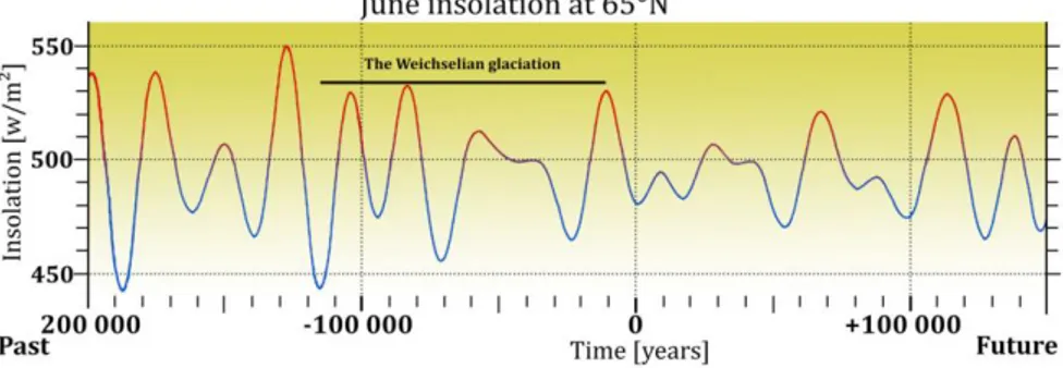
Our study of glaciers in Northern Sweden focus on how the thermal regime of glaciers respond to major geometry changes forced by climate. These glaciers are all situated in a region typified by the presence of permafrost, where glaciers ae normally “warm” spots. The glaciers in our study area are polythermal, which means that they consist of ice both at pressure melting point and ice below freezing. These glacier studies contribute to our understanding of the interaction between climate and the internal ice temperature in a glacier. Research conducted in the archipelago involved glacial geomorphological mappings on numerous islands, which was later extended by bathymetric data from the Swedish sector of the Gulf of Bothnia. The bathymetric data came to us late in this process and is thus not fully analyzed herein. The Gulf of Bothnia is surprisingly rich in traces from the Weichselian glaciation and landforms predating the glaciation also exist. The Weichselian glaciation is used by Svensk Kärnbränslehantering AB (SKB) as a typical glaciation in their research on possible external stresses on a storage for nuclear waste at Forsmark. Figure 1.1 shows values of solar

(12)

insolation calculated from past and future variations in accordance with the so called Milankowitch cycles. These cycles show when warming and cooling events occurs but they do not show the actual response of the climate system.

Figure 1.1. Calculated variations in insolation from the sun based on the

Milankowitch theory. It includes variations in Earth orbit and angle changes in earth axis. The figure shows past and future variations at 65 degrees north (Berger and Loutre 2002).

The research described herein focusses on glacial processes, with specific focus on meltwater flow, glacial erosion and glacial morphology. The processes investigated here are not well understood and thus we are

advancing on existing scientific knowledge. We are using mountain glaciers as laboratories upon which to examine contemporary processes, East Central Sweden as our area of specific interest, and Antarctica and Greenland as analogues for a glaciation in Scandinavia, with numerical modelling to evaluate ice sheet sensitivity to external forcings. By combining results from these scientific and geographic fields our understanding of how an ice sheet affects its substratum during a cycle of glaciation is improved. A glaciation will not only affect the ground by direct glacial processes, but also by periglacial processes like permafrost. The latter is herein only reviewed from other studies.

1.1. Permafrost

Permafrost is widely found in the Sub and High Arctic (King 1984, Harris et al. 2001, Harris et al. 2003). Discontinuous permafrost occurs at annual mean temperatures between -2°C and -5°C, while under colder conditions, permafrost is continuous. Lakes and rivers act as heat sources and constitute warm spots within permafrost areas; so called taliks. Except for the inner part of Greenland, the ground in the High Arctic and Sub Arctic is

characterized by summer melt and the formation of an active layer, normally up to a meter thick.

There are several parameters influencing the occurrence of permafrost, such as climate, substrate type, vegetation, exposure, groundwater flow and geothermal heat flux. Climate forcings do not only include meteorological variables such as temperature, precipitation, and wind speed, they also include large-scale temporal and spatial effects such as the seasonal

(13)

distribution of rain and snow, occurrence of temperature inversions and the influence of topography. But local meteorological conditions can deviate significantly from regional patterns.

Global warming inevitably causes permafrost thawing. Most research on permafrost focusses on changes in its distribution and in the thickness of the active layer. Carbon and methane fluxes from the thawing ground to the atmosphere have the potential to boost future atmospheric warming. A study of past permafrost distribution on the North American continent was carried out by French and Millar (2014). They mapped fossil ice wedges, patterned ground and other landforms associated to permafrost, eluding to a broad permafrost extent of along the margin of the ice sheet during the last maximum of the Laurentide Ice Sheet. Similar mappings have been

conducted in Europe, with fossil ice wedges in Skåne dated to the Younger Dryas (Svensson 1964, 1974). Ice wedges are believed to form at annual mean temperatures lower than -6- -8°C (French and Millar 2014).

Physical data on permafrost at drill sites are compiled by Global Terrestrial Network for Permafrost (GTN-p). The majority data points are from shallow holes with depths up to 20 m. Deep drilling has been carried out for the purpose of prospecting for oil or gas, and to a lesser extent for scientific purposes. There are a relatively large number of deep drill holes with depths exceeding the permafrost thickness. Clow (2014) made an analysis of data from 23 boreholes in Alaska for the period 1973-2013. The drill holes were between 227 and 884 m deep and the permafrost depth varied between 210 and 400 m, though most of them had depths around 300 m. The geothermal gradient at the sites were dependent on type of bedrock and climate impact, and varied between 2 and 4°C/100 m (Clow 2014). At some sites it showed variations with depth, which may be an effect on past climatic changes. Between1998-2002 an EU funded project named Permafrost and Climate in Europe (PACE) was conducted (Harris et al. 2001, 2003). 100 m deep drill holes in rock were equipped with temperature sensors and have been monitored since. There are about 10 sites from Svalbard in the north to the Sierra Nevada in the South, and all indicate a warming trend since

installation.

In April 2000, one 100 m and two 15 m holes were drilled into the bedrock close to Tarfala Research Station (Harris et al 2001, Isaksen et al 2001). One 15 m deep hole was drilled by the station at 1130 m above sea level (a.s.l.) at the site of the weather station which has been operating during summer since 1946 and automatically all year round since 1965. At Tarfalaryggen, a saddle area at 1550 m a.s.l., one 100 m and one 15 m deep borehole were drilled and a weather station was erected. The annual mean air temperature is -6°C, the annual precipitation rate is about 500 mm and the permafrost depth is estimated to exceed 300 m. The measured borehole base (100m) temperature was -2.7°C. At Tarfala Research station the annual mean air temperature is -3.9°C, the annual mean precipitation is about 1000 mm and the permafrost is discontinuous. The top 7 m at the site consists of a till cover and the bedrock beneath showed below freezing temperatures when the hole was drilled, but successive surveys have since recorded zero degrees. (Isaksen et al 2001, Isaksen et al 2007).

(14)

1.2. Temperature in ice

The temperature within glaciers is more complicated to estimate than the temperature in the ground. Glaciers are moving and snow and temperate ice is permeable to meltwater which releases latent heat. The temperature of ice influences its viscosity, such that an ice body at zero degrees deforms 40 times quicker than a corresponding ice body at -20°C. The temperature also influences the extent to which liquid water is present within or at the base of a glacier, and further influences ice flow by enhancing sliding between the ice and the bed. The ice temperature is thus of fundamental importance for discussions on how a glacier interacts with and affects its substrate. Ice is a relatively bad conductor of heat. A sinusoidal temperature wave on an ice body needs 5.5 months to reach a depth of 10 m (Cuffey and Paterson 2010). If climate slowly changes, a glacier will adapt its thermal regime to a new situation, but in the case of quick changes the temperature regime will be out of balance with the climate. When the Weichselian Ice Sheet retreated over Uppland the recession rate was on the order of 300 m/year indicating a melt rate (thinning via melting of glacial ice) of more than 10 metres per year. This means that only the very surface of the retreating ice was affected by the warm Holocene climate, while the majority of the ice column

remained cold.

There have been some studies on how the temperature regime changes within a glacier with a changing climate. On McCall Glacier in Alaska Delcourt et al (2013) made an analysis of the effect of a gradual change in Equilibrium Line Altitude (ELA) as had been recorded over the last 50 years. The measurements of temperature distribution showed a significant lag in their response. The change in ELA caused a cooling of the glacier as the accumulation area gradually turned into an ablation area, thus no latent heat was released within the ice due to refreezing processes (Delcourt et al 2013). In this report we describe how the thermal regime of selected Swedish glaciers has responded to both changes in climate and geometry.

1.3. Traces of past glaciations in East Central Sweden

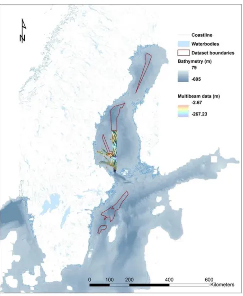
Mapping of landforms included field surveys on a number o islands in the North Stockholm Archipelago and analysis of remotely sensed bathymetric data. The bathymetric data, collected by multibeam, are completely new to the scientific community. In Figure 1.2 the areas of bathymetric data used within our reseach are highlighted. The colored area is used specifically for this project while datasets indicated by red lines area areas for which mapping was conducted from multibeam data available at Sveriges

Geologiska undersökning (SGU). All data are from Swedish waters and have been delivered by Sjöfartsverket. In addition we have made use of seismic data (not indicated in figure 1.2) provided by, and in cooperation with SGU.

(15)

Figure 1.2 The Bathymetric data used for this study. Background bathymetry is from the Baltic Sea Bathymetry Database at 500 m resolution, multibeam data depicted is sourced from Sjöfartverket at 5 m resolution, with areas outlined in red mapped from multibeam data available at SGU. The multibeam data depicted were specifically provided for this study, and are described in more detail in chapters 4 and 5.

(16)

2. Spatial and temporal changes of size

and thermal regime of alpine

Glaciers

2.1. Response to climate change

Glaciers are by definition very good climate indicators as changes in their size and form are forced by climatic conditions. The exponential relationship between ice thickness and ice flow results in responses to small climatic perturbations. However, the response time of Swedish subarctic glaciers are typically 50-100 years (Holmlund 1988a, 1993), so observed length changes are results of not only present day climatic changes, but also climate

fluctuations over the last century. Most Swedish glaciers have a polythermal temperature regime, meaning that they are in part temperate and in part cold, or below the pressure melting point (Blatter and Hutter 1991, Holmlund and Eriksson 1989, Pettersson et al. 2003). The relative extent of cold and temperate ice differs between glaciers due to local climatic effects. In the simplest case the glaciers are temperate in their accumulation area and more or less cold in the ablation zone. But in permafrost regions the temperature regime is complicated by ice cored moraines and perennial snow fields which are physically linked to the glaciers, and thus influence their response to climatic fluctuations (Holmlund 1998).

In the springs of 2008-14 radar soundings were performed and more than 80 glaciers were surveyed, some glaciers in much detail and others by a single length profile. The number of glaciers studied make up more than a quarter of all glaciers in Sweden, but the selection of glaciers is biased to relatively large glaciers with historical scientific information on size changes (Bolin 2014). In this report data from these studies are presented and analyzed, including examples of extreme physical settings and responses.

The temperature distribution in a glacier is determined by the pattern of snow accumulation, the rate of mass turnover and the air temperature (Pettersson et al. 2003). In the wintertime the surface of the glacier is cooled to a certain degree and a certain depth. In the spring when melting occurs, meltwater penetrates the snow pack and efficiently raises the temperature to the melting point via energy released from refreezing of meltwater. In the accumulation area of a glacier this process will also warm up past years snow (firn). If meltwater meets an ice surface within or below the snow pack the meltwater cannot penetrate beneath this surface so it refreezes as

superimposed ice or flows horizontally across the ice surface. Cooling from the winter thus remains in the ice and over time forms a permanent below freezing point layer. In glaciers with low ice mass turn over, the thickness of this layer is large and in glaciers with a high rate of mass turn over this layer is shallower. A typical value for the cold surface layer depth in Swedish glaciers is 100 m in dry areas and 10-20 m in wetter areas. On glaciers originating from multiple accumulation areas there can be significant spatial variation in thermal conditions.

(17)

If a polythermal glacier thins its average temperature is believed to decrease (Pettersson et al. 2003), which may result in small glaciers freezing on to their bed, preventing them from sliding. The glacier may become steeper by this process, but at the same time could hinder the transportation of ice mass to the glacier front. This could in turn cause a dramatic change in areal extent. In the event of a shift to a more favourable climate, a small, steep glacier can reach pressure melting point at the base and thus make a dramatic quick advance of its front position (Murray et al 2000). Glaciers in dry environments may become stagnant, yet remain for a relatively long time. The temperature at the base of such ice bodies is low, due to a lack of melting and water penetration through the ice, and due to the relatively low annual temperatures in the Swedish mountains.

Topography is very important both for the mass balance of and the temperature distribution within a glacier. A steep headwall will provide a glacier with snow to ensure net accumulation in the upper reaches of the glacier. This could also result in a sufficiently deep snow/firn layer in order for the ice to be formed at the pressure melting point. If there is no headwall or a gap in the headwall, much less snow will be accumulated and ice temperatures and thus ice velocities will be low.

2.1.1. Data

Eighty glaciers were studied during several field campaigns distributed over seven years. A continuous-wave stepped-frequency (CWSF) radar system was operated from a helicopter platform with its geographical position sampled by a GPS receiver. The radar soundings were performed in late spring (April) when it is still cold but days are bright and long. The radar system consists of a Hewlett Packard Network Analyzer (8753ET) (Hamran and Aarholt, 1993, Hamran et al. 1995) and log-periodic antenna. The system gives full control of the transmitted bandwidth, but for our purposes we chose to use a center frequency of 820 MHz and a bandwidth of 100 MHz. The radar acquired ~2 records per second giving a trace distance of ~10 m, and the collected data was transformed to the time-domain using inverse Fourier transform with no further filtering. This radar system has been successful in imaging the thermal regime of polythermal glaciers (Holmlund et al. 1989, Björnsson et al, 1996, Pettersson et al. 2003), and the mapped boundary between the cold surface layer and temperate ice is within a accuracy of ±1 m (Pettersson et al., 2003).

The results of these radar studies depict large differences in thermal structure between individual glaciers. All glaciers are below freezing point at their terminus, but the up-glacier longitudinal extension of this cold zone varies significantly; from a few tens of metres up to a kilometer. This highlights the differences in their respective response to climatic changes. A glacier which is frozen to its bed for several hundreds of metres cannot easily advance, while a more temperate glacier, aided by water at the bed, can. Therefore very few glacier advances have been reported from Sweden during the last century, and would require a period of significant cooling or increased precipitation in order to build mass and advance.

(18)

2.2. A case study of temperature and geometry

changes of five Swedish glaciers

In this chapter we describe the changing geometry and thermal regime of a sample of five Swedish glaciers over time. Changes in geometry were observed from the creation of digital terrain models from data obtained through aerial photography, while changes in the thermal regime were surveyed using ice penetrating radar.

2.2.1. How do Swedish glaciers respond to warming?

Annual variations in glacier surface elevation result from winter accumulation and summer melting, but under unchanging climatic

conditions result in the same net ice volume from year to year. While surface expression of response to climatic changes can be immediate, ice volume and terminus response is much slower. A time series of ice surface change of a typical Swedish glacier affected by a step-increase in temperature would show an adaption migrating from the upper reaches of the glacier to the terminus. When the terminus has adjusted to a new climatic situation, a new steady state is achieved. This way of adjusting the geometry is also

applicable at ice sheet scale, though the response time is much longer; up to thousands of years. Geometry changes thus help to tell us how close a glacier is to a steady state or whether a glacier mass balance is unhealthy.

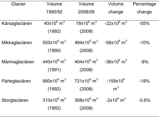
Table 1. Total volume change (106 m3) during 1990-2009 for selected Swedish glaciers. Volume changes for Kårsaglaciären were calculated from data in Rippin et al., 2011. Glacier Volume 1990/92 Volume 2008/09 Volume change Percentage change Kårsaglaciären 40x106 m3 (1992) 18x106 m3 (2009) -22x106 m3 -55% Mikkaglaciären 550x106 m3 (1990) 494x106 m3 (2008) -56x106 m3 -10% Mårmaglaciären 440x106 m3 (1991) 404x106 m3 (2008) -36x106 m3 -8% Pårteglaciären 880x106 m3 (1992) 721x106 m3 (2008) -159x106 m3 -18% Storglaciären 310x106 m3 (1992) 308x106 m3 (2008) -2x106 m3 -0.6%

(19)

2.2.2. Ice surface elevation surveys

Digital elevation models (DEMs) were used in this study to quantify the long-time volume variations on Pårteglaciären, Mårmaglaciären and Mikkaglaciären. By calculating the difference between two or more DEMs separated in time, it is possible to obtain a measure of the elevation change. This method is appropriate for long-term studies of glacier changes

(Klingbjer and Neidhart, 2006). The DEMs allow calculations of the mean net mass balance, although the results do not provide any information on annual variations in accumulation or ablation. The correlation between traditional mass balance measurements and geodetic mass balance calculations have been found to be generally good in several studies (Holmlund, 1987; Krimmel, 1999; Klingbjer and Neidhart, 2006).

Elevation datasets from the National Land Survey of Sweden were used to create the DEMs. The elevation was calculated digitally from aerial photos from around 1960, 1990 and 2008 taken at the end of the melt season. From the DEMs the volume changes were calculated for the time periods

available. The original elevation data were imported and converted to raster format in ArcGIS. The elevation rasters were subtracted from each other to obtain the change in elevation between the datasets. Rasters of the surface change were cropped based on the extent of each glacier for each year and the area changes, volume changes and net surface lowering were calculated using the Zonal Statistic Tool.

The bottom topography of the tongue of Mikkaglaciären was mapped using a 8 MHz pulsed Mark II radar with dipole antennae, and the data recorded on photographic film, in May 1983 (Holmlund 1986). Mårmaglaciären was mapped using the same equipment and method in 1984 and 1987. The profiles were matched to maps constructed based on aerial photographs from August 1980 and August 1978 respectively. As surface maps and ice

thickness surveys are close in time the bottom maps are believed to be reliable. The bed of Storglaciären was mapped in 1979 (Björnsson 1981) and resurveyed during the 1980s (Eriksson et al 1993). Eriksson et al. (1993) made use of a map based on aerial photos from 1980 to create a bed topography map. In these two studies, the temperature distribution was mapped using a continuous-wave stepped-frequency (CWSF) radar operated from a helicopter platform and positions were sampled by a GPS receiver.

2.2.3. Physical settings and analyses of the glaciers

2.2.3.1. Mikkaglaciären

Mikkaglaciären, 67°25´N, 17°42´E, is a polythermal valley glacier with two accumulation areas. It was documented and mapped for the first time in 1895 (Hamberg 1901). Its current size is about 7 km2 and its volume is estimated to be 0.5 km3. It extends vertically from 1000 to 1825 m a.s.l., and is 150-160 m at its maximum ice thickness. The glacier tongue flows through a U-shaped valley with a smooth longitudinal profile. The glacier has been documented since 1895 via surveys of front position, velocity and ablation, and through the use of terrestrial and aerial photography. The balance

(20)

gradient of Mikkaglaciären, which is the rate of change in net balance with elevation, has been estimated as approximately 1 m water equivalent (w.e.)/100 m (Holmlund 1986). Surveys of the ice surface and front position indicate a dramatic retreat of Mikkaglaciären over the last 100 years. With a steady front recession rate of approximately 15 m/year during the 20th century it has increased to 25 m during the last 15 years. The mass change since 1960 shows a decline in mass loss with time and the last period 1990-2008 shows no increased trend in ablation. The total mass loss 1960-1990-2008 was 0.16 km3.

Figure 2.1.The frontal recession of Mikkaglaciären between 1907 and 2012 (Holmlund 2012).

(21)

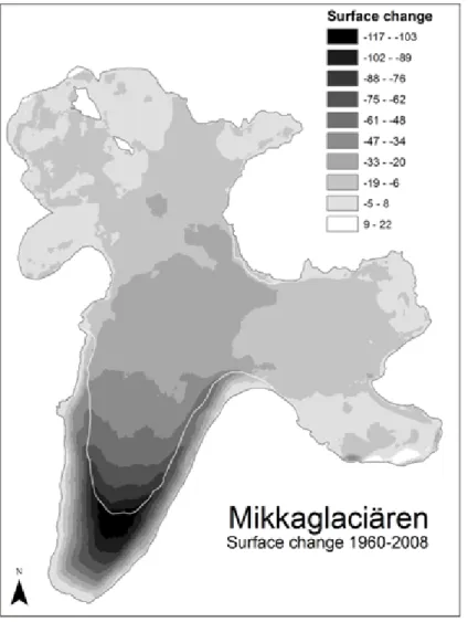
Figure Figure 2.2. Surface elevation change of Mikkaglaciären between 1960 and 2008, indicating dramatic thinning over the tongue, with more modest surface lowering in the accumulation zone.

Between 1895 and 1901 ice velocity surveys were conducted along

transverse profiles on the glacier tongue (Hamberg 1901 and 1910). In 1983 the tongue was radio echo sounded and a surface map constructed based on aerial photographs from 1980. These two datasets allowed for the calculation of balance ice flux, from which it was determine that in 1900 the glacier was close to its maximum, but was far from a balanced state, as the balance flux exceeded the surveyed ice flux by 3-4 times in the upper part of the glacier tongue (Holmlund 1986). The mass balance gradient needed to support this long, slowly moving ice tongue is on the order of 0.1 m w.e. /100 m, which is extremely low (Holmlund 1986). Balance flux calculations also showed that the position of the front was not in a stable state, and since the climate during the 19th century was cold and probably drier than the 20th century, this indicates either that there was a delicate balance between different climatic parameters to stop it at the position it stood at a century ago, or that the glacier underwent a surge and the old velocity surveys were carried out during a quiescent period.

(22)

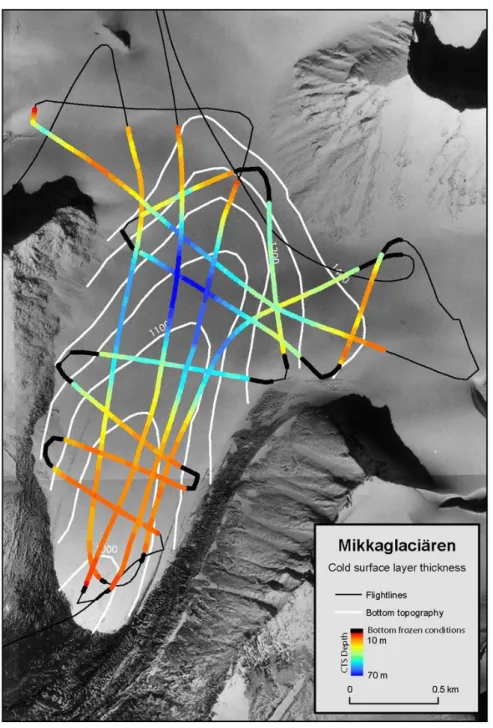
High frequency radar soundings of Mikkaglaciären indicate temperate conditions in the accumulation area and polythermal conditions in the lower part of the tongue, with a cold surface layer approximately 20 m thick. At the confluence of ice flowing from the two accumulation zones, the cold layer is extensive, with a thickness of approximately 70 m.

Figure 2.3. Thickness of the cold surface layer as surveyed along flight lines. Figure credit: R.Pettersson.

(23)

A hundred years ago the ELA of Mikkaglaciären was situated downstream of the confluence between the two accumulation areas. The ice at this confluence was most probably temperate, with the ice at the bed at the pressure melting point. When temperatures increased during the 20th century the ELA slowly migrated to a position upstream of the confluence, becoming an area containing superimposed ice, and later became an extension of the ablation area. The temperature of the ice at the confluence then cooled, and today it is characterized by cold ice throughout the ice column. This forms an obstacle for ice flow towards the front and acts like a dam to the ice upstream. The lack of ice flux towards the front may then explain the strong response to the recent relatively warm summers. If climate should change such that it promotes glacier growth, the glacier might grow thicker and the ice at the bed of the confluence area might become temperate, creating the prerequisites for a glacier surge (Clark et al. 1984, Murray et al 2000).

2.2.3.2. Storglaciären

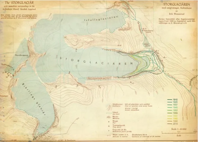
Storglaciären is by far the most studied glacier in Sweden, with a mass balance program, the longest in the world, having been initiated in 1945/46 (Schytt 1947). The glacier is located on the east side of the Kebnekaise massif and extends from 1750 to 1140 m a.s.l., covering an area of 3.1 km2, with a volume of 0.3 km3 (Bolin 2014, Holmlund 1993, Zempf et al. 2012). Photographic documentation of Storglaciären began in 1886, and the glacier front was surveyed for the first time in 1897 (Svenonius 1910). The thermal structure of Storglaciären was mapped for the first time in 1989 (Holmlund and Eriksson 1989) and a time series of thermal changes was analyzed by Pettersson et al (2007).Terrain models have been constructed based on aerial photos from 1959, 1969, 1980, 1990, 1999 and 2008 (Zempf et al 2012), and radar surveys have been conducted frequently since 1989.

(24)

Figure 2.4.The recession of Storglaciären between 1910 and 2012 (Holmlund 2012).

Both mass balance data and front position surveys indicate modest changes during the last three decades. In this sense the glacier is not really

representative of the general change in Swedish glaciers. The glacier was close to a steady state in the late 1980s (Holmlund 1988) followed by a period of growth which lasted until c.1996. This has since been followed by a gradual pattern of thinning, albeit somewhat less than that experienced by many other Scandinavian glaciers (WGMS 2012). The resurvey by

Pettersson et al. (2007) of the cold surface layer thickness indicated a general thinning of 10 m between 1989 and 2007 (0.55 m/year), with a change in average depth from 30 m to 20 m. Over that period the ice surface experienced negligible thinning, thus the study concluded that climatic warming had forced the change in cold surface layer depth between 1989 and 2007 (Pettersson et al. 2007).

2.2.3.3. Mårmaglaciären

Mårmaglaciären is located in the eastern Kebnekaise area, an area typified by a relatively dry climate. Mårmaglaciären is east facing, ranging between 1350 and 1740 m a.s.l., and is 3.8 km2 in area, with a volume of 0.4 km3 (Holmlund 1993, Bolin 2014). The first documentation of Mårmaglaciären are photographs taken in 1918, with more extensive photographic

documentation from 1952. The bottom topography was mapped by ground penetrating radar between 1984 and 1987, and the thermal structure in 1995 (Holmlund et al 1996). The glacier was included in the national front surveys

(25)

in 1968 and field surveys of its annual mass balance have been conducted since 1988. Digital terrain models exist from the years 1959, 1978, 1991 and 2008. Radar mappings were executed in 1995 and 2011-14. Between 1918 and 1959 the total frontal recession amounted to100 m, as the tongue was dammed by ice-cored moraines. When the thinning snout reached the flat bed floor the recession rate increased significantly and is presently about 15 m per year.

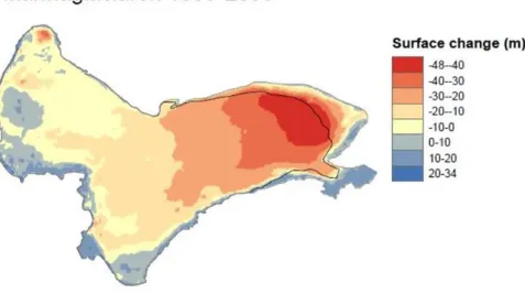
Figure 2.5.Thinning of Mårmaglaciären between 1959 and 2008. The 2014 front position is depicted in black.

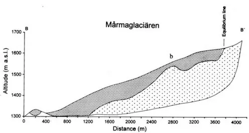
The cold surface layer was mapped along a series of radar profiles in 1995 (Holmlund et al. 1996), and between 2010 and 2014. The radar profiles from 1995 are too sparse to make any quantitative comparisons with the present state, but the longitudinal profiles indicate a general thinning trend. In the central part of the tongue the average depth was 74 m in 1995 and the corresponding depth in 2014 was 57 m, which implies a thinning rate of 0.9 m/year. However, as indicated in figure 2.6 there is a strong transverse gradient in the thickness of the cold surface layer on tongue and the 1995 survey was not positioned with GPS so it is difficult to make an in-depth spatial comparison between the present day and 1995.

(26)

Figure 2.6. The present cold surface layer on Mårmaglaciären as mapped in 2014.

Figure 2.7.The longitudinal profile of Mårmaglaciären from 1995. The grey dotted surface is cold ice and the white dotted area is temperate ice (Holmlund et al 1996).

2.2.3.4. Pårteglaciären

Pårteglaciären is located in the southeastern region of Sarek National Park. It extends from 1860 to 1100 m a.s.l., covering 10km2 with a volume of approximately 0.8 km3 (Bolin 2014, Holmlund 1993). The glacier was studied in the 1890s by Hamberg (1901), with mass balance information and photographic documentation existing from this time. In the 1960s it was included in the national glacier front monitoring program, and in 1997/99 a mass balance program was executed by Klingbjer (2001). The annual recession rate 1901-1963 was 4.7 m, and the corresponding rate for 1992-2013 is 15.9 m and 25.1 m for the last five years (Blomdahl 2015). The

(27)

thermal structure of the glacier was surveyed in 1996 and again between 2010 and 2014. Ice surface digital terrain models exist for the years 1963, 1992 and 2008.

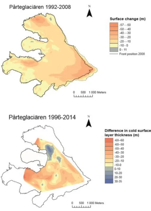
Figure 2.10 The average thinning of the cold surface layer between 1996 and 2014 and ice surface lowering between 1992 and 2008.

2.2.3.5. Kårsaglaciären

Kårsaglaciären (68°21´N, 18°49´E) is situated in the Abisko mountains and has an area of 0.85 km2 (Bolin 2014). It was first described scientifically by Svenonius in 1884, including surveys of ablation, ice velocities and front position (Svenonius 1910). Mass balance measurements have been carried

(28)

out occasionally since 1926, when the first detailed map was constructed. At this time the glacier area was 2.63 km2. The recession since then has been dramatic. In addition to the 1926 map, detailed maps have been constructed for the years 1943, 1959, 1970 and 1992. In 2013 Rippin et al (written communication) constructed a digital elevation model based on laser

scanning. They also mapped the thickness of the glacier and the thickness of the cold surface layer (Rippin et al. 2011). The structure of the cold surface layer on Kårsaglaciären is complex as the glacier ice is relatively thin after experiencing major thinning over the last century. The thinning is connected to climate change and explained by an increased winter air temperature since the mid-1980s (Pettersson et al., 2007). Sensitivity analyses indicate that an increase in surface temperature by 1°C would explain most of the observed change in the cold surface layer (Pettersson et al., 2007). An increased air temperature changes the upper boundary condition for the temperature distribution in the ice, which leads to a reduced freezing rate at the base of the cold surface layer.

The cold surface layer on Storglaciären is disappearing in the ablation zone and becoming more temperate, while Kårsaglaciären is losing the zone of temperate ice in the ablation area and consequently becoming colder. Thus there is clearly diversity in how the internal thermal structure of Swedish glaciers will change with a changing climate (Rippin et al., 2011).

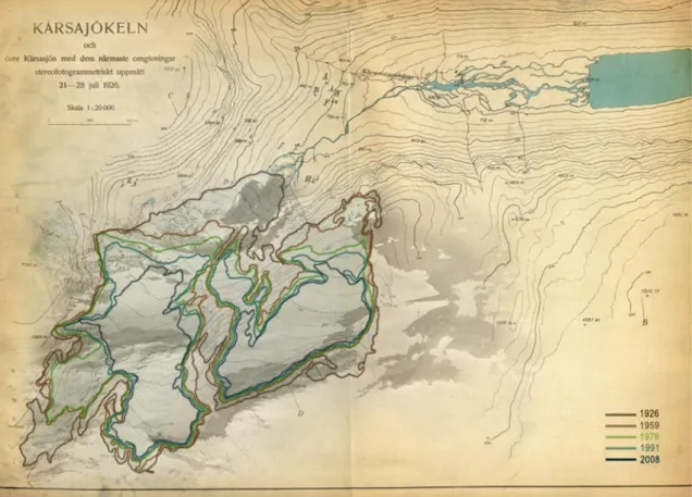
Figure 2.11. The dramatic recession of the Kårsaglaciären between 1926 and 2008. The south-eastern part of the glacier became decoupled from the main part of Kårsaglaciären in the 1950s, and is now a separate glacier named Östra Kårsaglaciären (Holmlund 2012).

(29)

2.2.4. Discussion

Rippin et al (2011) suggested that small glaciers are not able to adjust their temperature distribution if they are thinning rapidly. Thinning may thus lead to an average cooling of the ice body, as the cold surface layer remains while the temperate part is vanishing. Kårsaglaciären lost more than 50% of its mass between 1990 and 2008. Pettersson et al. (2007) showed that the change in thickness of the cold surface layer on Storglaciären was caused by climate during the same period, when the glacier lost less than 1% of its mass. These two studies are basically supporting each other, but the question raised herein is what happens during major geometry changes on large glaciers which are capable to match cooling with ice flux? In this study we have added another three glaciers with data on thermal distribution and glacier geometry and their changes over time. The thermal structure of Mårmaglaciären and Pårteglaciären were mapped 1995-96 and again 2013-14. Over this period they have lost a significant amount of ice mass and the cold surface layer has thinned on both glaciers. The spatial pattern of the thinning is evenly distributed over the glaciers, while the geometry changes show a strong correlation with the atmospheric temperature lapse rate causing large ice mass losses at low elevation and modest thinning at high elevation. Our interpretation of the observed temperature regime change is that it is rather caused by climate warming than by thermal/physical effects of the ice mass loss. We may also conclude that the thickness and spatial pattern of the cold surface layer responds sensitively to short term changes in climate. On Mikkaglaciären time series on the temperature distribution are lacking, but are existent on glacier geometry changes. The extent and thickness of the cold surface layer was mapped in 2010-12, but though older data are missing the pattern of the cold surface layer indicate a significant late thickening caused by a gradual increase of the ELA, transforming a gently sloping part of the accumulation area into an ablation area. This area with ice at below freezing point temperatures, act now as an obstacle for ice flux from the accumulation area to reach the snout which has led to a significant increase in recession rate. We have seen changes in thermal structure on all glaciers and the changes in cold surface layer caused by climate is on the order of -1 m a-1, similar in number but spatially different to the ice thinning over the time periods studied.

(30)

3. Spatial and temporal changes of ice

sheets

3.1. Background

The temperature distribution within a glacier or an ice sheet exerts a control on flow dynamics and hydrology. The ice temperature also affects the glacier hypsometry, interaction with the bed and the interaction between the glacier and groundwater (Cuffey and Paterson 2010).

In a maritime environment, such as the western part of Norway and the south coast of Iceland, the precipitation and ablation rates are high, giving high rates of mass turn over (WGMS 2008). The mass surplus of snow in the accumulation area is heated by refreezing melt-water every summer, forming temperate ice. In the ablation area the ice surface canbe cooled by low winter temperatures but this frozen top layer melts off each year in the summer, allowing the glacier to remain temperate. A temperate glacier is believed to be permeable to melt water. Water drains in a dendritic englacial system, with small veins close to the ice surface and successively larger conduits with depth as a consequence of an increased water-flow and thus increased melt rate (Shreve 1972). Estimations of the content of liquid water in a temperate glacier are often about 1-2%. The direction and inclination of the englacial water flow is governed by the ice surface slope. At the base of a glacier water flow is directed by the force of gravity plus the weight of the overlying ice (Cuffey and Paterson 2010). This simple model for water flow fits well with observations but it implies a system in equilibrium, with a hydrostatic pressure at the bottom equal to the overburden pressure. In practice it would mean that the influence of seasonal changes in meltwater flow is negligible. This is valid for the winter season but probably not during the melt season when the subglacial water pressure drops and has significant variability (Holmlund 1988b). However, studies of polythermal glaciers indicate that the seasonal changes has a minor effect on the general drainage pattern of the glacier (Fountain et al 2005, Holmlund 1988b)

The presence of water at the bed of a temperate glacier allows it to slide over its substratum, with the by-product of erosion. Diurnal and seasonal

variations in subglacial water pressure influence the geometry of the drainage system and the sliding speed significantly (e.g. Iken and

Bindschadler, 1986). Direct measurement of glacial erosion is difficult, and the most common estimations are based on silt load measurements in proglacial streams. Assuming a uniform erosion rate beneath a glacier and a steady state, silt loads may be transformed into erosion rates but with large degrees of freedom. However, such measurements include sediments derived from parts of the basin which are ice free. In particular, the area immediately in front of the glacier, from which ice may have retreated recently, will contribute with sediment from surface runoff in proglacial areas. This becomes a source of error in estimates of subglacial erosion rates, which is difficult to quantify (Holmlund et al. 1996). The erosion rate for

(31)

per year (Schneider and Bronge 1996). Thus, it is reasonable to assume an erosion rate of about 1 mm/year for glaciers in the Scandinavian mountain range.

In drier environments, precipitation and ablation rates are lower giving lower rates of mass turnover (Holmlund and Schneider 1997, WGMS 2008). It is common for the winter cooling depth to exceed the depth of summer melting causing a permanent sub-frozen top layer in the ablation area of the glacier (Holmlund and Eriksson 1989, Björnsson et al. 1996). Depending on winter temperature and summer melt rates, this cold layer can be more or less thick on such polythermal glaciers. In a dry polar climate the entire ice body may be at a temperature well below the freezing point, though melting occurs at the ice surface during the summer. These glaciers are referred to as subpolar. However, as melting occurs during the summer, it is common that temperate ice is produced at the higher reaches of the glacier while the entire ablation area is below the freezing point and frozen to its bed (Björnsson et al. 1996). A glacier which is entirely below freezing point temperature is herein assumed not to slide over its substratum with no liquid water present at the interface between bedrock and ice. Striae formation may still occur via mechanical erosion if basal ice is debris rich (Shreve 1984).

As ice below the freezing point is impermeable to meltwater there is no englacial drainage in cold glaciers except for surface drainage channels which can, if they carry large quantities of water, melt down into the ice and form conduits called cut-and-closure channels (Gulley et al., 2009). In the coldest environments, such as on top of the Greenland and Antarctic ice sheets, no melting occurs and thus the ice surface temperature remains equal to the local annual mean temperature. This is the high polar environment from which deep drilling projects have yielded comprehensive

environmental and climatic data. This is also the environment which best corresponds to glacial maxima of the Scandinavian Ice Sheet during the Weichselian. The temperature regime within such an ice sheet is a function of the air temperature at the surface, the vertical movement, advection of ice, heat conduction, internal friction and the geothermal gradient. If there was no ice movement we could simply extrapolate the geothermal gradient from the bed beneath through the ice (Cuffey and Paterson 2010), but this situation is unrealistic for most part of a glacier or an ice sheet. It is

unrealistic because the mass balance is positive on the centre of an ice sheet (to maintain the shape of the glacier), thus producing a vertical movement. The temperature regime governs not only the erosion capacity of a glacier but also the viscosity of the ice, which influences ice flow through deformation. Ice at the pressure melting point deforms ten times more quickly than ice at –20°C (Cuffey and Paterson 2010). Physical factors which influence basal temperatures are: precipitation rates, ice thickness, geothermal gradient, ice movement, and ablation rates. Dissipative heat production via internal friction becomes increasingly important with depth since deformation gets higher with depth due to increasing shear stress and frictional heating at the bed. On the Greenland ice sheet, ice is formed at the surface at temperatures 20-30 degrees below the freezing point. Where the ice is sufficiently thick it reaches the pressure melting point at its base due to the pressure exerted by the overlying ice. Towards the margins, ice will

(32)

freeze onto the bed as a result of thinner ice. In the case of ice streaming, the high rate of deformation and enhanced basal sliding via meltwater

lubrication produced fast velocities, warming the base far into the interior of the ice sheet, along the flow line of the ice stream.

3.2. Basal conditions in East Antarctica

In our search to understand glacial processes three different approaches are typically taken: mapping landforms from past glaciations; studying glacial processes on contemporary glaciers; and conducting modelling experiments. In Antarctica we have the opportunity to take a fourth approach; using geophysical techniques to study the subglacial landscape during an ongoing glaciation. The East Antarctic Ice Sheet can be viewed as an analogue for glacial maxima of the Scandinavian Ice Sheet. A range of basal conditions exist under Antarctica. Where ice is cold based, fragile landforms such as eskers may exist, preserved under the ice sheet, formed under a climate warmer than present conditions. In other areas of thick ice, basal conditions at pressure melting point allow for the formation of subglacial lakes, which recent studies have shown may have connectivity with other lakes (e.g. Wingham et al., 2006; Wolovick et al., 2013).

In western Dronning Maud Land there is considerable diversity in the glacial environment. Close to the coast there are glacially-eroded mountain ranges with large blue ice areas and supraglacial lakes (Holmlund and Näslund 1994). Some of these lakes have been observed to drain through the ice (Holmlund 1993, Jonsson 1988) in a manner similar to the frequent lakes drainages on the Greenland ice sheet. In between the mountain ranges there are deep tectonic troughs extending to 1000 m below sea level which contain ice streams that are currently operating (Fretwell et al 2013, Fujita et al 2009). Results of numerical ice sheet modelling suggest that the coastal area is very sensitive to sea level changes in a manner similar to West Antarctica (Näslund et. al 2000). A major increase in sea level may cause a collapse of the ice stream(s), with the mountain ranges becoming islands, which could have a dramatic effect on the pattern of ice flow and erosion. Further inland the majority of the land surface is above sea level and the ice sheet thus becomes robust (Fretwell et al 2013).

The concept of an Antarctic landscape formed under a past warm climate was first(described by Hans W:son Ahlmann (1944) when he took part of the photographic information sampled by the German Antarctic expedition in 1938/39 (Ritscher 1942). The relief of the landscape showed that the climate must have been different in the past and this fact linked to the question whether or not the present ice sheet was in a state of change as glaciers in the northern hemisphere did by shrinking as a consequence of climate warming (Ahlmann 1953). This idea became one of the arguments for the Norwegian-British-Swedish expedition in 1949-52 though the analysis of the landscape never was developed further.

In the pre site surveys of the European Deep Drilling Project EPICA large areas of Dronning Maud Land was mapped using radioecho technique for bottom topography and satellite positioning systems for surface mapping,

(33)

and numerical ice sheet models became available. Mappings of the

mountain ranges showed that the mountains no doubt were glacially eroded and modeling experiments suggested that this erosion may be very old, probably originating from the formation of the robust East Antarctic Ice Sheet some 17-35 millions of years ago a fact that opens new frontiers of scientific ideas to be developed (Holmlund and Näslund 1994, Näslund et al 2000).

In the early 1990s an increasing number of evidence confirmed the existence of a subglacial lake near the Vostok base. Old seismic data, new radio-echo data and analyses of the lowest lying ice in the deep ice core clearly

indicated the existence of a lake which later also was seen on satellite laser altimetry measurements. The existence of a subglacial lake beneath the Antarctic Ice Sheet was an eye opener and soon the number of potential lakes grew to over a hundred and the present figure is more than 400 lakes. However these lakes are of two fundamentally different kinds. The first one is large lakes such as the Vostok lake which has never been bottom frozen and includes organic life. There are only a few of this kind. The other type of lake is formed secondary when the ice sheet has grown thick enough to reach the pressure melting point at the base. These lakes may not have organic life, but play an important role in the subglacial hydrology and for the formation of landforms.

Within the international project BEDMAP data has been sampled by scientists worldwide to compile a bed topography map of Antarctica

(Fretwell et al. 2013). This compilation includes radar data from a variety of missions from pure mapping projects to detailed studies of small sites. A large number of sites have been sited where the bottom topography is flat and the reflection of radio-waves indicates liquid water at the base. These sites may not necessarily be proper lakes, but at least a wet surface.

However, the interpretations are often based on only little data. As a general rule of thumb there need to be at least 2500 metres of ice on top and the accumulation rate must be low to make the prerequisites for a subglacial lake to persist.

(34)

Figure 3.1. Basal conditions along the travelling route of the Japanese-Swedish Antarctic Expedition 2007/08 (Fujita et al. 2012). During this expedition three sites of potential subglacial lakes were investigated and supported earlier indications that they most probably are real lakes. The Amundsenisen site is marked Site 1 in both figures. The dashed line in the upper figure indicates at which depth the ice is believed to reach the pressure melting point. Data shows that along the profile different basal temperature conditions may exist. In the deeper parts these calculations are supported by radar signal processing. The colored surfaces within the ice body are isochrones from distinctive layers interpreted from radar signals.

(35)

At some sites such as in the western Dronning Maud Land there are flat basal surfaces seen on radar registrations on sites where basal melting is not expected. On a site at 75°S, 10°W a flat bottom was described by Näslund (1997). Calculations on ice temperatures indicate frozen bed conditions (Holmlund and Näslund 1994) and ice sheet models suggest a surface lowering during ice age conditions (Näslund et al. 2000). The hypothesis is that it is a sediment filled valley and not a lake.

Figure 3.2. The upper figure shows a radargram of a passage of site 1. A monopulse radar at 150 MHz was used from tracked vehicles and it was sampled January 17-19, 2008. The cartoon at the bottom shows what the landscape once may have looked like some 30 million years ago. The most interesting feature is the sediment filled valley shown to the left.

(36)

In western Dronning Maud Land mountain ranges act as efficient ice dams and the flow from the inland is concentrated into ice streams. The mountain ranges such as the Heimefront range reaches 2400 m a.s.l. and the ice surface elevation is approximately 2500 m on the proximal side and 1300 m on the distal side. Upstream this range there are other subglacial mountain massifs and ranges that are not visible on the surface. Radar soundings were performed during two days in January 1998 and January 2008 and a surface area of approximately 10x20 km2 was mapped. The ice surface elevation is 2500 m a.s.l. and the subglacial mountains reach up to 1600-1800 m. On an elevation around 500 m there is a 3 km broad valley with a flat bottom (Fig 3.2). Next to this valley there is a U-shaped fiord with a bottom at

approximately -500 m a.s.l. On the summits there are subglacial landforms very much like glacial cirques. If the flat bottom represents a sediment filled valley this landscape has remained more or less undisturbed since the ice sheet once was formed (Fig 3.2).

On the distal side of the Heimefrontfjella mountain range there is a large number of glacier cirques and subglacial indications of a former warmer climate. The Scharffenbergbottnen valley next to the Swedish station Svea was mapped during Swedarp 1987/88 (Holmlund and Herzfeld 1990) and the results highlighted two issues of importance. The valley is approximately 7 km long, 2 km wide and the ice thickness varies from about 300 m in the valley bottom to about 1000 m at the mouth. The valley is glacially over deepened (Figure 3.3). The ice surface is a blue ice area and the surface of the valley bottom is lying 150 m lower than the valley mouth. The present ice flux is directed into the valley as a result of high evaporation rates within the valley. The average annual temperature is -24 degrees. Though the ablation may cause a relative warming of the base there is no reason to believe that the over deepened basin relate to present erosion conditions but rather to something significantly older.

Figure 3.3. Bed topography of the Scharffenbergbottnen in the Heimefrontfjella range, East Antarctica (Herzfeld and Holmlund 1990).

(37)

4. Glacial geomorphology in the Gulf of

Bothnia, Åland Sea and

corresponding shores

4.1. Ice age scenario

Studying the morphology of the deglaciated landscape of Sweden gives an indication of the temperature regime of the former ice sheet. The interior of northern Sweden contains few signs of the effects of glacial erosion, whilst the coast of the Gulf of Bothnia and the Baltic has clear signs (Holmlund and Fastook 1993). In the Västerbotten area, on the north west side of the Gulf of Bothnia, there is a sharp line where drumlins change direction from south east in the inland parts to a more southern direction near the coast, indicating high ice velocities in the Gulf of Bothnia (Eklund 1988). In Tornedalen (north easternmost part of Sweden) the survived traces of fragile landforms indicate cold based conditions (Lagerbäck 1988). On the other hand, the closely located roche moutonées along the Swedish east coast are beautiful examples of both large and small scale glacial erosion. Thus from a glacial morphological viewpoint we may conclude that inland Sweden and, probably, also inland Finland were covered by cold based ice during the maximum phase of the Weichselian. During the phase of recession some areas may have experienced a change in thermal conditions from frozen base to thawed base as the frontal zone migrated backwards (Fastook and

Holmlund 1994).

The thermal conditions outlined here compare well with the present day ice sheet of Greenland, for which we can describe the boundary conditions fairly satisfactorily. Thus, the question is; what was the climate like during the last glaciation? Greenland ice cores indicate a climate during the later phase of the Weichselian at least 10-15 degrees colder than present (Johnsson et al. 1992). Assuming these figures are correct, and that the period lasted long enough for an ice sheet to form and to expand from the mountains in north-western Scandinavia towards the south, we will get a high polar ice sheet with a certain ice thickness and extent. Using an adiabatic lapse rate of 0.7-1.0 degrees Celsius per 100 m, we can assume annual temperatures around -40°C at the top center of the ice dome situated over the Gulf of Bothnia. If this estimation is reasonably correct we can conclude that the ice sheet over Scandinavia during the Weichselian was of a high polar type, similar to the present ice sheets over Greenland and Antarctica.

Based on temperature records interpreted from Greenland ice cores, the temperature during the first phase of the Weichselian glaciation may have been 4-5 degrees lower than at present (Johnsen et al. 1992). This likely led to significant increases in the extent of glaciers in the Scandinavian

mountain range, with the entire mountain range, except for high mountain peaks, likely ice-covered during the Early Weichselian (Fredin and Hättestrand 2001). At present the glaciers in northern Sweden are

polythermal (Holmlund et al 1996). In the event of air temperature cooling of a few degrees, the subpolar character of the glaciers would increase, but

(38)

the polythermal regime would persist, as the glaciers also would become thicker. Likewise, during the initiation of the Weichselian glaciation, it is probable that there was still temperate ice formation due to summer snow melt, despite the reduction in air temperature, especially in the high

mountain areas where localized net accumulation rates may have been large. Transferring our knowledge of individual glaciers to the entire mountain range during a period of predominantly westerly winds, we can infer that there would be more temperate glacial conditions on the west side of the range and more subpolar conditions on the east side (Holmlund and Schneider 1997). We may then expect that an early Weichselian Ice Sheet would have had more impact on the landscape through erosion on the western side of the mountain range and less impact on the eastern side. Superimposed on this east-westerly trend, there was also a vertical zonation, with areas characterized by basal melting in the deep valleys, and areas with ice below the freezing point at high altitudes. These scenarios are in

agreement with observations of preserved old weathering surfaces next to deep glacially excavated valleys.

On the eastern rim of the Scandinavian mountain range there are remnants of preserved ancient landscapes, indicating local frozen bed conditions

(Kleman 1992, 1994, Kleman and Borgström 1994). Thus, though glacial erosion was active in the central and western parts of the mountains, inland Sweden may have been characterized by permafrost and frozen interface between ice and bed.

The next phase of the last glaciation was when the ice sheet developed in size but was still smaller than during the glacial maximum. According to the Greenland ice cores, temperatures were only slightly warmer during this phase than during the last maximum phase (Dansgaard et al. 1993). Thus there is no reason to expect anything but a high polar ice sheet to form with frozen conditions under most of the ice sheet. Wet based conditions may have ocurred along the Norwegian west coast, in the Gulf of Bothnia, where large lakes are situated and perhaps some parts along the southern perimeter of the ice sheet.

The third and maximum phase is also characterized by a high polar ice sheet with well below freezing point temperatures throughout the ice body. Wet based conditions may have occurred in the deepest areas, which according to different data sets was centred in the Gulf of Bothnia. The length of the flow line through the Baltic turning west towards Denmark, indicates high flow rates, and the existence of an ice stream (Boulton et al. 1985, Holmlund and Fastook 1994, Torell 1878). This assumption is supported by the beautiful modified landscape which is slowly ascending by land uplift and by bathymetric data from the Gulf of Bothnia and the Baltic.

The temperature regime of the ice remnants during deglaciation was probably quite different than during the growing phase. Ablation rates were high, probably at same order of magnitude as thermal conduction speed in ice. During such conditions an ice body will preserve its thermal regime. A cold ice will remain cold during deglaciation.