Pricing commercial train path requests based on societal costs

Swedish National Road and Transport Research Institute

www.vti.se

Pricing Commercial Train Path Requests based on Societal

Costs

VTI Working Paper 2019:2

Abderrahman Ait Ali

_{, Jennifer Warg}

_{and Jonas Eliasson}

_{Transport Economics, VTI, Swedish National Road and Transport Research Institute}

_{Transport Planning, KTH, Royal Institute of Technology}

3

_{Communications and Transport Systems, Linköping University}

Abstract

On deregulated railway markets, efficient capacity allocation is important. We study the

case where commercial trains and publicly controlled traffic (“commuter trains”) use the

same railway infrastructure and hence compete for capacity. We develop a method that can

be used by an infrastructure manager trying to allocate capacity in a socially efficient way.

The method calculates the loss of social benefits incurred by changing the commuter train

timetable to accommodate a commercial train path request and based on this calculates a

reservation price for the train path request. If the commercial operator’s willingness-to-pay

for the train path exceeds the loss of social benefits, its request is approved. The calculation

of social benefits takes into account changes in commuter train passengers’ travel times,

waiting times, transfers and crowding, and changes in operating costs for the commuter

train operator(s). The method is implemented in a microscopic simulation program, which

makes it possible to test the robustness and feasibility of timetable alternatives.

We show that the method is possible to apply in practice by demonstrating it in a case study

from Stockholm, illustrating the magnitudes of the resulting commercial train path prices.

We conclude that marginal societal costs of railway capacity in Stockholm are considerably

higher than the current track access charges.

Keywords

Train timetables; societal costs; commuter trains; commercial trains; train path pricing.

JEL Codes

R40

1

Pricing Commercial Train Path Requests based on

Societal Costs

Abderrahman Ait Ali

_{, Jennifer Warg}

_{, Jonas Eliasson}

a _{Swedish National Road and Transport Research Institute (VTI)} P.O. Box 55685, 114 28 Stockholm, Sweden

1 _{E-mail: Abderrahman.ait.ali@vti.se, Phone: +46 (0) 8 555 367 81}

b _{KTH Royal Institute of Technology, Brinellvägen 23, SE-114 28 Stockholm, Sweden} c _{Linköping University, Luntgatan 2, SE-602 47 Norrköping, Sweden}

Abstract

On deregulated railway markets, efficient capacity allocation is important. We study the case where commercial trains and publicly controlled traffic (“commuter trains”) use the same railway infrastructure and hence compete for capacity. We develop a method that can be used by an infrastructure manager trying to allocate capacity in a socially efficient way. The method calculates the loss of social benefits incurred by changing the commuter train timetable to accommodate a commercial train path request and based on this calculates a reservation price for the train path request. If the commercial operator’s willingness-to-pay for the train path exceeds the loss of social benefits, its request is approved. The calculation of social benefits takes into account changes in commuter train passengers’ travel times, waiting times, transfers and crowding, and changes in operating costs for the commuter train operator(s). The method is implemented in a microscopic simulation program, which makes it possible to test the robustness and feasibility of timetable alternatives.

We show that the method is possible to apply in practice by demonstrating it in a case study from Stockholm, illustrating the magnitudes of the resulting commercial train path prices. We conclude that marginal societal costs of railway capacity in Stockholm are considerably higher than the current track access charges.

Keywords

Train timetables; Societal costs; Commuter trains; Commercial trains; Train path pricing

1 Introduction

The deregulation of railway markets in many countries have meant that it has become increasingly common that several operators run trains on the same track and hence compete for the same capacity. Inevitably, conflicts sometimes arise between different operators´ capacity requests, and in such cases the infrastructure manager needs to prioritise between conflicting path requests. Depending on the ownership of the railway infrastructure, the infrastructure manager can have different objectives; in this paper, we will consider the case where infrastructure is publicly owned, and the infrastructure manager wants to allocate capacity in a way that maximizes the total societal benefits.

There is a clear need for methodological development to overcome these challenges. Very large social and commercial values are at stake, so making the capacity allocation process more efficient can potentially generate substantial benefits. Moreover, the process and decision criteria need to be transparent and consistent to ensure fair and efficient competition between operators. In current practice, however, capacity allocation processes

2

are often opaque, and it is common that simplified decision criteria or rules of thumb are used, such as faster trains having priority over slower ones, or passenger services having priority over freight.

Highly simplified, there are two principal ways for an infrastructure manager to resolve conflicting path requests, either based on benefit judgments or on willingness-to-pay (WTP). In processes based on benefit judgments, the infrastructure manager compares some criteria or calculations intended to reflect the social benefits generated by alternative capacity allocations. The allocation which scores highest, according to these criteria, is chosen. In processes based on WTP, the operator that is willing to pay the highest price gets priority. Such processes include slot auctions and demand-differentiated track charges. Both methods have their respective strengths and weaknesses. The problem of the value-judgment is that data - crucial for judging the benefit of a service - is not always available. There exist well-developed methods to calculate societal benefits and costs of transport services, but such calculations are based on demand data, ticket prices and operating costs. For commercial traffic, such data is almost never available to the infrastructure manager, either because it is secret and sensitive business information known only to the operator, or because this data is unknown at the time of the decision. The problem in WTP-based processes is that the societal benefits of publicly controlled traffic – for example, the subsidized commuter trains serving many large urban regions – do not necessarily correspond with the responsible public agency’s willingness (or ability) to pay. Since the societal benefits of urban public transport cannot easily be “observed” in the same way as a commercial operator can observe its profits, it is much more difficult for public transport agencies to correctly assess its “willingness to pay” for capacity; both over- and underestimations may occur. Moreover, the societal benefits generated by urban public transport accrue to society at large, not to the agency, so there is no obvious link between the societal benefits generated by commuter train services and the responsible agency’s financial resources or hence its ability to pay for capacity. This is illustrated by the observation that public transport agencies are often under great financial strain, despite generating substantial societal benefits, not least because urban commuter trains are usually heavily subsidized (often for good reasons).

In this paper, we propose a hybrid method to resolve capacity conflicts between publicly controlled traffic (i.e. train services where supply and fares are determined by a public agency striving to maximize social welfare) and commercial traffic (i.e. train service run by a company striving to maximize profits, be it freight or passenger transport). For brevity, we will call the publicly controlled services commuter trains in the following. Such services are often run by one or more operators contracted by the agency, but this is inessential in this context.

The main idea of the proposed method is to calculate a reservation price for a commercial operator’s path request by estimating the societal cost (i.e. loss of benefits) of the changes needed in a baseline commuter train timetable to accommodate this path request. If the commercial operator is willing to pay this reservation price, it is awarded the path and the commuter train timetable is adjusted; if not, the request is declined. The process can be extended to handle multiple commercial path requests which also allows an infrastructure manager to prioritize between several commercial operators competing for the same capacity, i.e. on-rail competition.

This circumvents the problems explained above – on the one hand that an infrastructure manager does not have access to information necessary to assess the societal benefits of a

3

commercial train service, and on the other hand that there is no clear correspondence between public agencies’ WTP:s and the societal benefits generated by the services they run. Instead of only comparing benefit calculations or only comparing WTP:s, the process proposed in this paper compares benefit calculations for commuter train services to the WTP of commercial train services. The advantages of such a process is that it utilizes three key insights:

(i) The information needed for benefit calculations (fares, passenger volumes, operating costs etc.) for commuter trains is not secret and can be relatively obtained easily. (ii) Commercial operators have a relatively good perception of the profit they would

make on a given train path, and hence of the price they are willing to pay for a train path request to be accepted.

(iii) The prevalence of discriminatory pricing (i.e. yield management methods) in commercial railway markets means that the producer surplus (the profit) of a service is close to the total societal benefit of that service.

The purpose of the paper is to develop and explain the proposed method, and to apply it in a real-world application. In a case study from Stockholm, we calculate reservations prices for a commercial train service by adjusting a baseline commuter train timetable in three different ways: removing a commuter train service, shifting its departure time, and increasing its running time by letting it wait along the line while the commercial train passes by. The corresponding reservation prices are calculated for three different time periods, morning and afternoon peak hours and mid-day off-peak and compared to the current track charges (Trafikverket 2017). The adjustments are done in the microscopic simulation tool RailSys (Radtke and Bendfeldt 2001) to guaranty conflict-free timetable solutions. The results show the practical feasibility of the method and indicate a realistic range of reservation prices that commercial trains should pay if capacity should be reallocated from commuter trains to commercial trains. We conclude that the reservation prices that we find are considerably higher than current track charges.

The paper has the following structure: Section 2 gives a brief literature review of recent research on train timetable assessment. Section 3 describes the method for calculating the societal costs of changes in a baseline commuter train timetable. Section 4 presents the case studies, with input data and results. Section 5 concludes.

2 Previous related research

Measuring different characteristics of train timetables has been the subject of several research papers. A classic and widely studied question is how timetabling affects total capacity. This can be studied with a combination of analytical methods, simulation and optimization methods (Abril et al. 2008). For reproducing railway operations in the best way, dynamic, synchronous, microscopic, stochastic simulation tend to work best (Borndörfer et al. 2018). In addition to capacity effects, operational characteristics of timetables such as punctuality, stability and robustness have been extensively studied. For example, Delorme, Gandibleux, and Rodriguez (2009) focused on the stability aspect of the train timetables by developing a timetable stability module that is used to build an optimization model for railway operation planning.

4

There are also studies evaluating the performance of timetables from a passenger perspective, for example Kunimatsu, Hirai, and Tomii (2012), who use microsimulation of both passengers and trains in the railway network. Passenger behavioural aspects such as avoiding transfers and choosing best routes are also accounted for. The timetable is evaluated based on the disutility of passengers due to delays and crowding. This evaluation model is useful to capture detailed aspects of single line train timetables with a passenger perspective. The use of big data helps study even larger networks such as in the work by Jiang et al. (2016). Other studies have attempted to aggregate multiple passenger-related aspects of train timetables such as the sum of weighted waiting times, average of unit waiting time and maximum ratio of waiting time to travel time into a fuzzy analytic hierarchy process (Isaai et al. 2011).

In the demand modelling field, there is a large literature on valuation of timetable characteristics (waiting times, transfers, reliability and so on), and the demand effects of changes in such variables, e.g. Hensher (1997); Hensher and Ton (2002). It is still rare, however, that these results are used to evaluate the societal efficiency of timetables or capacity allocation. The method presented here is relatively novel in that respect, even if there are of course precursors. For example, Adler, Pels, and Nash (2010) study how competition between airlines and high-speed rail may affect service levels, and how this affects the benefits of high-speed rail investments. Eliasson and Börjesson (2014) also apply cost-benefit analysis on timetable construction, highlighting the impact of timetable assumptions on appraisal of railway investments. Brännlund et al. (1998) is also an example of capacity allocation with a clear economic objective; they present an algorithm that schedules a set of trains to obtain a profit-maximizing timetable without violating track capacity constraints.

3 Evaluation Model

The general idea of the method is to calculate the loss of benefits in commuter train traffic incurred when adjusting their timetable to accommodate an additional commercial train path. This loss of benefits, measured in monetary terms, yields the price that a commercial train operator requesting the path has to pay. If the operator is willing to pay the requested amount (the reservation price), the operator is awarded the requested path; otherwise the request is denied. This guarantees that the capacity conflict is resolved in a way that results in (local) potential Pareto efficiency.

The method starts with an initial situation, where commuter trains are run according to a baseline timetable, and a train path request from a commercial operator which conflicts with the baseline timetable. To accommodate the path request, changes to the commuter timetable are needed. The method calculates the value of the loss of societal benefits resulting from this modified commuter train timetable compared to the baseline timetable, and this loss of benefits (measured in monetary terms) constitutes the reservation price.

The loss of benefits Δ𝐵 consists of two parts: the change in consumer surplus Δ𝐶 and the change in producer surplus Δ𝑃. The change in consumer surplus reflects all changes affecting passengers, for example changes in waiting times, crowding, transfers and travel time. The change in producer surplus reflects all changes affecting the operator, for example changes in operations costs and revenues. It is quite possible that a change may result in, for example, a loss of consumer surplus but a gain in producer surplus. Cancelling a train service, for example, would normally produce a gain in producer surplus by decreasing the

5

costs of operations, but a loss of consumer surplus, since some passengers may experience increased waiting times and increased crowding in the remaining trains. Other types of societal benefits, e.g. changes in emissions and tax revenues, are ignored since they are negligibly small in this context.

3.1 Calculating the Change in Consumer Surplus

Let 𝑇 be the number of passengers arriving at time 𝑟 to station 𝑖 to travel to station j. The matrix 𝑇 is called the (dynamic or time-dependent) origin-destination (OD) matrix. Let 𝑐 be the generalized cost of travelling from station 𝑖 to station j starting at time r, and define it as the sum of the fare 𝑓 , waiting time(s) 𝑤 and the in-vehicle time 𝑡 , converting the time components into money by multiplying with the value of waiting time 𝛽 and the value of in-vehicle travel time 𝛼, see equation (1) . As explained further below, 𝛽 is a non-linear function of the waiting time, and 𝛼 depends non-linearly on the crowding level in the train. For simplicity, we do not distinguish between waiting at the first station and waiting at transfer stations in this study; introducing this distinction is conceptually straightforward.

𝑐 = 𝑓 + 𝛼𝑡 + 𝛽𝑤 (1)

A change in the baseline timetable will cause generalized travel costs to change, possibly inducing a change in passenger volumes as well. Let exponents 0 and 1 signify variables before and after the change, respectively. The change in consumer surplus1 _{is defined as in} equation (2).

Δ𝐶 = 𝑇 𝑐 − 𝑐 +1

2 𝑇 − 𝑇 𝑐 − 𝑐 (2)

In the following, we ignore the second term in this expression, effectively assuming that 𝑇 = 𝑇 . This simplifies the exposition and the following calculations, and the approximation error is small2 _{for moderate changes in the generalized travel cost.}

The timetable consists of a number of train services indexed by k. Given the timetable and the OD matrix, the number of passengers boarding and alighting train service 𝑘 at station 𝑖, called 𝐵 and 𝐴 , can be calculated (as explained in more detail further below). The number of passengers on train service 𝑘 between station 𝑖 and the subsequent station along the service line is 𝑁 = ∑ 𝐵 − 𝐴 , where the summation is taken over the stations served by service 𝑘. This allows us to rewrite the change in consumer surplus from equation (2) as the difference in the relevant part of the aggregate generalized cost, denoted by 𝐶, before and after the change, see equation (3).

1 _{This definition rests on some conventional assumptions such as negligible income} effects and a locally linear demand curve.

2 _{If the demand elasticity with respect to generalized cost is 𝜀, the relative error of a} relative change in generalized costs 𝑝 is ; for example, a 10% change of the generalized cost, assuming a demand elasticity of -0.5, gives a relative approximation error of = 2.5%. As we only consider small changes in the timetable, 𝑝 will stay moderate.

6

Δ𝐶 = 𝐶 − 𝐶 , 𝑤ℎ𝑒𝑟𝑒 𝐶 = 𝛼(𝑁 )𝑡 𝑁 + 𝛽 𝑤 𝑁

∈

(3) The notation 𝑖 ∈ 𝑘 means that the summation should be taken over stations served by train service 𝑘; 𝑡 denotes the travel time from station 𝑖 to the next station with train service 𝑘; 𝑤 denotes the average waiting time for train service 𝑘 at station 𝑖.

A number of things should be noted. First, we assume that the timetable change does not affect fares, so the fare terms in the generalized cost cancel out. Second, the value of in-vehicle time 𝛼 depends on the number of passengers in the train between each pair of stations – the more passengers in the train, the higher is the weight (i.e. the disutility) of in-vehicle travel time. A change in the timetable will typically change 𝑁 and hence 𝛼, since the crowding levels change. Third, the value of waiting time 𝛽 depends on 𝑖 and 𝑘. This is because the marginal valuation of waiting time is falling, since when waiting times (or rather, headways) are long, passengers can adjust their schedule to avoid waiting at the platform, see (Fosgerau 2009) for a theoretical analysis of this. This matters mainly for long headways, however; in our case study, headways are so short that this distinction does not matter much. Finally, and most importantly, expressing Δ𝐶 in this way simplifies the implementation substantially, since there is no need to calculate and represent the entire generalized cost matrix 𝑐 , or even have precise data on the full OD matrix 𝑇 . It is enough to have data on the number of passengers in each train on each link (𝑁 ) and the arrival times of passengers to their departure stations (which determines their waiting times 𝑤 ). This data is much easier to measure than the full OD matrix or generalized cost matrix; station arrival data is often directly available from entry measurements (e.g. smartcard gantries), and passenger loads can be measured either by on-board counts, automatic counting or weighing systems. Of course, if the OD matrix is available, passenger loads, and average waiting times are easily calculated with standard software, e.g. the microscopic simulation tool RailSys. The latter method simplifies the calculation of Δ𝐵. Further, using a simulation software also allows for introducing delays in the model.

3.2 Calculating the Change in Producer Surplus

The producer surplus is the difference between total fare revenues and operating costs. In the following, we assume that the timetable change does not affect fare revenues (although allowing for this is straightforward). This means that we only consider the change in operating costs. The total relevant operating cost can be separated into three parts: costs proportional to trains’ running distances (e.g. maintenance), costs proportional to trains’ running times (e.g. staff), and costs proportional to the number of wagons necessary to run the timetable (capital costs for vehicles). Hence, we can write the change in producer surplus Δ𝑃 as Δ𝑃 = 𝑃 − 𝑃 where 𝑃 is calculated as in equation (4).

𝑃 = 𝐾 𝑡

∈

+ 𝐾 𝑑

∈

+ 𝐾 𝑁 ∗ (1 + 𝐾 ) (4) The number of wagons 𝑁 necessary to run the timetable is estimated based on the total number of train services using a basic vehicle allocation model. The parameters 𝐾 , 𝐾 , 𝐾 and 𝐾 are calculated by analysing the transit authority’s

7

total operating costs by type (e.g. train staff, maintenance, capital costs etc.), allocating them to most relevant proxy for variable costs (distance, time or number of wagons) and dividing by the corresponding total (total distance, total time, total number of wagons).

3.3 Parameters

The parameters that are used in the benefit calculations in the case study are taken from various sources: partly from the research literature, partly from the Swedish cost-benefit guidelines (Trafikverket 2016), and partly from the calculation manual of the Stockholm Public Transport Agency (sll 2017).

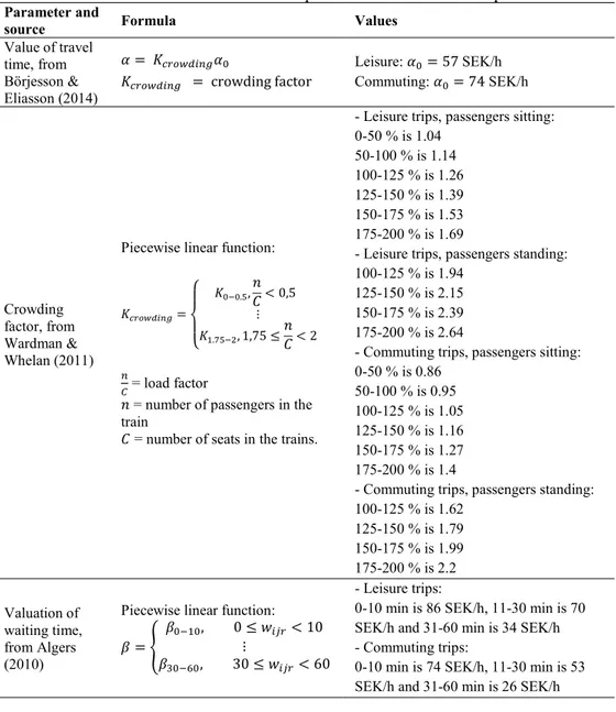
Table 1 - Parameters for the computation of the consumer surplus

Parameter and

source Formula Values

Value of travel time, from Börjesson & Eliasson (2014) 𝛼 = 𝐾 𝛼 𝐾 = crowding factor Leisure: 𝛼 = 57 SEK/h Commuting: 𝛼 = 74 SEK/h Crowding factor, from Wardman & Whelan (2011)

Piecewise linear function:

𝐾 = ⎩ ⎪ ⎨ ⎪ ⎧ 𝐾 ., 𝑛 𝐶< 0,5 ⋮ 𝐾. , 1,75 ≤ 𝑛 𝐶< 2 = load factor

𝑛 = number of passengers in the train

𝐶 = number of seats in the trains.

- Leisure trips, passengers sitting: 0-50 % is 1.04 50-100 % is 1.14 100-125 % is 1.26 125-150 % is 1.39 150-175 % is 1.53 175-200 % is 1.69

- Leisure trips, passengers standing: 100-125 % is 1.94

125-150 % is 2.15 150-175 % is 2.39 175-200 % is 2.64

- Commuting trips, passengers sitting: 0-50 % is 0.86 50-100 % is 0.95 100-125 % is 1.05 125-150 % is 1.16 150-175 % is 1.27 175-200 % is 1.4

- Commuting trips, passengers standing: 100-125 % is 1.62 125-150 % is 1.79 150-175 % is 1.99 175-200 % is 2.2 Valuation of waiting time, from Algers (2010)

Piecewise linear function: 𝛽 =

𝛽 , 0 ≤ 𝑤 < 10 ⋮

𝛽 , 30 ≤ 𝑤 < 60

- Leisure trips:

0-10 min is 86 SEK/h, 11-30 min is 70 SEK/h and 31-60 min is 34 SEK/h - Commuting trips:

0-10 min is 74 SEK/h, 11-30 min is 53 SEK/h and 31-60 min is 26 SEK/h

8

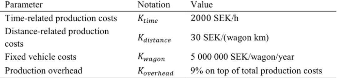
Table 2 - Parameters for the computation of the producer surplus (sll 2017)

Parameter Notation Value

Time-related production costs 𝐾 2000 SEK/h

Distance-related production

costs 𝐾 30 SEK/(wagon km)

Fixed vehicle costs 𝐾 5 000 000 SEK/wagon/year

Production overhead 𝐾 9% on top of total production costs

The notations, values and sources of the parameters that are used for the computation of the consumer surplus are provided in Table 1 whereas Table 2 provides the ones for the producer surplus (10 SEK is around 1€).

In the consumer surplus, we assume that the trip distribution is even between leisure and commuting trips, i.e. 50 % each (SL 2017). In the producer surplus, vehicle operation costs are estimated based on the total yearly travel distance and operation time for the trains and cost values according to the cost-benefit analysis recommendation from the local operator. Operating costs include capital costs and maintenance of the rolling stock, fuel and staff. Further, indirect costs including capital costs, overhead and administration are included based on the total number of passenger and rolling stock kilometres. The total costs are converted to daily costs by dividing yearly costs by the factor 320.

3.4 Estimation of passenger flow data

An important input to the calculation of the consumer surplus is the time-OD-matrix 𝑇 . We will briefly describe how it can be estimated from station entry data, and how it then can be used together with a given timetable to calculate passenger loads in the trains and waiting time costs. Handling trips with transfers is explained last, since this requires additional calculations.

Most public transport operators have access to data on the number of passengers entering each station during a certain interval of time, since this can usually be registered by most kind of entry gates. If some kind of smartcards are used, this becomes even easier. Let 𝑂 be the number of passengers entering station 𝑖 at time 𝑟. In our case study, we only have data on the total number of passengers during each 15-minute time period, so we assume that the arrival rate is constant over each such time period.

A common limitation (which is also the case in our case study) is that there is no station exit data, i.e. {𝐷 }, the number of passengers exiting station 𝑗 at time 𝑟, is unknown. To overcome this, we assume that trips are symmetric, meaning that the total number of passengers entering a station 𝑗 during a day is equal to the number of passengers alighting at that station: ∑ 𝑂 = ∑ 𝑇 . Together, this allows us to estimate the time-OD-matrix with a standard entropy maximization problem. See (Ait-Ali and Eliasson 2019) for more details.

In our formulas so far, we have tacitly assumed that the discretization of time, indexed by r, is sufficiently fine-grained compared to the discretization of the timetable. In a practical implementation, however, it is obviously inefficient to actually calculate and store the number of departures per station for each minute, or even second; instead, a constant rate of passenger departures per unit time is assumed to be known for each time interval, for example 15-minute periods. The number of passengers boarding a train is then easily calculated by multiplying the corresponding arrival rate(s) with the time elapsed since the

9

previous train departure. The number of passengers alighting a train can be calculated in a similar way.

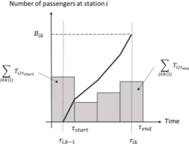
Let 𝑇 (𝑟) be the continuous rate of passengers entering station 𝑖 to travel to station 𝑗 at time 𝑟, and let 𝑟 be the departure time of train service 𝑘 from station 𝑖. The number of passengers boarding train 𝑘 at station 𝑖 𝐵 is then given by equation (5) where 𝑗 ∈ 𝑘(𝑖) denotes that the summation is taken over all stations 𝑗 served by train service 𝑘 from station 𝑖. 𝐵 = 𝑇 (𝑟) ∈ ( ) 𝑑𝑟 , (5) The time resolution of the rate 𝑇 (𝑟) depends on available data; in our case study, we have data on arrival rates per 15 minutes time period. Figure 1Fel! Hittar inte referenskälla. provides an illustration of the calculation of the number of boarding passengers 𝐵 . A similar method is used to calculate the numbers of alighting passengers 𝐴 .

Figure 1 – Calculation of the number of passengers 𝐵 boarding train 𝑘 at station 𝑖 using OD matrix 𝑇 .

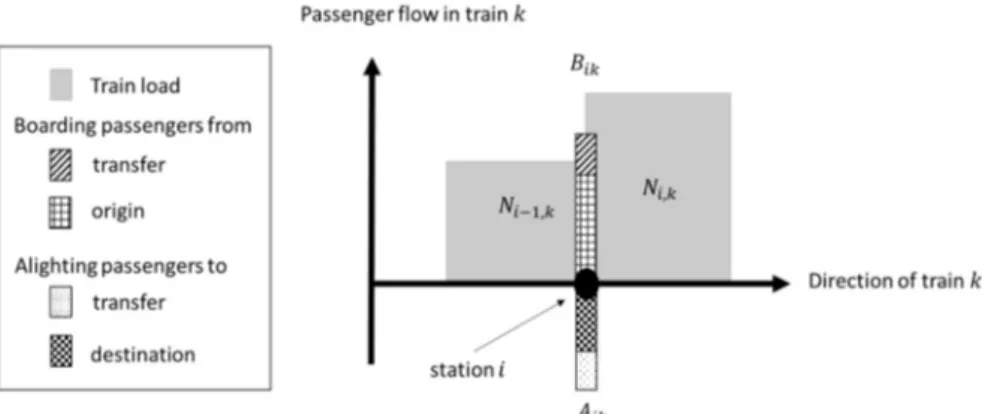
When dealing with passenger flows in complex train networks, it is necessary to handle trips that require transfers between train services. Given the OD matrix, transfer trips are split into two trips; one from the origin station to the transfer station and another one from the latter to the destination station. The number of passengers in each of the two trips is calculated using the same method as for any direct trip. These are added to the direct trips which gives the overall train loads including transfers. When there are several possible transfer stations, passengers are assumed to transfer at the first possible station. Figure 2 illustrates the passenger flow per link segment including transfer trips.

10

Figure 2- Passenger flow in train 𝑘 at station 𝑖 including transfers 3.5 Implementation

The network and the train timetables are modelled using the microscopic simulation tool Railsys which allows for instance to easily create, handle and simulate train timetables. There are many reasons for this choice, the main motives for the purpose of this paper are:

 Network, train and timetable models are provided in RailSys

 Manipulation and visualization of networks and train timetables is facilitated  Conflict detection (for timetable alternatives)

 Timetables simulation for the evaluation of feasibility and robustness  Data can be exported easily for integration with other software environments. The network is microscopically modelled in the simulation tool down to individual tracks, switches and signals. This gives more flexibility in investigating the effect of various aspects of the railway infrastructure on passengers and operators and the opportunity to check if a timetable solution is feasible. Due to the complexity of the network model, the network is always handled within the simulation tool and never exported outside.

The train timetables are however exported and used outside the simulation tool. This data is processed in order to extract information about arrival and departure times at every station, travel times and distances between stations. It is easy to create, modify and delete train paths for different train timetables scenarios. It is also possible to add potential delay distributions in the train timetable and simulate a certain number of days in order to estimate how the timetable will perform in operation.

4 Case Study

This section applies the method on a Stockholm case study, calculating reservation prices for a train path request during three different time periods (morning peak, mid-day, afternoon peak). The case study illustrates the practical feasibility of the method, and also

11

shows magnitudes of reservation prices, i.e. the loss of societal benefits in the commuter train system from allocating capacity to an additional commercial train

4.1 Description of the Stockholm commuter trains

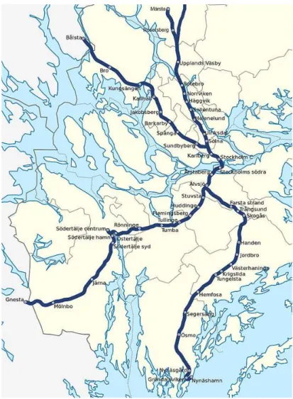
The Stockholm commuter trains (pendeltåg) share tracks with commercial passenger and freight trains. Figure 3 shows the network (in 2016). The network is mainly used by commuter trains, but the infrastructure in the northern parts, central Stockholm and some shorter sections is shared with commercial services such as freight, regional and long-distance passenger services.

12

The commuter network has an X-shape with around 50 stations along 240 km. All the trains pass a central section between Karlberg and Älvsjö. Commuter services are mainly operated in two channels, Södertälje-Märsta and Nynäshamn-Bålsta, complemented with additional services on shorter distances during peak hours. One of these complementary lines is prolonged to Uppsala via Sweden´s largest airport Arlanda. In addition, there is a branch connecting Södertälje to Gnesta (excluded in the case study for simplicity). Between Karlberg and Älvsjö, the major lines share the infrastructure. Stockholm central is the hub of the network allowing connections to services such as long-distance passenger trains, local and regional buses, airport shuttles and metro.

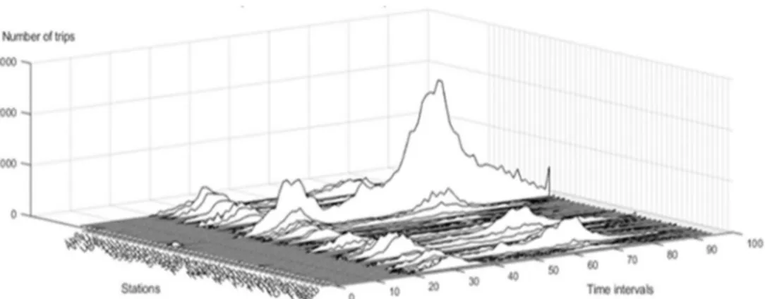
In 2016, the Stockholm region had 2.3 million inhabitants (SCB 2016). Figure 4 presents the number of departing passengers from each station across the day. There are major travelling peaks in the morning and afternoon and especially from and to Stockholm central.

Typical passenger loads for the different trains in a weekday in 2016 are presented in Figure 5. All trains running between Bålsta and Nynäshamn in both directions are included. The x-axis shows the links between two consecutive stations on the line, the passenger load is given on the y-axis. The horizontal dashed line represents the train (i.e. two wagon units) seat capacity. (In the case study, we assume that each train consists of two wagon units of the model Cordia X60 with a seating capacity of 374 passengers for each wagon unit (ALSTOM 2004)). Although there are extra train departures, crowding in the trains is common. The figure shows that passenger load on the line goes is well above the seat capacity for certain trains around the central station during peak hours.

Figure 4- Input data describing the trip distribution in origin station per time interval for one day (15 minutes over 24 hours) in the horizontal axis and the number of trips starting at the respective station in the vertical axis

13

Figure 5- Typical load of passengers of all the train paths during a weekday between Bålsta and Nynäshamn.

4.2 Allocating capacity for a commercial train path

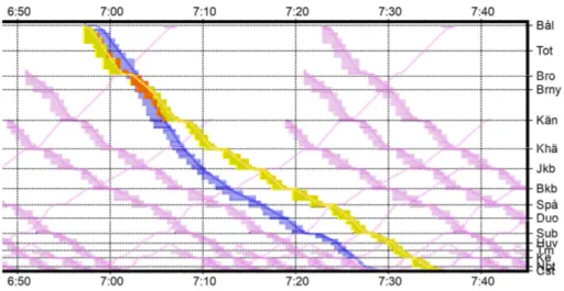
In this case study, a working day in September 2016 on the line Bålsta-Nynäshamn is used as baseline timetable. Figure 6 shows a graphical timetable, with a train path request in blue conflicting with a commuter train path in yellow. The conflict area is coloured red, and the commuter trains not involved in the conflict are coloured purple. In a graphical timetable, each line represents the scheduled time (horizontal axis) and location (vertical axis) in a train run surrounded by squares showing how long each train blocks the belonging signal sequence (block section). Each block section can only be used by one train at a time.

Figure 6- Graphical timetable showing a conflict (red) between a commuter train (yellow) and a commercial train (blue) during the morning peak (around 7:00 AM) on the line between Bålsta and Stockholm central station). Commuter trains not involved in the conflict are purple.

14

In order to resolve the conflict, the commuter train timetable can be changed in either of three ways:

(i) Scenario S1 – Remove: the conflicting commuter train service is cancelled. (Note that this means that the whole roundtrip train service needs to be cancelled.)

(ii) Scenario S2 – Delay: the commuter train´s dwell time at a certain stopping station is prolonged, in order to let the commercial train overtake.

(iii) Scenario S3 – Shift: the commuter train´s departure time at the first station is shifted, so that the commercial train can pass first.

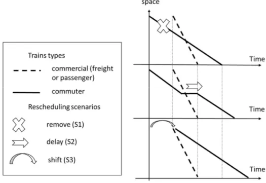
Changes were therefore made to the baseline timetable by rescheduling a certain train path using the different rescheduling scenarios, i.e. remove, shift and delay. These scenarios are illustrated in Figure 7 with the graphical timetable showing the conflicts between the subsidized and the commercial trains and the different rescheduling scenarios.

The last two scenarios (i.e. delay (S2) and shift (S3)) differ from a passenger point of view mainly in the way delays are experienced: Onboard in S2 (and for passengers boarding at a later station as waiting times at the platform), and at the station platforms in S3. That means the experienced delay is accounted for as an extra travel or waiting time.

Figure 7- Different experiment scenarios for conflicts between subsidized and commercial services

15

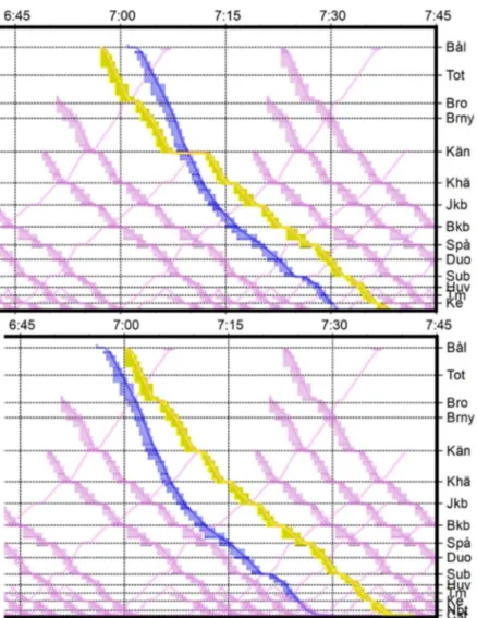
Figure 8- Illustration of two different commuter timetable changes for conflict solution: S2-delay (top) and S3-shift (bottom). Adjusted commuter train path in yellow, other commuter trains in purple, commercial train in blue.

These rescheduling scenarios, applied to the baseline timetable, are tested for conflicts in three different time periods, i.e. morning peak (6:00-9:00), noon off-peak (11:00-14:00) and afternoon peak (15:00-18:00). To illustrate this, Figure 8 shows two graphical timetables presenting two rescheduling scenarios, i.e. delay (left) and delay (right). The figure on the right shows the commuter timetable where the departure time of the conflicting commuter train path (yellow) has been shifted by +3 minutes whereas the one on the left shows that of delaying it in Kungsängen station for 4 minutes to let the commercial train pass. The third type of conflict solution (removing the conflicting commuter train path) is not presented in the figure.

16 4.3 Results

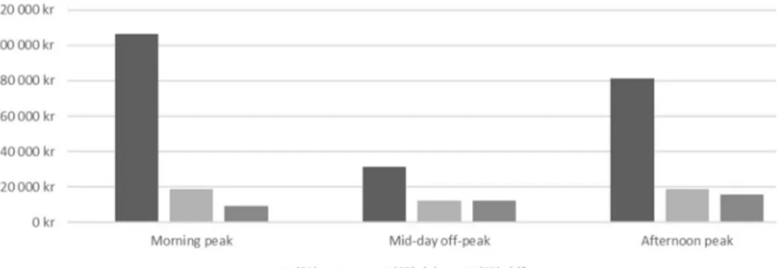
The total societal costs of the different rescheduling scenarios are presented in Figure 9. Changing the baseline timetable to accommodate the commercial train path can cause more than 100 kSEK (10 SEK is around 1€) total societal losses in the commuter train system, accruing to both passengers and operator(s). The minimal cost is incurred by shifting the departure time of the conflicting commuter train, resulting in a social loss of around 9-16 kSEK. Removing the conflicting commuter train path (i.e. scenario S1) always lead to the highest societal costs especially during peak hours. A less costly rescheduling strategy is to shift the departure time of the conflicting commuter train (i.e. scenario S3). Delaying the conflicting train at a certain station (S2) is also less costly but is more expensive than shifting the departures, especially in peak hours.

In order to give more details about the results in Figure 9, we present the different elements forming the total societal costs in Table 3 by showing the different passenger costs (i.e. travel time, waiting and transfer costs) and operator costs (i.e. distance and time dependent, fixed costs). The negative prices in Table 3 correspond to positive social benefits (cost savings), such as decreased operating costs or shorter transfer times. A dash means no difference in the costs relative to the baseline timetable.

Scheduling a commercial train leads to higher societal costs in the peak hours especially in the morning. This can be explained by the variation in the trip distribution, i.e. OD matrix, during the day, see Figure 4. Removing or cancelling the conflicting train always causes larger social losses than rescheduling the commuter train. Indeed, cancelling the conflicting commuter train leads to higher consumer costs compared to the gains in producer costs, which in turns lead to a high total cost especially in peak hours. However, delaying the departure of the conflicting commuter train in a stopping station leads to lower costs in both consumer and producer costs. The latter is due to the increase in operation time. Shifting the departure times of the conflicting commuter train causes no producer costs and generally lower consumer costs making this strategy generally better in this case.

Figure 9- Total societal costs of the changes to the baseline commuter train timetable in SEK.

17

Table 3 – Components of the total societal costs of changes relative to the baseline timetable (in SEK)

Scenario S1

Remove Scenario S2 Delay Scenario S3 Shift Total societal costs

(*) 104 955 (**) 30 554 (***) 80 761 16 242 10 661 19 203 9 247 10 630 16 044 Travel time 97 499 32 433 70 817 14 059 9 756 12 138 7 894 9 571 15 070 Waiting time 18 835 9 482 21 298 2 038 760 6 920 1 353 1 059 974 Transfer -476 -457 -451 - - - - - - Consumer (total) 115 859 41 458 91 664 16 096 10 516 19 058 9 247 10 630 16 044 Distance -6 370 -6 370 -6 370 - - - - - - Time -3 633 -3 633 -3 633 133 133 133 - - - Fixed -900 -900 -900 12 12 12 - - - Producer (total) -10 904 -10 904 -10 904 145 145 145 - - - (*) is for morning, (**) for mid-day and (***) for afternoon. This is for all the cells!

Based on these societal costs, one can compute the minimum cost that the commercial operator(s) should pay (to a certain infrastructure manager) so that it compensates the resulting losses in societal benefits. The first raw of Table 3, i.e. total societal costs, shows this minimal price for the different rescheduling scenarios and time periods of the day.

Compared to the current track charge for the train path, these total societal costs are substantially higher. Swedish track charges are made up of several components, one of which is set to partly reflect congestion (lack of capacity) on the tracks. For a train passing Stockholm, this “congestion charge” is 433 SEK (Trafikverket 2017), i.e. less than 5% of the minimal social loss caused by accommodating an additional train path. For instance, the

18

total track charge for a commercial passenger train Västerås - Stockholm C (sharing the track with the subsidised trains between Bålsta and Stockholm (45 km of the 105 km in total) is 1 454.46 SEK including power. Since the tracks are fully used for most parts of the day, the calculated costs can also be interpreted as the marginal value of increased capacity. It is possible that certain adjustments of the commuter train timetable may lead to positive social benefits rather than losses, since there is no absolute guarantee that the baseline commuter train timetable is strictly optimal. In such cases, the reservation price of the accommodated train path is of course zero (except for the usual charges for wear-and-tear etc.). In some cases, however, such results may be a sign that the parameters of the benefit-cost calculation, or its input data, may need to be adjusted. But non-optimal timetables may also sometimes be due to political considerations; there is anecdotal evidence of over-supply from other commuting train systems. Exploring the optimality of timetables from a benefit-cost perspective is an interesting research area of its own but is left for future research.

5 Conclusions and Future Work

This paper describes an approach to resolve conflicting capacity requests between commercial trains and public controlled traffic (“commuter trains”), by comparing the calculated loss of social benefits caused by accommodating the commercial train path and using this to price the train path. The calculation of benefits takes into account in-vehicle times, waiting times, transfers, crowding and operating costs.

The case study of the commuter train services in the Stockholm region shows that the evaluation model can be used in different situations to help planners evaluate the impact of their timetable choices. Results also provide insights into how the model can be used to price commercial train slots in conflict with the commuter train services. The results show that accommodating additional train paths in the busy commuter train timetable comes at a high societal cost – much higher than the current track charge intended to party reflect scarce capacity in Stockholm. We also show that it is possible to substantially reduce the costs of changes in commuter train timetables by choosing the right rescheduling alternative. This best alternative might not be evident to the planners without the help of a cost assessment model as the one presented in this paper.

The evaluation model that is presented in this paper is not limited to the experiment in the case study. It can be used in a number of other real-world situations to help railway planners make efficient changes to the timetables with minimal societal costs. Ideas for possible applications include the assessment of the societal effects of using a train timetable with skip-stops instead of all-stops. It is also possible to link the model to an optimisation model in order to find optimal train timetables given a certain trip distribution.

Additionally, one may also improve the model by including extra costs and accounting for negative and positive externalities. Many possible future works can help improve the quality of the assessment model and the case study that is presented in this paper. As mentioned in the limitations, the OD-data was incomplete, hence only an estimate was used. Applying the model in a case study with complete input data may provide more accurate results and insights. Moreover, socio-economic data on the passengers, if available, can be used with an improved version of the model where disaggregated results can be computed. In this way, one can get insights as to which (how much each) socio-economic group is winning or losing. This gives further insights on the equity of the train service operations.

19

References

Abril, M., F. Barber, L. Ingolotti, M. A. Salido, P. Tormos, and A. Lova. 2008. 'An assessment of railway capacity', Transportation Research Part E-Logistics and Transportation Review, 44: 774-806.

Adler, Nicole, Eric Pels, and Chris Nash. 2010. 'High-speed rail and air transport competition: Game engineering as tool for cost-benefit analysis', Transportation Research Part B: Methodological, 44: 812-33.

Ait-Ali, Abderrahman, and Jonas Eliasson. 2019. "Dynamic Origin-Destination-Matrix Estimation Using Smart card Data: An entropy maximization approach." In. Algers, S., Börjesson, M., Sundbergh, P., Byström, C., & Almström, P. 2010. "Valuation

of Time in Transport – The National Studies 2007/08 in Sweden." In Trafikverket rapport No. 2010:11, edited by Trafikverket.

ALSTOM. 2004. "CORDIA 60X." In.

Borndörfer, Ralf, Torsten Klug, Leonardo Lamorgese, Carlo Mannino, Markus Reuther, and Thomas Schlechte. 2018. Handbook of Optimization in the Railway Industry (Springer International Publishing).

Brännlund, U., P. O. Lindberg, A. Nõu, and J.-E Nilsson. 1998. 'Railway Timetabling using Lagrangian Relaxation', Transportation Science, 32: 358-69.

Delorme, X., X. Gandibleux, and J. Rodriguez. 2009. 'Stability evaluation of a railway timetable at station level', European Journal of Operational Research, 195: 780-90.

Eliasson, Jonas, and Maria Börjesson. 2014. 'On timetable assumptions in railway investment appraisal', Transport Policy, 36: 118-26.

Fosgerau, Mogens. 2009. 'The value of headway for a scheduled service'. Frohne, Erik. 2014. "Stockholm commuter train system map." In.

Hensher, David A. 1997. 'A practical approach to identifying the market potential for high speed rail: A case study in the Sydney-Canberra corridor', Transportation Research Part A: Policy and Practice, 31: 431-46.

Hensher, David A., and Tu Ton. 2002. 'TRESIS: A transportation, land use and environmental strategy impact simulator for urban areas', Transportation, 29: 439-57.

Isaai, Mohammad T., Aram Kanani, Mahshid Tootoonchi, and Hamid R. Afzali. 2011. 'Intelligent timetable evaluation using fuzzy AHP', Expert Systems with Applications, 38: 3718-23.

Jiang, Zhibin, Ching-Hsien Hsu, Daqiang Zhang, and Xiaolei Zou. 2016. 'Evaluating rail transit timetable using big passengers' data', Journal of Computer and System Sciences, 82: 144-55.

Kunimatsu, Taketoshi, Chikara Hirai, and Norio Tomii. 2012. 'Train timetable evaluation from the viewpoint of passengers by microsimulation of train operation and passenger flow', Electrical Engineering in Japan, 181: 51-62.

Radtke, Alfons, and Jan-Philipp Bendfeldt. 2001. "Handling of railway operation problems with RailSys." In Proceedings of the 5th world congress on rail research. Cologne: World congress on rail research.

SCB. 2016. "Population in the country, counties and municipalities on 31 December 2016 and Population Change in 2016." In.: Statistics Sweden.

sll. 2017. "Dokumentation av SAMS 3.0." In. Stockholm.