Calving Events Detection and Quantification from Time-lapse Images: A Case Study of Tunabreen Glacier, Svalbard

(1)

IT 15 038

Examensarbete 30 hp

August 2015

Calving Events Detection and

Quantification from Time-lapse

Images

A Case Study of Tunabreen Glacier, Svalbard

Sigit Adinugroho

(2)

(3)

Teknisk- naturvetenskaplig fakultet UTH-enheten Besöksadress: Ångströmlaboratoriet Lägerhyddsvägen 1 Hus 4, Plan 0 Postadress: Box 536 751 21 Uppsala Telefon: 018 – 471 30 03 Telefax: 018 – 471 30 00 Hemsida: http://www.teknat.uu.se/student

Abstract

Calving Events Detection and Quantification from

Time-lapse Images : A Case Study of Tunabreen

Glacier, Svalbard

Sigit Adinugroho

A fully automated method for detecting and measuring calving regions of a glacier is an important tool to gather massive statistical data of calving events. A new

framework to achieve the goals is presented in this thesis. First, time-lapse images are registered to the first image in the set. Registration process makes use of the

M-Estimator Sample Consensus (MSAC) method to estimate a transformation model that relates a pair of Speeded-Up Robust Features (SURF). Then, the terminus of a glacier is separated from other objects by a semi-automatic Chan-vese level-set segmentation. After that, calving regions in a terminus are detected as a combined difference of Local Binary Patterns (LBP) of two successive images. Clustered points that form a difference image are transformed into polygons representing changed regions by applying the alpha-shape method. Finally, the areas of changed regions are estimated by the pixel scaling method. The results highlight the performance of the method under normal conditions and reveal the impact of various weather conditions to the performance of the method.

Examinator: Justin Pearson Ämnesgranskare: Robin Strand Handledare: Dorothée Vallot

(4)

(5)

3 Description of the proposed approach 20 3.1 Data collection . . . 20 3.2 Implemented methods . . . 21 3.2.1 Registration . . . 22 3.2.2 Cropping . . . 22 3.2.3 Segmentation . . . 23 3.2.4 Change detection . . . 24 3.3 Evaluation strategy . . . 26 4 Results 28 4.1 Results under normal conditions . . . 28

4.2 Results under noisy environment . . . 32

4.2.1 Results under minimum illumination . . . 32

4.2.2 Results under low illumination change . . . 33

4.2.3 Results under high illumination change . . . 34

4.2.4 Results in the presence of fog . . . 35

(6)

5 Discussion 40 5.1 Performance and errors . . . 40 5.2 Evaluation technique . . . 41

6 Conclusions 42

6.1 Future work . . . 42

Appendices 48

(7)

List of Figures

1 Geographical location of Tunabreen glacier and the placement

of time-lapse cameras. . . 2

2 Illustration on how actual size of a pixel is estimated from an image pixel size. . . 5

3 Illustration of H matrix . . . 5

4 All possible locations of a contour relative to the object and their corresponding fittings . . . 12

5 Thresholded value and weight from a 3x3 grid . . . 14

6 Neighborhood map with various P and R. . . 14

7 α-hull and its corresponding α-shape from a set of points S . 16 8 Three polygons reconstructed from the same set of points. . . 17

9 A confusion matrix, comparing human judgment and an au-tomatic classification result. . . 18

10 An example of a binary change mask, as a result from a change detection method. . . 19

11 A sample image from the data set . . . 21

12 The flowchart visualizing overall framework . . . 22

13 Cropped version of Figure 11 focusing on the terminus . . . . 23

14 An example of the result of a segmentation process. . . 24

15 Detected changes from two consecutive images using standard deviation as the threshold. . . 24

16 Detected changes from two consecutive images using local threshold. . . 25

17 Detected changes from two consecutive LBP texture images . 25 18 Reconstructed change masks from two consecutive images . . 26

19 Change mask of normal1 sample images . . . 28

20 Change mask of normal2 sample images . . . 28

21 Change mask of normal3 sample images. . . 29

22 Change mask of normal4 sample images. . . 29

23 Distribution of Kappa coeﬃcient under normal conditions. . . 30

24 Distribution of missed alarms under normal conditions. . . . 30

25 Distribution of the most frequent missed alarms under normal conditions. . . 31

26 Distribution of false alarms coeﬃcient under normal conditions. 31 27 Distribution of the most frequent false alarms under normal conditions. . . 32

28 Change masks of images captured at midnight . . . 33

29 Some examples of results under low illumination. . . 34

30 Two images with high illumination change and their corre-sponding change mask. . . 35

31 Two possible state of noise in a change mask of two images with thin or medium fog. . . 36

(8)

32 An example of image covered by a thick fog . . . 36 33 Two change masks of images covered by thick fog. . . 37 34 Distribution of Kappa coeﬃcient for the entire data set. . . . 38 35 Distribution of missed alarms for the entire data set. . . 38 36 Distribution of the most frequent missed alarms for the entire

data set. . . 39 37 Distribution of false alarms for the entire data set. . . 39 38 Distribution of the most frequent false alarms for the entire

(9)

1 Introduction

1.1 Background

The rising sea level is predicted to have noticeable economic, social and environmental consequences. While the factors leading to sea level rise are known, an actual and precise prediction of it is diﬃcult to make. After thermal expansion, the most important contributor is the release of water from land ice (glaciers, ice sheets) as shown in the last IPCC report [1]. Unfortunately, ice flows non-linearly and processes at stake are not fully understood. Some glaciers, and most of those situated on ice sheets, are flowing directly into the ocean. These so-called calving glaciers are directly releasing blocks of ice - icebergs - into the ocean. The mechanism leading to calving is not understood even though its contribution to sea level rise is important. Some models have been proposed but none of them is accurate enough to perform good predictions.

A deeper understanding of calving activity and its related causing fac-tors requires large statistical data from long-term monitoring, especially on frequency and magnitude. An old fashioned but still widely used method of manual observation for gathering calving occurrence is prone to be inefficient and requires a long period of human work, where a group of observers build a camp to monitor the glacier for a certain time period. A semi-automatic method uses a camera to capture the face of a glacier and then iceberg dis-placement is located manually from a sequence of captured images. Later, the actual size and volume of a calving event can be derived from the pixel size of the images with the help of reference data from a satellite. Although the latter approach is significantly simpler than the former one, selecting a break-off location from hundreds of images tends to consume a lot of time and effort. In order to have a system with less human intervention, the calv-ing event detection from a sequence of images must be done automatically.

1.2 Goal

This project is intended to recognize calving events in terms of frequency and magnitude on Tunabreen glacier in Svalbard. Events are detected by analyzing changes on a sequence of pictures of calving terminus (the front face of a glacier) acquired by single time-lapse camera installed in front of the glacier and then quantified by approximating the size of individual pixel. The result of this work will be used to verify a recently developed particle model that reproduces calving glacier front.

1.3 Scope

The main focus of this research is to detect calving events from a set of continuous images under normal conditions. Normal conditions are defined

(10)

as clear weather conditions, ocean free from ice melange and images are cap-tured without over-exposure and artifacts. Observation has been performed on Tunabreen glacier located in Svalbard, Norway and a subset of images taken from 2-6 September 2014 is used as the data set. Generalizations to other glaciers and conditions are not required.

Figure 1: Geographical location of Tunabreen glacier and the placement of time-lapse cameras1. This project uses images captured by the camera installed in 2014.

(11)

2 Theory

This section focuses on theories implemented in this project. Since the project is a collaborative work, theories from both Computer Science and Geology fields are explained to help readers understand the concept of the work.

2.1 Calving as a cause of sea-level rise

Worldwide sea level always shows a rising trend. An early observation in the late 19th century revealed that sea level has arisen for around 1.7 _± 0.3 mm/year [2] and almost doubled in the period between 1993 and 2009 with mean value of 3.3 ± 0.4 mm/year [3]. The Intergovernmental Panel on Climate Change (IPCC) forecasted that global sea level will arise further from 0.18 to 0.59 m relative to the 1980-1999 situation by the end of the 21st century [1].

The physical and socioeconomic effects of sea-level rise (SLR) are well studied. SLR increases the occurrence and magnitude of several natural phenomenons related to disasters such as floods, storm, tsunamis, and ex-treme waves [4]. From an economic standpoint, it is assumed that SLR has four damage cost components : the value of dry-land lost, the value of wetland lost, protection cost for defending a location from SLR, and the cost for moving people from an SLR affected area to a safer place [5]. The negative effects of SLR pose serious impact on human life since 17 out of 30 world’s largest cities lie on coastal regions, including Mumbai (India), Shanghai (China), Jakarta (Indonesia), Bangkok (Thailand), London (UK), and New York (US) [6].

SLR is predominantly caused by two factors, expansion of water in oceans due to temperature increase and water transfer between ocean and other water reserves such as glaciers and ice sheets. The last IPCC re-port shows that sea level rises for average 3.1_{± 0.7 mm/year from 1993 to} 2003. Under the same period, it is estimated that thermal expansion con-tributes 1.6± 0.5 mm/year while water transfer from ice reservoir accounts for around 1.19 mm/year [1]. Water is released into the ocean through melting and direct displacement of blocks of ice into the ocean known as calving [7]. Under normal circumstance, mass lost from a tidewater calving is dominated by calving rather than surface melting [8].

Calving process of ice mass contributes significantly to the rise of global sea level. In spite of its critical impact, calving still hides unanswered ques-tion which is remarkable for its relaques-tion to external factors that control its occurrence. Current status explains that generic physical model for calving problem does not exist. So far, researchers only managed to reveal relation-ship between calving and external factors in specific regions. The reason why a calving model is hard to build lies in its multivariate nature and

(12)

variability over time and space [9]. The diﬃculties on making quantitative observation over calving event creates another gap for understanding the cause of calving process [8].

2.2 Calving observation techniques

The diﬃculties and risks in monitoring calving rate are some contributing factors to poor understanding of calving dynamics. Several attempts have been made to monitor calving activity, starting from a manual observation by building a camp nearby a glacier terminus and observing the calving frequency and magnitude visually. For instance, the observation conducted by O’nell et al. in 2005 at the terminus of Columbia glacier, Bartholomeus et al. in June 2010 at the Yahtse Glacier, and Youth Expedition program in July 2010 at the Sveabreen glacier [10].

2.2.1 Photogrammetry technique for calving observation

Photogrammetry technique, which uses a time-lapse camera at a distance from the front of a glacier, provides more sophisticated way to measure calving activity by omitting the need of human observer. Compared to a remote sensing using airborne or satellite sensor, camera-based observation is able to achieve higher precision. A common pixel size of remote sensing images range is 10-30 m with eﬀective precision in kilometers, while the eﬀective precision of a photogrammetry observation is measured in meters [11].

Opposed to a satellite image that is relatively free from noise, image cap-tured by a camera is influenced by surrounding natural phenomenon that may generate a noise. Ahn and Box expound common problem in camera-based glacier observation [12]. Snow, rain, and fog lessen the clarity of captured images. Extreme illumination condition, both overexposure and underexposure, may not be handled by camera auto exposure eﬀectively, dropping the detail of the image. Furthermore, wind does not introduce noise but slightly changes the position of a camera, thus creating misaligned images. The misalignment can be normalized using a technique called im-age registration. Huang et al. [13] and Radke et al. [14] also emphasize the importance of registration process as a preprocessing step in a change detection process.

2.2.2 Estimating area of calving regions

The area of a calving region is estimated by taking advantage of the pixel scaling method [15]. The actual size of a pixel in a camera’s sensor can be estimated using the Thales Theorem as illustrated in Figure 2. If the pixel size x, the focal length f of the lens, and the distance h from the camera to the point in the terminus which corresponds to a pixel in the sensor are

(13)

known, then the actual size X of the pixel is estimated by the following formula : h f = X x· (1)

Figure 2: Illustration on how actual size of a pixel is estimated from an image pixel size.

The real area of a pixel is estimated as X2 _{and the real area of a calving}

region is computed as the sum of real area of all pixels which constitute the region.

The pixel size of the camera’s sensor and the focal length are known as parts of camera properties (see Table 1). Distances of the camera to points in the glacier front are determined by referencing to a satelite imagery. Then, they are tabulated in the matrix H as shown in Figure 3. A cell hi in the

matrix represents the distance of the camera to the location in the terminus which matches a pixel in the sensor. It is assumed that there is no vertical distortion, thus every point at the same column has an equal distance to the camera.

(14)

H

f =

X

x· (2)

2.3 Automated feature extraction and image registration

Image registration is a process of superimposing two images of the same object captured at different time, from different angle, or by different sensor through aligning shared features in both images. Registration is a key suc-cess for image analysis work where images are taken from different sources or time, like in a change detection process. In general, a feature-based image registration consists of four steps : feature detection and extraction, feature matching, transform model estimation, and image transformation and image resampling [16].

2.3.1 SURF feature extraction

A feature detection process spots distinct features from both images, refer-ence image and sensed image. Then the structure that describes the image is extracted, such as regions, edges, contours, line intersections, and corner. The typical feature detection and extraction framework is [17]:

1. Find distinctive keypoints.

2. Draw a region around the keypoints in scale or invariant way. 3. Extract and normalize the region content.

4. Calculate a descriptor from the normalized region. 5. Match the descriptor.

The Speeded-Up Robust Features (SURF) algorithm combines feature detection and extraction as well as descriptor builder into a single bundle. It is built as an improvement of widely used Scale Invariant Feature Trans-form (SIFT) algorithm. SURF uses a modified Hessian-Laplace as region detection. The actual Hessian function is calculated using derivative filter, but SURF incorporates two dimensional box filter to estimate the Hessian. The use of box filter is what makes SURF eﬃcient, it is less sensitive to noise compared to a derivative filter and faster since it uses box filter as approximation of derivative Gaussian filter as well as applies the box filter on top of integral images. The use of integral images speeds up computation time since Gaussian pyramid is not needed [18,17].

In order to create a local descriptor, SURF constructs a 20s x 20s square window where s is the scale in which the interest point is extracted. The window is then split up into 4 _{× 4 sub-regions. For each sub-region,} two types of Haar wavelet response are calculated, where dx represents

(15)

Haar wavelet response in horizontal direction and dy represents the one

in vertical direction. The Haar wavelet responses as well as their abso-lute values along x and y direction are summed to form descriptor vector v = (�dx,�dy,�|dx| ,�|dy|). The last step involves normalization by

converting the descriptor into unit vector. By merging all sub-regions, the size of SURF descriptors for a keypoint is 64 dimensions [18].

2.3.2 Feature matching

After descriptors are successfully assessed, not all of them exist on both the reference image and the sensed image. Thus, a feature matching is needed to map features on the reference image to ones on the sensed image. Sum of Squared Diﬀerences (SSD) also known as Squared Euclidean distance is commonly used for a feature-based methods of automatic feature detection like SURF [19]. The SSD from two vectors x and y having n elements is calculated as follows : SSDx,y = n � i=1 (xi, yi)2· (3)

The simplest matching process is conducted via an exhaustive approach, where the SSD value of a descriptor in the reference image is compared to SSD values of all descriptors in the sensed image. A pair of descriptors from two diﬀerent images are considered a match if they satisfy two conditions, the SSD is less than a predefined match threshold and its nearest neighbor distance ratio is less than a ratio threshold. The Nearest Neighbor Distance Ratio (NNDR) is defined as :

N N DR = SSD(A, B)

SSD(A, C) (4)

where A is a descriptor in the reference image, B and C are the descriptors in the sensed image having first and second highest SSD value.

2.3.3 Estimating a geometric transformation

After two sets of matched features from two images are found, the relation between them need to be revealed in order to find a geometric transformation that relates two images. If two images contain the same object and the only change that aﬀects them is a linear transformation, then the sensed imaged can be transformed in order to spatially match the reference image. In an image space, transformations can be classified as similarity transformation, aﬃne transformation, and projective transformation [17].

A similarity transformation consists of translation, rotation and scale change. In this type of transformation, angles, parallel lines, and distance ratio are still well-maintained. From two corresponding features fA =

(16)

(x, y), rotation θ, and scale s, a similarity transformation from A to B can be estimated by solving the following equation :

Tsim =   ds cos dθ _{−sin dθ} dx sin dθ ds cos dθ dy 0 0 1   (5) where : dx = xB− xA dy = yB− yA dθ = θB− θA ds = sB/sA

At least two pairs of corresponding points from reference and sensed images are required to estimate the transformation, if the only known information is the location of the features.

Aﬃne transformation adds a non-uniform scaling and skew to the sim-ilarity transformation, forming a type of transformation which preserves parallelism and volume ratios only. An estimation of aﬃne transforma-tion from A to B is represented by features fA = (xA, yA, θA, MA) and

fB= (xB, yB, θB, MB) where M denotes second moment matrix which can

be conducted by projecting fA into a circle, rotating it to dθ = θB− θA

and projecting back to fB. Those steps are represented by the following

equation : Taf f = M− 1 2 B RM −1 2 A , where R =   cos dθ _{−sin dθ 0} sin dθ cos dθ 0 0 0 1   (6)

A minimum of three corresponding points are needed in order to solve Equa-tion (6).

A projective transformation transforms a plane onto another plane, often called as homography, and only preserves intersection and tangency. The homography transformation from a point xA to xB is described as :

xB= 1 z� B x�_B with x�_B = HxA  xyBB 1   = 1 z� B  x � B y_B� z_B�    x � B y_B� z_B�   =  hh1121 hh1222 hh1323 h31 h32 1    xyAA 1   (7)

(17)

A homography transformation is estimated by solving Equation (7) using a method called Direct Linear Transformation (DLT) by involving at least four points correspondence.

Estimating a geometry transformation by solving Equations (5) to (7) as-sumes that all correspondence between the features in a reference image and sensed image are perfectly correct. In a real problem, that assumption rarely holds and outlier appears as a correspondence that cannot be explained by a selected transformation model. The Random Sample Consensus (RANSAC) algorithm introduced by Fischler and Bolles in 1981 estimates a geometry transformation from a data set containing outliers by conducting hypothesis and test approach.

During hypothesis phase, from a set of corresponding feature vectors RANSAC randomly selects m minimum number of points needed for esti-mating a type of geometry transformation and assesses the transformation model by solving the corresponding equation. The model is then applied to the remaining corresponding points and the number of inliers is counted as its score. Inliers and outliers are determined by a threshold t of the Maxi-mum Likelihood Error (MLE), as shown in (8), between transformed points and its corresponding point in the reference image. The RANSAC algorithm can be written as sequential procedures as follows [20,17] :

1. Select randomly m corresponding points.

2. Estimate a transformation model T from m corresponding points. 3. Apply the estimated model to the rest of corresponding points. 4. Score the model by counting its inlier points I from the transformed

points.

5. If I > I∗, set T∗ ← T and I∗ ← I.

6. Iterate above steps until a stopping criteria is met. A common ap-proach is to stop the iteration if the probability of finding a better I falls below certain threshold.

e2_i = �

j=1,2

(ˆxj_i _{− x}j_i)2+ (ˆy_ij_{− y}_ij)2 (8) A drawback of RANSAC is its sensitivity to the choice of threshold t. Too large t makes all predicted models look good although the estimation is poor. This situation is caused by the absence of penalty score for inliers. Consider RANSAC algorithm as minimization of a cost function, where the cost is simply the cardinality of inliers.

(18)

C =� i ρ(e2_i) where ρ(e2) = � 0 e2 < t2 constant e2 _{≥ t}2 (9)

Equation (9) shows that inliers do not score anything while outliers score constant value. If the threshold t is high, more points are considered as inliers, resulting a poor estimation [21]. Better result is achieved by changing the cost function where inlier is scored based on its MLE value and outlier is scored by a constant value as shown in Equation (10). This algorithm is known as M-estimator SAmple Consensus (MSAC) [21]

C =� i ρ2(e2i) where ρ2(e2) = � e2 e2 < t2 t2 e2 ≥ t2. (10)

2.3.4 Image transformation and resampling

Estimated transformation mode from the last step is adopted to transform a sensed image to match a reference image, which literally means a regis-tration process. In the simplest way, the transformation model is applied directly to every pixel in the sensed image. This approach is called for-ward transformation and it has a potential to create holes or overlap in its result. A more favorable approach is the backward transformation which uses the coordinate system of the reference image and transforms the sensed image using the inverse of the transformation. Then an interpolation ker-nel is convoluted to the transformed image in order to get rid of holes and overlaps. The most commonly used interpolation techniques are bilinear, bicubic, quadratic splines, cubic B-splines, higher-order B-splines, Catmull-Rom cardinal splines, Gaussians, and truncated sinc functions [16].

2.4 Active contour-based image segmentation

An active contour method makes use of an evolving curve to detect objects in a given image u0. In an ideal condition a curve is drawn nearby the

object to be segmented. As it evolves, the curve is shrunk or expanded or translated to cover the object better. The looping process is halted after a certain stopping condition is satisfied [22].

The first implementation of the model is the Snake model, coined by Kass et al. in 1988 [23]. Snake uses edge detector as stopping criterion, where the evolution of the curve is stopped at the boundary of the object.

(19)

Based on its stopping condition, Snakes are classified as an edge-based active contour model.

Despite of its long history of successful implementations, there are several drawbacks that aﬀect the performance of Snake. First, the curve needs to be placed close to the final solutions and tends to shrink, flattened, and end up in an unpredictable way [24]. This problem has been addressed by Cohen [25] by using a balloon force to shrink and expand the contour, which makes it possible to place the initial contour away from the detected object. However, choosing the right value of a balloon force is diﬃcult and influences the accuracy of border detection [26]. Second, the performance of Snakes are poor when the border of an image does not present clearly in the image [27]. Third, the convergence and stability of an evolving contour does not always work as predicted. Last, the initialization of a contour significantly influences the performance of Snakes [24].

Opposite to the edge-based active contour, the region-based one does not involve boundary detection and therefore it can detect an image with a vague border. It is also less sensitive to the placement of the initial contour [26]. One popular implementation of this model is Chan-Vese model, introduced in 2001 [28].

In line with its base model, the Chan-Vese algorithm works based on minimization of an energy. The energy functional F (c1, c2, C) for

Chan-Vese algorithm is defined as :

F (c1, c2, C) =µ· Length(C) + v · Area(inside(C)) + λ1 � inside(C)|u 0(x, y)− c1|2dx dy + λ2 � outside(C)|uo(x, y) − c 2|2dx dy, (11)

where µ, v, λ1 and λ2 are non-negative variables. The first two parts of

Equation (11) are regularizing terms : the length of the curve C and the area of the region inside C while the remaining parts are fitting term as shown in Equation (12). F1(C) + F2(C) = � inside(C)|u 0(x, y)− c1|2dx dy + � outside(C)|uo(x, y) − c 2|2dx dy (12)

In order to understand Equation (12) clearly, let us agree on the following notation. For a curve C in Ω which bounds the open subset ω of Ω, the notation inside(C) defines the area ω while outside(C) denotes the area Ω_{\ ¯ω. Assume that image µ}0 is constructed by two types of regions having

(20)

distinctive binary values of µi

0 and µo0. Consider the region to be detected

has intensity value of µi₀ and its boundary is denoted by C0. c1 and c2 are

the means of intensity values inside C and outside C, respectively.

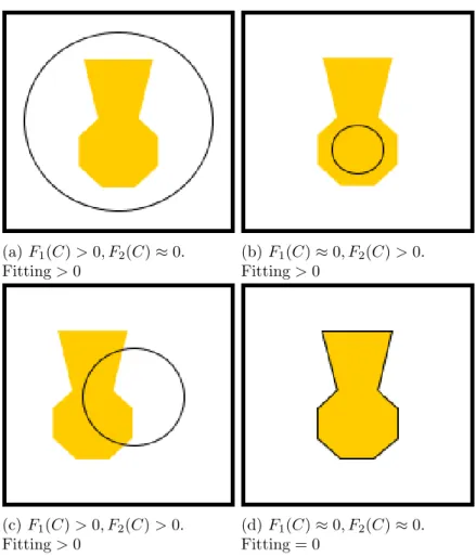
There exists two forces in the Equation (12) : a force to contract the contour and a force to expand the contour. There are four possible positions of the contour C relative to the object to be detected and their corresponding forces as depicted in Figure 4. In case the contour covers the entire object plus some part of its background as shown in Figure 4a, c1 is a little above

0 and c2 is 1 by making an assumption that µi0 = 0 and µo0 = 1. Thus the

sum of area inside the contour minus c1 is greater than 0, while the sum of

area outside the contour minus c2 is equal to 0. This leads to positive

non-zero fitting value and the contour is contracted. Other cases follow similar principle and the contour stops from evolving when both forces equal to zero. This condition holds when the contour lies exactly on the border of the object as depicted in Figure 4d.

(a) F1(C) > 0, F2(C)≈ 0. Fitting > 0 (b) F1(C)≈ 0, F2(C) > 0. Fitting > 0 (c) F1(C) > 0, F2(C) > 0. Fitting > 0 (d) F1(C)≈ 0, F2(C)≈ 0. Fitting = 0

Figure 4: All possible locations of a contour relative to the object and their corresponding fittings

(21)

2.5 Change detection as calving event detector

Change detection is a process of finding a set of pixels having significant diﬀerence from two images capturing the same scene at a diﬀerent time. The method accepts a sequence of two images as input and produces a binary image B(x), referred as a change mask, that shows changed regions based on the following rule [14]:

B(x) = �

1 if significant change exists on pixel or region x

0 otherwise (13)

The existence of changes can be detected using various operations, such as : image diﬀerencing, image rationing, change vector analysis, principal component analysis (PCA), and post-classification comparison [13].

In general, change detection methods can be classified into two categories : pixel-based and object-based. Pixel-based change detection finds changes in multi-temporal images pixel by pixel. In contrast, object-based one de-termine changes by examining the characteristic of regions from the same location from series of images. Pixel-based change detection is known to have serious limitations. It is susceptible to noise and illumination changes since it does not expose local structural information. Therefore, it is not suitable to be implemented in a complex environment. On the other hand, region-based change detection is more stable to handle noise and illumination changes since it relies on local structural features [29]. The most important feature is a texture, which measures variability of neighbouring pixels using mov-ing kernel. Most common textures used in remote-sensmov-ing applications are first-order statistics (standard deviation and skewness) and second-order statistics (Grey Level Co-Occurrence Matrix (GLCM) and semivariance) [30].

2.5.1 Local Binary Pattern (LBP) texture extraction

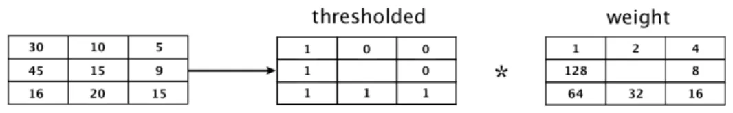
Local Binary Pattern (LBP) is a powerful yet simple texture descriptor. It is very discriminative, less invariant to illumination changes and has a simple representation as well as calculation [31]. LBP was originally developed by Ojala et al. [32] inspired by the Texture Units [33]. The smallest unit of LBP is a 3 x 3 neighbouring grid where the center point gc is the threshold

value. Thresholded values s(x) are produced by comparing the intensity value of a pixel gp in a grid with its center c using the following formula :

s(x) = �

1, gp≥ c

0, gp< c (14)

The descriptor is the result of multiplication of the thresholded value and weight as pictured in Figure 17. LBP value from the example is (1_{∗ 1) +} (16_{∗ 1) + (32 ∗ 1) + (64 ∗ 1) + (128 ∗ 1) = 241.}

(22)

Figure 5: Thresholded value and weight from a 3x3 grid

Ojala et al. extend the basic LBP into LBPP R in [34] by adding a

neigh-borhood radius R and gray levels of P variables. The radius variable R defines the radius of a circular neighborhood set as depicted in Figure 6. By assuming that the center gc is located at (0, 0), the coordinate of a

neigh-boring pixel gp, (p = 1· · · P ) is (−R sin(2πp/P ), R cos(2πp/P )). If the

coordinate is not located in the center of a pixel, the grayscale value of gp

is calculated using an interpolation.

(a) (P=4,R=2.0) (b) (P=8,R=3.0)

Figure 6: Neighborhood map with various P and R.

Similar to its underlying method, the enhanced method forms a texture image by multiplying thresholded values with a weight matrix. However, the latter method assembles the thresholded matrix in a diﬀerent way. It thresh-olds the sign of diﬀerences gp−gcrather than comparing their grayscale

val-ues. Then the diﬀerences are then given binary values based on the following rule :

s(x) = �

1 gp− gc ≥ 0

0 gp− gc < 0 (15)

The weight for each thresholded value is given by a binomial factor 2p, leading to the final LBPP R formula :

LBPP R =

P_�−1 p=0

(23)

2.5.2 Combined diﬀerence change detection

One way to reveal changed pixels from two images is by differencing them using various operators. Two of them are subtraction and ratio operators. The former operator has an ability to expose detail on a weakly change area. Even though it seems to be an advantage, this feature introduces error in an image captured from a noisy environment like the one used in this research. On the other hand, the latter operator can reduce certain amount of noise. However, the operator may produce misleading result since weakly change area and strongly change area are treated the same as long as their ratios are equal. For instance, a pixel with grayscale value of 400 and 200 from two multitemporal images produces ratio of two, while a pixel with weak change having grayscale value of 4 and 2 produces the same ratio. The example emphasizes that single difference operator cannot produce satisfactory result and motivates Zheng et al. [35] to use both of the operators in their method, namely the Combined Difference Image and K-Means clustering (CDI-K).

The CDI-K method generates two separated change masks using subtrac-tion and log ratio operators as shown in Equasubtrac-tion (17) and (18), respectively. It is worth to mention that the grayscale value for log ratio operator is added by one to avoid mathematical error if the pixel value is zero, since log(0) is undefined. After that, the change masks Ds and Dl are normalized to the

range of [0,255]. Ds=|X1− X2| (17) Dl = � � � �log X2+ 1 X1+ 1 � � � � = |log(X2+ 1)− log(X1+ 1)| (18)

Two types of filters are then applied in order to enhance the change masks. A mean filter is applied to the Ds mask to remove isolated pixels.

It is advised that the radius of the mean filter is large enough to remove suﬃcient amount of noise. The second filter, the median filter, is employed to clear isolated pixels away as well as preserve edges from the mask.

The final mask is constructed as a weighted combination of two filtered masks D�_sand D_l�. The aim of combining two masks is to achieve sleekness of D_s� and maintain edge information from D�_l. Weight parameter α > 0 is used to adjust the sleekness and edge preservation trade-oﬀ. The formula used for merging two filtered masks is shown in Equation (19). K-means clustering then judges change and no-change area by segregates the combined mask into two cluster.

(24)

2.5.3 Change mask reconstruction

The result from a change detection method, specifically from the diﬀerencing method, is not likely to form a solid shape as expected to measure an area. Radke et al. [14] point out that the result of a change detection method is likely formed by a set of clustered points rather than solid shapes. One may implement morphological operations for post-processing to connect scattered points into shapes. However, the operations are less preferred since a mask reconstruction method that involves a spatial information produces better result.

Given a set S of finite points in 2D or 3D space, the α-shape method [36] tries to form shapes from those points. We need to limit our discussion to 2D only because our problem lies on a 2 dimensional space. Intuitively, the authors describe the method as carving ice cream problem where the 2D space is represented as ice cream with chocolate chips inside it. Chocolate chips act as points in 2D space. The goal is to carve as much ice cream as possible without touching or removing any chip using a spherical scoop with radius α. The resulted shape will be bordered by circle arcs. The α-shape of S is retrieved by rectifying the arcs into line segments.

In order to define α-shape in a formal way, let α be an arbitrary, but small positive real. The α-hull of S is defined as the set of points which are not situated inside any empty open disk of radius α. An empty open disk is a region in a 2D plane that contains neither its boundary nor any point in S. Similar to the ice cream definition, curves with radius _α1 make up the boundary of an α-hull as represented in Figure 7a. If the curved boundary is replaced by straight lines, the α-shape of S is formed.

(a) α-hull (b) α-shape

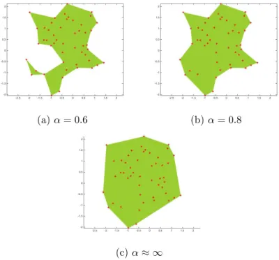
Figure 7: α-hull and its corresponding α-shape from a set of points S Back to its definition, α-shape is defined in a rather vague way since many diﬀerent shapes can be generated from a set of points. In fact, the shape of the points is discriminated by the choice of α. As the α is reduced from 0.8

(25)

to 0.6 from our example depicted in Figure 8b and 8a, the α-shape covers less area because the radius of the empty disk is smaller and occupying more space around the points. If the α is reduced further to zero, the α-shapes are the point themselves. In contrast, if the α is increased towards _∞, the corresponding α-shape is the convex-hull of the points as illustrated in Figure 8c.

(a) α = 0.6 (b) α = 0.8

(c) α≈ ∞

Figure 8: Three polygons reconstructed from the same set of points. The shape of the polygons depends on α value

2.6 Performance assessment for a change detection method

Many researchers evaluate the result of a change detection method based on measures used for evaluating classification performance [37, 38,29,35]. From a comparison between the output of an automated method and a ground truth, which is usually provided by an expert who manually label the data, a confusion matrix is built [39]. The confusion matrix quantifies and categorizes the agreement and disagreement between those two results as depicted in Figure 9 and defined as follows :

• True positives : Number of pixels labeled as changed in both automatic method and ground truth.

• False positives : Number of pixels labeled as changed by a change detection method, but classified as no-change in the ground truth. This measure is also known as false alarms.

(26)

• False negatives : Number of pixel labeled as changed in the ground truth data, but failed to be detected by an algorithm. It is commonly known as missed alarms.

• True negatives : Number of pixels labeled as no-change in both result.

Figure 9: A confusion matrix, comparing human judgment and an automatic classification result.

From a confusion matrix, the following measures are derived :

precision = T P T P + F P (20) recall = T P T P + F N (21) accuracy = T P + T N T P + F N + F P + T N (22)

F-measure = 2_· precision· recall

precision + recall· (23)

The result of change detection method , visually shown as a change mask in Figure 10, presents a condition so-called imbalanced class. In this con-dition, the number of pixels in a class significantly dominate the number of pixels in the other class. Specific to the calving detection case, the number of changed pixels from two consecutive images are significantly fewer than unchanged ones. Kubat et al. [40] underline the inappropriate use of accu-racy measure on imbalance classes. As formulated in (22), huge change in TP does not have big impact on accuracy since TP is significantly fewer than

(27)

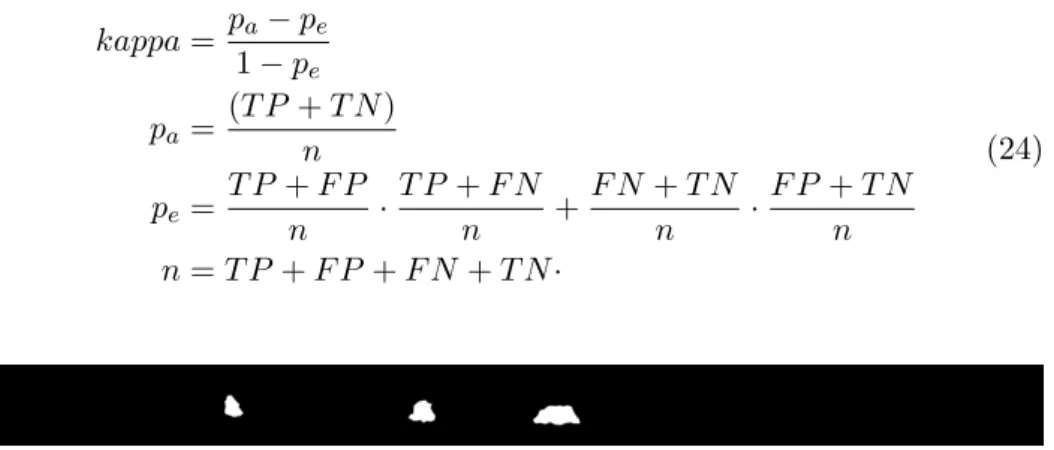
TN. This disadvantage of accuracy has drifted our goal to measure the per-formance of a method to detect changed regions, instead of unchanged ones. They recommend the use of F-measure to measure a classification problem with imbalanced classes. F-measure has a property that is invariant under the change of TN [41], thus it is less sensitive to changes in unchanged pixels. Another alternative to F-measure is Kappa coeﬃcient [42] which measures inter-rater reliability for non-overlapping categorical voting [43]. In this re-search, the first rater is the application while the second rater is human who build the truth data. By referring to a confusion matrix, Kappa coeﬃcient can be formulated as : kappa = pa− pe 1_{− p}e pa= (T P + T N ) n pe= T P + F P n · T P + F N n + F N + T N n · F P + T N n n = T P + F P + F N + T N· (24)

Figure 10: An example of a binary change mask, as a result from a change detection method. White regions represent detected calving regions in a terminus.

(28)

3 Description of the proposed approach

During the execution of the project, a complete framework to detect and measure the area of calving regions is developed. This section explains all details of the framework, starting from the data sets, how an algorithm is adapted, choice of parameters of an algorithm, and evaluation design.

3.1 Data collection

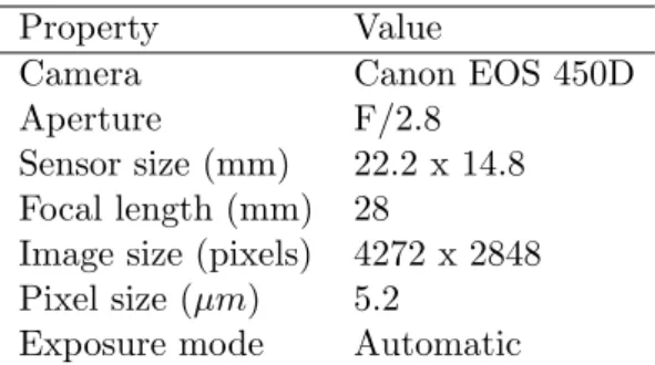
The observation area for this research is focused on Tunabreen glacier in Svalbard, Norway. Doroth´ee Vallot installed a camera in front of the glacier as depicted in Figure 1. A sample image from the data set is shown in Figure 11. The following camera settings and specifications are applied during the image capturing process:

Property Value

Camera Canon EOS 450D

Aperture F/2.8

Sensor size (mm) 22.2 x 14.8

Focal length (mm) 28

Image size (pixels) 4272 x 2848

Pixel size (µm) 5.2

Exposure mode Automatic

Table 1: Camera properties during data collection

In order to capture calving events, the camera was set to capture an image every 14 minutes from 6 July 2014 to 10 September 2014. Due to environmental disturbance like fog and over-illumination, only 413 images taken between 2 September 2014 at 00:05 and 6 September 2014 at 00:13 inclusive are considered as the data set for this project. Based on a manual observation, the selected time frame contains suﬃciently large number of images with minimum environmental noise.

(29)

Figure 11: A sample image from the data set. It shows the terminus of Tunabreen glacier as well as some distracting objects like sea, rocks and mountain

3.2 Implemented methods

In order to achieve the determined goal, several steps are implemented. The framework is started by image registration followed by cropping, segmenta-tion, change detection and area measurement. The flowchart of all building blocks for the framework is depicted in Figure 12 and the detail for each component is explained in Section 3.2.1 through Section 3.2.4

(30)

Figure 12: The flowchart visualizing overall framework

3.2.1 Registration

The first image in a sequence of images is used as reference for the registra-tion process. In other words, all images are registered to the first image in the sequence so all images are geometrically aligned with the same reference. To do that, the SURF-based descriptors of the first image in the sequence are extracted and stored as reference descriptors. The descriptors of each re-maining image (sensed image) are also extracted as input descriptors. In the next step, correspondence information between input and reference descrip-tors are revealed by matching both of them. Based on that correspondence, geometric transformation model that relates sensed and reference images is derived. It is assumed that MSAC uses aﬃne transformation for its baseline model. The final step of registration process is to apply the model to the sensed image.

3.2.2 Cropping

Captured images in the data set as illustrated in Figure 11 contain not only glacier’s terminus but also some distractions such as mountain, sea, rock, and sky. However, calving event to be detected appears only in the terminus. Therefore, only pixels in the terminus area are kept for further process. The first step to extract the terminus area is by cropping the image to a certain dimension. The starting point of the cropping rectangle is (169,1189) in

(31)

Cartesian coordinate and the size is 3911 pixels in width and 443 pixels in height. By using the specified dimension, most of distracting objects are removed as shown in Figure 13. The remaining ones are small part of sea, mountain, glacier top and rock. Cropping is also useful to match the size of the images to the ones from ground truth data used during evaluation process that will be explained later in Section 3.3

Figure 13: Cropped version of Figure 11 focusing on the terminus

3.2.3 Segmentation

The cropping process cannot completely remove non-essential objects. In order to extract the calving terminus from the cropped image, an active contour-based image segmentation method called Chan-vese is applied. The chan-vese algorithm requires an initial mask to separate an object from others. Our application handles that requirement by prompting a user to create an initial mask manually by drawing a rough contour nearby the calving terminus. The user draws the initial mask once and the mask is used as initial mask for all images in the data set. We make an assumption that the registration process works perfectly thus all images are correctly aligned.

The initial mask drawn by the user is iteratively refined to produce a final mask that covers the terminus better. The maximum number of iterations is limited to 50 since we want to reduce computation time. With the limited number of iterations, a user is advised to draw the coarse initial mask as close to the border of a terminus as possible since the accuracy of Chan-vese depends on the initial mask.

The Chan-vese algorithm produces a binary mask, where the background is black (denoted by 0 in Matlab) and foreground is white (denoted by 1). Figure 14 depicts the segmentation result from a single image and for illustrative purpose the final mask and the actual image are blended. There is no guarantee that the final masks from two consecutive images are exactly identical. In contrast, the change detection task in Section 3.2.4 requires pixels from two consecutive images segmented at exactly the same location. To cope with that problem, an image is segmented by a combined final mask. The combined final mask is an intersection of final mask of the current image and that of the previous image. Since both maps are binary, intersection of them is produced by logical operator AND.

(32)

Figure 14: An example of the result of a segmentation process. Terminus area is highlighted by bright mask in a segmented image.

3.2.4 Change detection

The original formulation of the CDI-K change detection algorithm imple-ments K-Means clustering to label pixels into two classes : change and no-change as explained in Section 2.5.2. When we implement CDI-K to detect changes from two images, the clustering step cannot finish after 5 minutes run. We conclude that clustering process is not feasible to judge change and no-change area for our project.

An alternative and still widely used approach to determine a global threshold for change and no-change decision is by using standard deviation of the image’s intensity [44]. Figure 15a presents a change mask from two images having uniform illumination using standard deviation as a thresh-old. In this ideal condition, the CDI (without K-Means) manages to find two visible calving locations. Nevertheless, a brightness change in the terminus because of sunlight reflection from the sea was incorrectly recognized as a change, shown by red dashed rectangle. When illumination is not uniformly spread in an image due to various reasons, standard deviation threshold cannot determine changed and unchanged area correctly, resulting a noisy change mask as pictured in Figure 15b. Calving location cannot be detected from the latter change mask.

(a) Detected changes from image number 9620 to 9621. Green dashed rectangles show actual change while red one shows false detection

(b) Detected changes from image number 9646 to 9647

Figure 15: Detected changes from two consecutive images using standard deviation as the threshold.

Based on the experiment, the global standard deviation threshold does not suitable for a case where the illumination is not uniformly distributed. A variant of thresholding, called local thresholding, is designed to handle the

(33)

situation [45]. The local thresholding computes threshold for every pixel with respect to its neighbor. Significant noise reduction is illustrated in Figure 16 when local threshold with window size of 25 pixels and constant of 0.8 is applied. Although the noise is greatly reduced, the false detection still exists in Figure 16a and calving location is hardly recognized in Figure 16b.

(a) Detected changes from image number 9620 to 9621

Figure 16: Detected changes from two consecutive images using local thresh-old.

An attempt is made to apply the CDI method on top of a texture image instead of a grayscale one. Visual inspection from two successive images reveals that calving events can be identified by textural change instead of intensity change. A texture image is built by applying LBPP R method with

radius of 5 and neighbor set of 8. The result of applying CDI on LBP image is presented in Figure 17. An error caused by a sunlight reflection from the sea does not appear anymore in the Figure 17a. In a image with non-uniformly spread illumination, the method manages to clearly identify the changed area with some minor noises as depicted in Figure 17b.

Figure 17: Detected changes from two consecutive LBP texture images In line with Radke et al.’s theory [14], the change masks as a result of CDI method in Figure 17 consist of scattered points rather than polygons

(34)

representing calving regions. Our method for area measurement as formu-lated in Section 2.2 cannot assess the area of scattered points. To make area measurement possible, clustered points from a change mask are transformed into regions using the α-shape method. The α parameter which control the details of the regions is set to 10. As a last defense from noise, regions hav-ing area less than 100 pixels are considered as noises. Therefore, the region is omitted from the reconstructed change mask. The reassembled change masks are depicted in Figure 18. Some minor noise still appears in Figure 18b.

Figure 18: Reconstructed change masks from two consecutive images

3.3 Evaluation strategy

Ground truth data for the performance evaluation is provided by Pontus Westrin from The Department of Earth Sciences, Uppsala University [15]. He manually marks calving regions by comparing two consecutive images of the terminus of Tunabreen glacier. A confusion matrix is then built based on the definition explained in Section 2.6.

From the confusion matrix, we use false alarms and missed alarms as criteria to evaluate the inaccuracy of the proposed method. To measure the correctness of the method, Kappa-coeﬃcient is more favorable than F-measure. As formulated in (20), (21), and (23), there is a potential where F-measures is undefined due to division by zero. Division by zero arises when precision and recall are zero and one possible cause of zero precision and recall is zero TP. In change detection, a case where either the method or the human or both of them detect no change lead to zero TP. In contrast, the only case where Kappa-coeﬃcient is undefined happens when both rater agree that there is no change between two images. By referring to 24, in this scenario T N = n and T P = F P = F N = 0. Thus, Pa = 0+n_n = 1,

Pe= _n0 ·0_n+_nn·n_n = 1 and Kappa = 1₁−1₋₁ = undefined. In this specific case,

we need to agree that Kappa value is 1 instead of undefined, since both the method and the expert have exactly the same agreement.

The last measure of performance is sourced from estimated area of de-tected calving regions. Area ratio is defined as comparison between the area of calving regions found by the automated change detection to the one found by human observation. It is formulated in (25). Again, there is a possibility

(35)

that area accuracy is undefined due to division by zero problem. If there is a data point in the ground truth data that contains no detected changed region, division by zero occurs. Similar to the previous approach we take, we make an agreement that area comparison equals to zero if either automatic method or human observer found no changes and equals to one if both of them found no changes.

area ratio = area found by automatic method

area found by human observation (25)

The proposed framework is built upon an assumption that there is no environmental noise that may interfere the result. However, the presence of such a noise is ineluctable in real world data sets. That condition holds for our data set where noise appears as for example fog, light reflectance from sea, and significant illumination change between two images. To understand the impact of environment condition on the framework’s performance, we identify the type of noise from two consecutive images. The type of noise is labelled into one of five categories : low illumination change, high illumi-nation change, thin fog, medium fog and thick fog. The decision is made by a human who manually scans all images and put a label into an image. It is worth to mention that in this research we do not make any eﬀort to eliminate a noise as clearly stated in 1.3. The investigation of environmental noise eﬀect is solely made for further development of the framework.

(36)

4 Results

This section displays the result of applying the proposed calving detection and quantization framework to the data set. The experiment is conducted in two stages. The first one uses a portion of data set captured under normal environment condition to see the performance of the framework in accordance with the predefined scope (see 1.3). The second stage evaluates the behavior of the framework under irregular environment.

4.1 Results under normal conditions

Figure 19 shows a change mask between the image captured on 2 September 2014 at 11:31 and the one captured on 2 September 2014 at 11:45. For the rest of this report, this pair of images is referred as normal1. Magenta regions in the mask represent changes detected by human while the green ones show the result of the automatic change detection. Intersection of both regions, the white regions, show the regions marked as changed by both human and computer. The mask shows that most detection errors are contributed by inability of the automatic change detection method to detect changes reported by a human. It is confirmed by much bigger missed alarms compared to false alarms (see Table 2). White regions dominate the change mask, meaning that the method detects calving regions with high precision. Table 2 verifies that by showing Kappa coeﬃcient and area ratio close to 1.

Figure 19: Change mask of normal1 sample images

Another example of images taken under normal condition are the image captured on 4 September 2014 at 15:47 and the one taken 14 minutes later at the same day. This pair of images is referred as normal2. Three calving regions are extracted by the method and fully justified by the expert. A visual inspection reveals that total errors are contributed by missed alarm and false alarm in a similar proportion since the green regions and magenta ones have similar area. It is also proved statistically in Table 2. High accuracy for this sample is indicated by large white area as well as Kappa coeﬃcient and area ratio which approach 1.

(37)

There is a chance that two successive images do not contain calving event at all. The third sample, normal3, from two images taken on 2 September 2014 at 13:51 and the next 14 minutes have no calving regions based on the expert’s judgment. Our application also produces the same conclusion, indicated by a change mask filled with all black. The statistical results, indicated by zero missed alarms and false alarms, Kappa coeﬃcient and area ratio of one, suggest that this special case is handled properly by the method.

Figure 21: Change mask of normal3 sample images.

Change mask in Figure 22 illustrates that the calving region detected by the method does not satisfy the human perception at all, denoted by no intersection between the two regions. The mask is generated based on diﬀerence of an image captured on 3 September 2014 at 10:51 and the one captured 14 minutes earlier. The amount of error is minor, argued by small false and missed alarms. However, the Kappa coeﬃcient goes toward zero since there is no intersection of the result from the method and the one from human interpretation.

Figure 22: Change mask of normal4 sample images.

Table 2: Change detection result for sample images under normal condition

Data False Alarms Missed Alarms Kappa Coeﬃcient Area Ratio normal1 1997 4035 0.8566 0.9062 normal2 1394 2100 0.8826 0.9507

normal3 0 0 1 1

normal4 403 365 -0.0001 0.5672

Figure 23 shows the distribution of Kappa coeffient of images in the data set captured under normal conditions. The distribution suggests that 52.89% of the data have Kappa coefficients below their averages and 25.62% of them have the coefficient greater than 0.7. Figure 26 and Figure 24 depict the distribution of the false alarms and missed alarms, respectively.

(38)

The histograms illustrate that the frequency of false alarms is greatly higher than that of missed alarms. Statistically, the average of missed alarms is 859.7314 while the mean of false alarms is 5198.1.

Figure 23: Distribution of Kappa coeﬃcient under normal conditions.

(39)

Figure 25: Distribution of the most frequent missed alarms under normal conditions.

(40)

Figure 27: Distribution of the most frequent false alarms under normal conditions.

4.2 Results under noisy environment

Results from images in presence of noise is presented in this section. They are divided by the type of noise, as previously discussed in Section 3.3.

4.2.1 Results under minimum illumination

To understand if minimum illumination interferes the performance of the proposed method, the change masks of the two first images captured each day in the data set are presented. Those change masks illustrate the result of change detection from images captured in midnight, where low illumination condition occurs. Note that change mask from 3 September 2014 is excluded since a fog covered the terminus during the midnight.

All images in Figure 28 are distorted by a large number of scattered green regions, meaning that most errors are contributed by false alarms. Despite the intense presence of false alarms, the ability of the method to detect calving regions remains intact. It is shown as white regions in Figure 28b, 28c, and 28d. Table 3 shows a poor result of calving detection, validated by high false alarms, low Kappa coeﬃcient and area ratio that is far from one.

(41)

(a) Change mask of two first images captured on 2 September 2014

(b) Change mask of two first images captured on 4 September 2014

(c) Change mask of two first images captured on 5 September 2014

(d) Change mask of two first images captured on 6 September 2014

Figure 28: Change masks of images captured at midnight

Table 3: Change detection result for sample images under low illumination

Data False Alarms Missed Alarms Kappa Coeﬃcient Area Ratio

a 8636 0 0 0

b 13908 1569 0.3062 3.1610

c 11500 129 0.0834 12.0572

d 6790 826 0.2489 3.929

4.2.2 Results under low illumination change

In order to understand if low illumination change has negative impact to the performance of detection precess, we set a threshold over 5000 false alarms to decide a result is negatively distorted by low illumination change. We also exclude images captured between 00:00 to 05:00 as they have an issue with low illumination condition previously described in Section 4.2.1. From those restrictions, only 8 out of 94 results labeled with low illumination change are negatively influenced by the illumination change. A complete statistic data is provided in Appendix A.

(42)

(a) Change mask with relatively small amount of false alarms.

(b) Change mask of images negatively eﬀected by low illumination change.

Figure 29: Some examples of results under low illumination. Significant amount of noise may appear as the result of low illumination change.

4.2.3 Results under high illumination change

The terminus regions from some images in the data sets encounter major diﬀerence in illumination, either in a certain part or in the entire terminus. Figures 30a and 30b are examples of a pair of two consecutive images having disparity of illumination in a certain region, marked by the red rectangle. Their corresponding change mask (see Figure 30c) shows the location of false alarms, analogous to the location of the region where illumination hikes.

(43)

(a) An image captured under uniform illumination.

(b) An image captured 14 minutes later with a surge of illumination in a part of the terminus. Red rectangle shows the location of the region where illumination increases drastically.

(c) Corresponding change mask from the two images.

Figure 30: Two images with high illumination change and their correspond-ing change mask.

4.2.4 Results in the presence of fog

Based on Table 4 in Appendix A, there are 70 images covered by fog. The intensity of the fog are classified into three categories : thin, medium, and thick. A sample image from the data sets altered by a thick fog is presented in Figure 32. Thin or medium intensity of fog has diﬀerent impact to the magnitude of error. It may emit few regions of false alarm as depicted by Figure 31a and 31c or significant amount of errors as shown in Figure 31b and 31d. Statistically, 56.36% data covered by thin or medium fog have more than 5000 false alarms. On the other hand, images distorted by a thick fog always produces change masks with massive amount of false alarm regions. Two examples of such change masks are presented in Figure 33.

(44)

(a) Change mask from images covered by thin fog. Minimum noise appears.

(b) Change mask from images covered by thin fog. Significant amount of noise appears.

(c) Change mask from images covered by medium fog. Minimum noise appears.

(d) Change mask from images covered by thin fog. Significant amount of noise appears.

Figure 31: Two possible state of noise in a change mask of two images with thin or medium fog.

(45)

(a) First sample of change map of two images covered by thick fog.

(b) Second sample of change map of two images covered by thick fog.

Figure 33: Two change masks of images covered by thick fog. Huge amount of noise appears.

4.3 Overall performance measurement

After presenting some possible causes of errors in calving detection, the performance of the calving detection framework for all images in the data sets is displayed. The distribution of Kappa coefficient shows that 57.039% of it falls below its mean, 0.3188. Only 21.845% of all data has the coefficient greater than 0.7. Figure 34 depicts the distribution of Kappa coefficient.

To identify the most dominant type of errors, histogram of missed alarms and false alarms are displayed in Figure 35 and 37, respectively. The aver-age of false alarms is extremely higher than the averaver-age of missed alarms. Precisely, the average value of false alarms is 16126.9806 while the average value of missed alarms is 817.8301. From those histogram, most missed alarms values lie in the range of 0 - 1800 while the most false alarms values are stretched in a wider and higher range, starting from 0 to 38000.

(46)

Figure 34: Distribution of Kappa coeﬃcient for the entire data set.

(47)

Figure 36: Distribution of the most frequent missed alarms for the entire data set.

(48)

Figure 38: Distribution of the most frequent false alarms for the entire data set.

5 Discussion

This section serves as an analysis of results previously provided in Section 4. In addition, some problems that arise during the experiment are discussed as well.

5.1 Performance and errors

The proposed calving detection framework works well under its defined de-limitation. The method is able to detect calving regions precisely as in-dicated by several measures, such as false alarms, missed alarms, Kappa coeﬃcient, and area ratio. From a geometric point of view, the regions generated by the method have identical shapes as perceived by humans, an indicator that shape reconstruction works well. The results under normal environment conditions reveal that the method hardly detects small calving regions spotted by human eyes, thus missed alarms appear.

The result suggests that the performance of the method is influenced by the presence of a noise in an image. Low illumination, significant illumina-tion change, and thick fog are known to strongly decrease the accuracy of the method. Thin or medium coverage by fog has a fair negative impact on the performance of the method. Meanwhile, small illumination change reduces the performance in rare cases. It is interesting to see that a poor weather condition also decreases human ability to sense calving events. Westrin re-ported that a thick fog greatly reduces the visibility in the terminus [15],

(49)

thus visually marking calving regions is less possible.

The distribution of errors shows that most errors consist of false alarms. As explained in Section 4.3, false alarms are 20 times more frequent than missed alarms. An explanation of the massive amount of false alarms ap-pears in figures in Section 4.2 as a large number of scattered green regions. The figures explains that as some types of noise appear in an image, the method falsely recognized normal regions as calving regions.

5.2 Evaluation technique

Measuring the performance of a change detection method is not a straight-forward task, because some ambiguities exist in the process. We start our discussion with the measures used to assess the performance of the method. False alarms and missed alarms are good indicators for quantifying misclas-sified results of the method. However, those two measures alone cannot judge the performance of the method. Usually, false and missed alarms are employed to compare the result of two or more methods. Since our experi-ment does not compare methods, we decided to rely on the visualization of a change mask rather than statistics. This approach is undoubtedly subjective and may contain some level of inconsistency.

A more accurate result may have been achieved by thresholding missed alarms and false alarms. Any value that falls below the threshold is classified as a good result and vice versa. The threshold should be carefully picked to match a specific problem.

The Kappa coefficient can mislead a reader about the performance of a method. Low value of Kappa coefficient may not indicate low performance of the method. For instance, the normal4 sample image (See Section 4.1) has Kappa coefficient of -0.0001. Based on the Kappa coefficient, we conclude that the method performs poorly in the sample image. However, one can argue that the performance of the method is acceptable based on its change mask as depicted in Figure 22. The change mask presents a limited number of false alarms and missed alarms. In this case, the Kappa coefficient may not be appropriate to show the performance of the change detection method. In order to understand the impact of noise to the performance, the pres-ence of noise in an image is detected visually and then classified into five categories by a person (see Section 3.3). This approach certainly contains some extent of subjectivity. If time permitted, more people were employed to detect a noise in an image and then the overall result is derived based on majority vote of the observers. Another possible way is to use a specific metric representing a type and magnitude of a noise.

(50)

6 Conclusions

A fully automated calving observation framework is an important tool for a geologist to collect more statistical data of calving events. Larger data from long-term observation is needed to understand external factors leading to a calving event, which in the end contributes to global sea level rise. Current development of a long-term calving observation employs a camera to monitor calving terminus and a human to detect the occurrence of a calving. A visual calving detection is prone to be exhausting and time consuming, thus an automatic calving event detector is needed.

A new framework for an automatic calving event detection is presented in this report. The framework is formed based on principle of a change de-tection on top of textural images. More specifically, the combined diﬀerence method is implemented based on Local Binary Pattern texture. Before the change detection is performed, registration and segmentation are conducted. After locations of calving regions are revealed, their corresponding areas are estimated.

Experiments provide important insight into the performance of the pro-posed method. Our method performs well under normal environment con-dition, proved by statistical measures and visual inspection. However, the result of the method starts to be unreliable as a noise appears in an image. Some types of noise influence the method by falsely recognizing unchanged region as calving region. The type of noise triggering false alarms have been successfully identified. Several problems arise as some statistical measures do not clearly reflect the performance of the method. Also, noise labeling tends to be subjective.

6.1 Future work

The main issue found during the experiment is external noise which signifi-cantly reduces the ability of our method to detect calving regions. Therefore, more work should be focused on reducing the eﬀect of noise. A recent dis-cussion with glaciologists from the department of Earth Science, Uppsala University concludes that the use of a laser scanner may reduce the amount of noise in an image since it is less interfered by fog. The laser scanning method can perform a detection process with a higher precision over shorter time-scale but it cannot be deployed for a long time. Fog in an image can also be minimized by taking advantage of the rapid development of haze removal methods.

A low illumination condition can be avoided by finely tuning some cam-era properties, such as shutter speed. A human observer also reports that adjusting luminosity and contrast at several level can help humans spot calv-ing regions better [15]. This finding can be implemented in the framework as well. As a general approach to minimize noise eﬀects, he also suggests