TRITA-LWR.LIC 2028 ISSN 1650-8629
ISRN KTH/LWR/LIC 2028-SE
3-
D NUMERICAL MODELING OF FLOW AND
SEDIMENT TRANSPORT IN RIVERS
Muluneh Admass
TABLE OF CONTENTS ACKNOWLEDGEMENTS ... V ABSTRACT... 1 INTRODUCTION... 1 ECOMSED MODEL ...2 GOVERNING EQUATIONS ...2 Turbulence model... 3 Boundary conditions... 4 NUMERICAL METHODS ...4
MODIFICATIONS AND IMPROVEMENTS...5
The bottom boundary condition... 5
Equivalent sand roughness ... 6
Shear stress partitioning... 6
Bed load transport and bed evolution ... 7
MODEL APPLICATION ...7
Model description and model boundary... 7
Grid generation ... 8 Solution algorithm ... 8 Model calibration... 8 Grid Independence... 8 Sensitivity Analysis ... 9 Validation... 9 Flow field ... 9 Sediment transport ... 10 DISCUSSION ... 10 CONCLUSION ...11 REFERENCES ... 24 iii iii
ACKNOWLEDGEMENTS
First I would like to acknoweledge the Swedish International Development Cooperation Agency (SIDA) for providing me the financial assistance to do my research work. Then I would like to extend my deepest gratitude to my main supervisor Bijan Dargahi, who, with never ending pa-tience, has shared with me his great scientific knowledge and research experience. Assistant su-pervisors Klas Cederwal and Bayou Chane deserve special acknoweledgment. Special thanks to Britt Chow for all her concern and support. Thanks Kirlna for all your sisterly help. I am also very greatful to Hans Bergh, Aira Saarelainen, Nandita Singh, and other colleagues in the vatten-byggnad and in the department of Land and Water Resources, KTH. I am indebted to my spiri-tual father Aba Wolde Meskel, Tin’s family, my family and my friends here in Stockholm and at home. Finally goes all my available thanks to my wife Tin.
Stockholm, May 2005 Muluneh Admass
v v
ABSTRACT
The fully integrated 3-D, time dependant, hydrodynamic and sediment transport numerical model ECOMSED was used to simulate flow and sediment transport in rivers. ECOMSED was originally developed for large water bodies such as lakes and oceans and solves the primitive equations of RANS along with a second order turbulence model in an orthogonal curvilinear σ-coordinate system. The availability of the model as an open FORTRAN source code made modi-fications and addition of new models possible. A new bed load transport model was implemented in the code as well as improvements in treatment of river roughness parameterization, bed form effects, and automatic update of flow depth due to bed evolution. The model was applied to 1-km long reach of the River Klarälven, Sweden, where it bifurcates into two west and east chan-nels. The water surface and the flow division in the channels were made in agreement with field data by spatially varying the roughness. However, the spatial distribution of the bed shear stress was not realistic. Improvements were made in the bottom boundary condition to represent the variable effects of bed forms on roughness depending on the flow regime and the flow depth. The improved model realistically reproduced the flow field as well as the sediment transport processes in the river Klarälven.
Key words: River model; ECOMSED model; River Klarälven; Bed load transport model INTRODUCTION
River modelling applications can be grouped into 2-D depth-averaged hydrodynamic models and 3-D models. An evaluation of the extent to which 3-D models improve predictive ability compared to 2-D models is well described by Lane et al. (1999) and Gessler et al. (1999). They stated that a 3-D model is necessary for predicting sediment erosion and deposition whenever significant secondary currents exist, such as in river bends, crossings, distributaries, or diversions. Some recent research works on flow model-ling are: Weerakoon and Tamai (1989), Olsen and Stokseth (1995), Weiming et al. (1997), Sinha et al. (1998), Lane et al. (1999), Brad-brook et al. (2000), and Chau and Jiang (2001). Olsen and Stokseth (1995) carried out a 3-D simulation of an 80-m long reach of the river Sokna in Norway. The model suc-cessfully predicted the flow features and the results were in good agreement with ob-served data. Sinha et al. (1998) did a compre-hensive numerical study of the flow through a 4-km reach of the Columbia River. They succeeded in modelling both rapidly varying bed topography and the presence of multiple islands. The results agreed well with experi-ments and field measureexperi-ments. In a recent study, Bradbrook et al. (2000) modelled the flow in a natural river channel confluence
using a Large Eddy Simulation (LES). The model simulated periodic flow features in river confluences and agreed well with ex-perimental data. Some recent applications on use of 3-D sediment transport models are: Gesseler et al. (1999), Holly and Spasojevic (1999), Fang (2000), Rodi (2000), Weiming et al. (2000), Nicholas (2001), and Dargahi (2004). Gesseler et al. (1999) applied the U.S. Army Corps Engineering code CH3D-SED to the Deep Draft Navigation project on the lower Mississippi River. The code predicted the sediment deposition in the river with an accuracy of less 13% in comparison with the observations. Holly and Spasojevic (1999) applied and verified the CH3D-SED code to study water and sediment diversion at the Old River Control complex on the lower Mississippi river. Dargahi (2004) predicted secondary flows and the general flow and sediment transport patterns in a river that agreed well with field measurements. A brief review of the major developments in 3-D modeling and the limitations is also given by Lane et al. (2002).
In this paper the fully integrated 3-D, time dependant, hydrodynamic and sediment transport numerical model ECOMSED by Blumberg and Mellor (1987) is used. ECOMSED was originally developed for large water bodies such as lakes and oceans 1
and solves the primitive equations of RANS along with a second order turbulence model in an orthogonal curvilinear σ-coordinate system. The availability of the model as an open FORTRAN source code made modifi-cations and addition of new models possible. The first objective of the present study was to adapt and improve the ECOMSED model for modeling flow and sediment transport in rivers. The second objective was to test the applicability of the improved model to the river Klarälven in the southwest part of Swe-den. A new bed load transport model is im-plemented in the code as well as improve-ments in treatment of river roughness parameterization, bed form effects, and automatic update of bed evolution. The improved model realistically reproduced the flow field as well as the sediment transport processes in the river Klarälven. The secon-dary flows at the river bifurcation and around the bends were well reproduced. The results also agreed well with the previous simulations by Dargahi (2004).
ECOMSED MODEL
The ECOMSED model is a fully integrated 3-D hydrodynamic, wave and sediment transport model. It has a free surface and a bottom following σ-coordinate system (for better representation of irregular bottom topography) with an orthogonal curvilinear grid in the horizontal plane. Here follows a brief description of the governing equations, boundary conditions, the turbulence model and the solution algorithms which are related to the present study. Details of the model can be found in Blumberg (2002).
GOVERNING EQUATIONS
The fundamental equations of fluid dynamics are based on the conservation of mass and momentum. Conservation of mass yields the continuity equation while conservation of momentum yields the momentum equation. Both equations are widely known by Stokes equations. Here follows the Navier-Stokes equations in the Cartesian coordinate system (x,y,z axis). 0 = ∂ ∂ + ∂ ∂ + ∂ ∂ z w y v x u (1a-d) ⎟⎟ ⎠ ⎞ ⎜⎜ ⎝ ⎛ ∂ ∂ + ∂ ∂ + ∂ ∂ + ∂ ∂ − = ∂ ∂ + ∂ ∂ + ∂ ∂ + ∂ ∂ 2 2 2 2 2 2 1 z u y u x u x p z u w y u v x u u t u υ ρ ⎟⎟ ⎠ ⎞ ⎜⎜ ⎝ ⎛ ∂ ∂ + ∂ ∂ + ∂ ∂ + ∂ ∂ − = ∂ ∂ + ∂ ∂ + ∂ ∂ + ∂ ∂ 2 2 2 2 2 2 1 z v y v x v y p z v w y v v x v u t u υ ρ g z w y w x w z p z w w y w v x w u t u + ⎟⎟ ⎠ ⎞ ⎜⎜ ⎝ ⎛ ∂ ∂ + ∂ ∂ + ∂ ∂ + ∂ ∂ − = ∂ ∂ + ∂ ∂ + ∂ ∂ + ∂ ∂ 2 2 2 2 2 2 1 υ ρ
In which are the velocity components
along w v u ,, z y x, , directions respectively, t is time, ρ is the fluid density, is the pressure, p
υ is the fluid kinematic viscosity and is the gravitional force. The flow is assumed in-compressible (constant density) and the fluid’s coefficient of viscosity is taken con-stant. It is possible to solve the Navier-Stokes equations by direct numerical simulation (DNS) if we can resolve all the relevant length scales which vary from the smallest eddies to scales on the orders of the physical dimensions of the problem domain. For channel flow the number of grid points needed to resolve all the relevant scales can be estimated from the expression (Tannehill et al. 1997)
g
(
)
9/4 088 . 0 h e DNS R N = (2) In whichhis the Reynolds number based
on the mean channel velocity and channel height. This approach is limited to flows of simple geometry and very low Reynolds number. Another promising approach is known as large-eddy simulation (LES), in which the large-scale structure of the turbulent flow is computed directly and only the effects of the smallest (subgrid-scale) and more nearly isotropic eddies are modeled. The computa-tional effort required for LES is less than that of DNS by approximately a factor of 10 using present-day methods. The main thrust of present-day research in computational fluid dynamics is through the time averaged Navier-Stokes equations also known as the Reynolds averaged Navier-Stokes (RANS) equa-tions. These equations are derived by de-composing the dependent variables in the conservation equations in to time-mean (ob-tained over an approximate time interval) and fluctuating components and then time aver-aging the entire equation (Tannehill et al. 1997). Time averaging the equations of
mo-e
tion gives rise to new terms, which can be interpreted as “apparent” stress gradients associated with the turbulent motion. ECOMSED model solves the RANS equa-tions with the hydrostatic assumption and the three-dimensional equation describing the advection and diffusion of sediment particles given below, 0 = ∂ ∂ + ∂ ∂ + ∂ ∂ z W y V x U (3a-e) ⎟ ⎠ ⎞ ⎜ ⎝ ⎛ − ∂ ∂ ∂ ∂ + ⎟⎟ ⎠ ⎞ ⎜⎜ ⎝ ⎛ − ∂ ∂ ∂ ∂ + ⎟ ⎠ ⎞ ⎜ ⎝ ⎛ − ∂ ∂ ∂ ∂ + ∂ ∂ − = ∂ ∂ + ∂ ∂ + ∂ ∂ + ∂ ∂ ' ' ' ' ' ' 1 u w z U z u v y U y u u x U x x P z U W y U V x U U t U υ υ υ ρ ⎟ ⎠ ⎞ ⎜ ⎝ ⎛ − ∂ ∂ ∂ ∂ + ⎟⎟ ⎠ ⎞ ⎜⎜ ⎝ ⎛ − ∂ ∂ ∂ ∂ + ⎟ ⎠ ⎞ ⎜ ⎝ ⎛ − ∂ ∂ ∂ ∂ + ∂ ∂ − = ∂ ∂ + ∂ ∂ + ∂ ∂ + ∂ ∂ ' ' ' ' ' ' 1 v w z V z v v y V y v u x V x y P z V W y V V x V U t V υ υ υ ρ z P g ∂ ∂ − = ρ ⎟ ⎠ ⎞ ⎜ ⎝ ⎛ − ∂ ∂ Γ ∂ ∂ + ⎟⎟ ⎠ ⎞ ⎜⎜ ⎝ ⎛ − ∂ ∂ Γ ∂ ∂ + ⎟ ⎠ ⎞ ⎜ ⎝ ⎛ − ∂ ∂ Γ ∂ ∂ = ∂ − ∂ + ∂ ∂ + ∂ ∂ + ∂ ∂ ' ' ' ' ' ' ) ( c w z C z c v y C y c u x C x z C W W y VC x UC t C s
In which are mean velocity
compo-nents in the W V U, , z y x, , directions respectively ( is the main flow direction, is the stream wise direction, is vertical to the bed) while are the corresponding fluctuating velocity components, C is the mean sediment
concentration and is the flactuating com-ponent, Γis sediment diffusivity and is the
settling velocity of sediment particles. The new correlations that appeared in the above equations are related with the mean values using turbulence models. The settling velocity of sediment particles is calculated from the effective diameter of the suspended sediment using the semi-empirical formulation of Cheng (1997) x y z ' ' ' , ,v w u ' c s W
(
)
[
]
1.5 5 2 . 1 25 *20.5 50 − + = D D Ws υ (4) 50 3 / 1 2 * ) 1 ( D g s D =⎢⎣⎡ − ⎥⎦⎤ υ (5)In which is particle diameter for 50%
finer of bed material, * is the dimensionless grain size and is specific density.
50
D
D
s
Turbulence model
Turbulence models are used to relate the new correlations that appeared in the RANS equa-tions and in the mean sediment concentra-tion equaconcentra-tion with mean values or in other words to close the system of equations. Here follows the description of equations used in ECOMSED to relate the new correlations with the mean values.
(
)
(U V) z K v w u w' ', ' ' M , ∂ ∂ = − (6a-d)(
)
⎟⎟ ⎠ ⎞ ⎜⎜ ⎝ ⎛ ∂ ∂ ∂ ∂ = − x U y V A v v u u , 2 M , ' ' ' ' ⎟⎟ ⎠ ⎞ ⎜⎜ ⎝ ⎛ ∂ ∂ + ∂ ∂ = − = − x V y U A u v v u M ' ' ' '(
)
⎟⎟ ⎠ ⎞ ⎜⎜ ⎝ ⎛ ∂ ∂ ∂ ∂ ∂ ∂ = − z C K y C A x C A c w c v c u , , H , H , H ' ' ' ' ' 'In which Mis the eddy viscosity, KHis the
eddy diffusivity, Mis the horizontal viscosity and is the horizontal diffusivity. The horizontal viscosity M is calculated accord-ing to Smagorinsky (1963) K A H A A 2 1 2 2 2 1 ⎥ ⎥ ⎦ ⎤ ⎢ ⎢ ⎣ ⎡ ⎟ ⎟ ⎠ ⎞ ⎜ ⎜ ⎝ ⎛ ∂ ∂ + ∂ ∂ ∆ = i j j i M x U x U c A (7)
In which c = 0.01, ∆2 = ∆x∆y, and Einstein
convention is used. ∆x and ∆y are the grid spacing in the x and y directions respectively. The horizontal diffusivity His usually set equal to M. Mand Hare obtained by
ap-pealing to a second order turbulence closure scheme developed by Mellor and Yamada (1982) which characterizes the turbulence by equations for the turbulence kinetic energy,
A
A K K
2
2 1
q , and turbulence macroscale, l ,
accord-ing to, ⎟⎟ ⎠ ⎞ ⎜⎜ ⎝ ⎛ ∂ ∂ ∂ ∂ + ⎟⎟ ⎠ ⎞ ⎜⎜ ⎝ ⎛ ∂ ∂ ∂ ∂ + − ⎥ ⎥ ⎦ ⎤ ⎢ ⎢ ⎣ ⎡ ⎟ ⎠ ⎞ ⎜ ⎝ ⎛ ∂ ∂ + ⎟ ⎠ ⎞ ⎜ ⎝ ⎛ ∂ ∂ + ⎟⎟ ⎠ ⎞ ⎜⎜ ⎝ ⎛ ∂ ∂ ∂ ∂ = ∂ ∂ + ∂ ∂ + ∂ ∂ + ∂ ∂ y q A y x q A x B q z V z U K z q K z z q W y q V x q U t q H H M q 2 2 1 3 2 2 2 2 2 2 2 2 2 l (8a,b) ( ) ( ) ( ) ( ) ( ) ⎟⎟ ⎠ ⎞ ⎜⎜ ⎝ ⎛ ∂ ∂ ∂ ∂ + ⎟⎟ ⎠ ⎞ ⎜⎜ ⎝ ⎛ ∂ ∂ ∂ ∂ + − ⎥ ⎥ ⎦ ⎤ ⎢ ⎢ ⎣ ⎡ ⎟ ⎠ ⎞ ⎜ ⎝ ⎛ ∂ ∂ + ⎟ ⎠ ⎞ ⎜ ⎝ ⎛ ∂ ∂ + ⎟⎟ ⎠ ⎞ ⎜⎜ ⎝ ⎛ ∂ ∂ ∂ ∂ = ∂ ∂ + ∂ ∂ + ∂ ∂ + ∂ ∂ y l q A y x l q A x W B q z V z U K E z q K z z q W y q V x q U t q H H M q 2 2 1 3 2 2 1 2 2 2 2 2 ~ l l l l l l
In which are empirical
constants. The wall proximity function, W
q S E E B B A A1, 2, 1, 2, 1, 2, ~, is defined as 3
2 2 1 ~ ⎟ ⎠ ⎞ ⎜ ⎝ ⎛ + = L E W κl (9) z H z L= − + + 1 1 1 η (10)
In which κis the von Karman constant, ηis the water surface elevation and H is the
water depth. While details of the closure module are rather involved, it is possible to reduce prescription of the mixing coefficients to the following expressions,
3 / 1 1 B q KM = l (11a-c) ⎟⎟ ⎠ ⎞ ⎜⎜ ⎝ ⎛ − = 2 1 2 6 1 B A qA KH l q q qS K =l
Empirical constants are
respectively (Mel-lor and Yamada 1982).
q S E E B B A A1, 2, 1, 2, 1, 2, 2 . 0 , 33 . 1 , 8 . 1 , 1 . 10 , 6 . 16 , 74 . 0 , 92 . 0 Boundary conditions
The boundary conditions are specified as surface, bottom and open boundaries.
Free surface: The boundary conditions at the free surface,z=η(x,y,t), are
(ox oy) (12a-e) M z V z U K τ τ ρ , ⎟= , ⎠ ⎞ ⎜ ⎝ ⎛ ∂ ∂ ∂ ∂ 2 3 / 2 1 2 s u B q = τ 0 2 = l q t y V x U W ∂ ∂ + ∂ ∂ + ∂ ∂ = η η η 0 = ∂ ∂ z C KH
In which
(
τox,τoy)
is the surface wind stressvector with the surface friction velocity, , being the magnitude of the vector.
s
uτ Bottom boundary: The boundary conditions at bottom boundary,z=H(x,y), are
(
)
(13a-e) by bx M z V z U K τ τ ρ , ⎟= , ⎠ ⎞ ⎜ ⎝ ⎛ ∂ ∂ ∂ ∂ 2 3 / 2 1 2 b u B q = τ 0 2 = l q y H V x H U Wbt bt bt ∂ ∂ − ∂ ∂ − = D E z C KH = − ∂ ∂In which are the velocity
compo-nents at the bottom,
bt bt bt V W U , , D E− is the sediment
flux at the water sediment interface which is calculated using the van Rijn (1984a) proce-dure and is the bottom friction velocity associated with the bottom frictional stress
b
uτ
(
τbx,τby)
. In ECOMSED the bottomstress is determined by matching velocities with the logarithmic law of the wall.
b b D
b ρC V V
τ = (14)
With the value of the drag coefficient CD given by 2 ln 1 − ⎥ ⎦ ⎤ ⎢ ⎣ ⎡ ⎟⎟ ⎠ ⎞ ⎜⎜ ⎝ ⎛ + = o b D z z H C κ (15)
In which and are the grid point and
corresponding resultant horizontal velocity in the grid point nearest to the bottom. The
parameter depends on the local bottom
roughness.
b
z Vb
0
z
Open lateral boundary: Two types of open boundaries exist, inflow and outflow. The normal component of velocity is specified while a free slip condition is used for the tangential component at inflow boundaries. Turbulence kienetic energy and the macro-scale quantity ( ) are calculated with suffi-cient accuracy at the boundaries by neglecting the advection in comparison with other terms in their respecttive equations. The sediment concentration data at the inlet is specified, whereas at outflow boundaries the mixed boundary condition is used. The clamped boundary condition in ECOMSED allows assigning observed water level along the open boundary grids.
l q2
NUMERICAL METHODS
The governing equations and boundary con-ditions are transformed in to a vertical σ- layer and an orthogonal curvilinear horizontal (ξ1ξ2) coordinate system. The σ- transforma-tion is given by η η σ + − = H z (16)
In which η is the water surface elevation. The vertically and horizontally transformed set of equations is approximated by a finite
difference scheme using a spatially staggered grid. The leap frog scheme with the Cou-rant-Friedrichs-Levy (CFL) computational stability condition and a weak filter to re-move solution splitting at even and odd time steps is employed for time differencing. Three options (upwind difference, central difference and Multidimensional Positive Definite Advection Transport Algorithm) are available for spatial differencing. The hydro-dynamic module (ECOM) is 3-D with a split external-internal mode algorithm; the exter-nal mode explicitly solves the depth inte-grated equations with short time steps to resolve fast moving waves and to determine the water surface elevation. The internal mode uses the computed water surface eleva-tion and implicitly solves the vertical struc-ture of the flow with a shorter time step. The internal mode then updates some of the variables of the external mode for the next time step to begin. At regular intervals speci-fied by the user the sediment transport mod-ule (SED) which uses the same numerical grid, structure and computational framework as the hydrodynamic model simulates sedi-ment resuspension, transport and deposition of cohesive and non-cohesive sediments using the previously computed hydrodynamic variables.
MODIFICATIONS AND IMPROVEMENTS
The application of ECOMSED to rivers can be improved by considering some of the specific features of river hydraulics that dif-fers from large scale motions such as rough-ness, spatial variations of flow depth, and bed load transport. In rivers, significant variations in channel and river bed roughness are found. Furthermore, the formation of bed forms directly affects the resistance to flow as well as the distribution of bed shear stresses. The other aspect is the spatial variation of the flow depth that affects the velocity distribu-tion and the boundary layer characteristics. In ECOMSED model a constant roughness value is used. The effect of bed form rough-ness which depends on the local flow regime is not considered. The bed load transport is also not modeled. To implement the
forgo-ing aspects in the model the river Klarälven was used as a case study. Realistic and com-parable results with field measurements and with previous simulations using other models were obtained after the following improve-ments and modifications were made.
The bottom boundary condition
The bottom boundary condition used in ECOMSED as given in equations (14) and (15) is the generalization of the logarithmic law which assumes the same roughness in the whole computational domain. However, in rivers roughness which is composed of skin friction due to bed grains and drag form due to bed forms varies spatially and temporally depending on the local flow depth and the local flow regime. The bottom boundary condition was reformulated as follows to directly represent the spatial and temporal variation of the bottom roughness. Starting from the general equation of the logarithmic universal velocity distribution (Schlichting 1968) B B u z H u Vb b ∆ − + ⎟ ⎠ ⎞ ⎜ ⎝ ⎛ + = υ κ * * ) ( ln 1 (17)
In whichB=5.45, κ =0.41 and∆B, the
rough-ness induced velocity deficit is a function of the equivalent roughness heightks. Denoting
υ
/
*
u
ks by and using the interpolation
for-mula by Cebeci and Bradshaw (1977) + s k [ ] { } ⎪ ⎪ ⎪ ⎩ ⎪ ⎪ ⎪ ⎨ ⎧ > + − ≤ ≤ − ⎥⎦ ⎤ ⎢⎣ ⎡ − + < = ∆ + + + + + + 90 ln 1 5 . 8 90 25 . 2 811 . 0 ln 4258 . 0 sin ln 1 5 . 8 25 . 2 0 s s s s s s k k B k k k B k B κ κ (18)
Using equation (17) and (18) the roughness parameter in equation (15) becomes z0
κ υ ) ( * 0 B B e u z = −∆ (19)
Equation (19) allows specifying spatially and temporally variable roughness depending on the velocity deficit ∆B which is a function of
the local equivalent sand roughness and the local shear Reynolds number as shown in equation (18). Available empirical formulas were used to compute the equivalent sand roughness of bed grains and bed forms as 5
described in the next section. Further modifi-cation was done to solve the problem of locating the last grid in the narrow range of the logarithmic region in highly variable river bed topography. This can be described as follows. The logarithmic law defined by equa-tion (17) is valid approximately in the range40υ ( ) 0.2δ * ≤ + ≤ H zb u where δ is the thickness of the boundary layer. Since ECOMSED uses the same number of verti-cal grids, the validity of the logarithmic law requires the depth,(H +zb), which is half
depth of the last σ- layer to be located within the logarithmic region throughout the whole computational domain. In rivers as there are high spatial and temporal variations in flow depth and flow regime satisfying the validity limits everywhere in the computational do-main is difficult if not impossible. One possi-ble approach is to use a universal velocity distribution law which is valid for the whole flow depth. The validity of the logarithmic region can be extended to the whole flow depth by using the velocity defect law (Coles 1956), given by equation (20). ( ) ⎟ ⎠ ⎞ ⎜ ⎝ ⎛ + Π + ∆ − + ⎟ ⎠ ⎞ ⎜ ⎝ ⎛ + = δ κ υ κ b b b H z f B B u z H u V * * ln 1 (20)
In which Π is the profile parameter
and ( )
δ b z H
f + is the wake function. The
boundary layer thickness can be computed from equation (21) for known values of free
stream velocity, and the distance
(Schlichting 1968). ∞ U l 5 1 37 . 0 − ∞ ⎟ ⎠ ⎞ ⎜ ⎝ ⎛ = υ δ l U l (21)
For rivers equation (21) is difficult to evaluate as the velocity profiles could be skewed due to 3-D effects and the flow field may contain many flow separated regions. For practical applications the boundary layer thickness can be assumed to be related to the flow depth, i.e., δ =βH. A new expression for can be
obtained from equation (20) for the wake law with an empirical fit to the wake function given by Cebeci & Bradshaw (1977)
0 z ⎟⎟ ⎠ ⎞ ⎜⎜ ⎝ ⎛ ⎟⎟ ⎠ ⎞ ⎜⎜ ⎝ ⎛ + − Π − ∆ − − = H z H B B b e u z β π κ υ ( ) 1 cos * 0 (22)
For a given set of σ- layers equation (22) needs a minimum depth to be set so that the first grid off the bed surface lies above in the whole computational domain.
0
z
Equivalent sand roughness
Equivalent sand roughness is composed of grain, saltation and bed form roughness. The component of roughness due to saltation and bed forms depends on the local flow depth and local flow regime. As a result, the equiva-lent sand roughness in rivers varies both in space and time. The problem is how to de-lineate the areas where the bed forms are contributing to the resistance and where they are not. Generally the van Rijn’s (1984b) procedure can be used to identify the local bed forms and the corresponding equivalent sand roughness depending on the dimen-sionless grain size and transport stage pa-rameter. In this study the average observed energy gradient and the critical shear velocity for the average bed grain size of the river were used to compute the ‘critical’ flow depth below and above which we have only grain roughness. A polynomial fit was then used to smooth out the spatial distribu-tion of the neighboring cells around the ‘critical’ flow depth. The grain roughness was
taken as . Wiberg and Rubin (1985)
sug-gested the saltation roughness in terms of value to be approximately 0.1 cm. Field studies showed that the river bed for the test case of this study is composed of three di-mensional ripples and the equivalent bed roughness due to ripples was calculated ac-cording to Grant and Madsen (1982)
0 z 90 3D 0 z λ 2 7 . 27 ∆ = s k (23)
In which ∆ is bed form height and λis bed form length.
Shear stress partitioning
The other modification made was shear stress partitioning (in areas where bed form is contributing to flow resistance) to extract the
effective part of the stress that contributes to sediment transport. The effective shear ve-locity, , for the lower flow regime (ripples and dunes) was calculated by using the flow resistance relationship by Engelund and Hansen (Yang 1996). ' * u 5 . 0 50 4 * 50 ' * ) 1 ( 4 . 0 ) 1 ( 06 . 0 ⎟⎟ ⎠ ⎞ ⎜ ⎜ ⎝ ⎛ − + − = D s g u D s g u (24)
The transport stage parameter, Twhich is
used for the computation of suspended and bed load was calculated using this effective shear velocity (van Rijn 1984a and van Rijn 1984b)
( )
(
)
(
)
2 *, 2 *, 2 ' * crbed crbed u u u T= − (25)In which is the critical bed shear ve-locity which depends on the local shear Rey-nolds number and was calculated using the Shields curve for initiation of motion. The critical shear velocity was also corrected for the bottom and side slopes according to Chien (1999).
crbed
u*,
Bed load transport and bed evolution In rivers the contribution of bed load trans-port to the total load can be significant. Thus a realistic modeling of sediment transport would require the inclusion of the bed load transport. This was done by including the bed load in the sediment mass-balance equa-tion for the bed evoluequa-tion.
0 ) 1 ( 2 1 2 1 = ∂ ∂ + ∂ ∂ + − + ∂ ∂ − ξ α ξ αbξ b bξ b b q q D E t z p (26)
In which is the actual bed load transport, is the porosity of the bed material,
b q p 1 ξ αb and 2 ξ
αb are the direction cosines in the or-thogonal curvilinear coordinates ξ1 and
2
ξ respectively. A formulation for the bed deformation (Rodi 2000) was used.
(
*)
1 ) 1 ( b b s b q q L t z p = − ∂ ∂ − (27)The equilibrium bed load transport, *and the non-equilibrium adaptation length for bed load transport, L
b
q
s were calculated
accord-ing to van Rijn (1984a)
[
]
0.3 * 1 . 2 5 . 1 50 5 . 0 * 0.053( 1) D T D g s qb = − (28) 9 . 0 6 . 0 * 50 3D D T Ls = (29)Substituting equation (27) in equation (28) produces an elliptic equation. First order upwind scheme discretization of the resulting equation produces a tri-diagonal matrix which was solved using the modified strongly implicit procedure of Stone (1968). The bed evolution was evaluated using the leap-frog method using equation (27). The depth of the water was then adjusted according to the changes in the bed so that the flow field can respond to the new situation.
MODEL APPLICATION
The improved model was applied to a test case, the river Klarälven.
Model description and model boundary The river Klarälven enters Sweden in the north of the county of Värmland. Its course in Värmland is south down to the river mouth on lake Vänern at the city of Karlstad where it bifurcates into an east and west channels. Vänern is the largest freshwater lake in Sweden. The course of the river is a sequence of regular meanders that are unique with respect to size and regularity. A one kilometre long reach of the river was mod-elled that extends 0.5 km upstream of the bifurcation (Figure 1). To insure uniform inlet boundary conditions, the upper limit of the reach was placed in a straight river sec-tion. The river topography was measured in April 2004 at 11312 points scattered along the river reach. The mean measurement resolution ranges from 2 m to 6 m. The flow discharges at the inlet and the two outlets defined by east and west channels were measured. Point velocity measurements were also taken at the inlet at 10 m intervals across the stream and at 0.5 m intervals in the verti-cal direction. To define the inlet boundary conditions, the velocities along a vertical at each station were fitted to the wake law ve-locity distribution to obtain the bed shear velocity. A continuous distribution of the bed shear velocity across the stream was obtained by fitting a curve to the bed shear velocities 7
calculated for each station. The velocity at different σ-layers for each computational inlet grid was then computed using the wake law velocity distribution with the shear veloc-ity at the same grid. The observed water levels at the outlet of the east and west chan-nels were specified. River bottom above the observed water surface was considered as dry or inactive cell. Flow depths less than 0.2 m were considered as 0.2 m to avoid instabilities due to sediment deposition. At the inlet and outlet boundaries equilibrium bed load was assumed while zero suspended sediment concentration was used at the inlet boundary as sediment load data was not available. Grid generation
The numerical model was built using the interpolated bottom topography (Figure 1). The horizontal orthogonal curvilinear grid was generated by CCHE2D mesh generator using the Poisson scheme with smoothness and orthogonality of 91 and 95 %, respec-tively. The average grid spacing in the com-putational domain was about 6.0 m. The grid spacing around the bifurcation and around the bends was made finer with an average spacing of 2.0 m.
Solution algorithm
In this study, data for discharge hydrograph was not available and the flow simulation was done for an observed steady flow of 285 m3/s which lasted for 2 hours. The model
was run with time steps of 0.2 seconds for the internal mode and 0.02 seconds for the external mode with a ramping of 10000 steps. The model was restarted and run for extra steps until steady state flow field was ob-tained. The sediment transport was then activated and the model was run for 2 hours. Model calibration
The model was calibrated for a discharge of 285 m3/s using the measured water surface
profiles and discharge division between the two river channels. The percentage of the discharge into west and east channels were 42% and 58%, respectively. Model calibration was done for a grid number of 126x48x9 by spatially varying the roughness to satisfy both
the water division and the water surface profile. The normalized error in the com-puted flow division was with in 0.8 % (West channel) and 0.6 % (east channel) while the normalized error in the water surface varied with in 0.14 % in the deep areas to 3 % in the shallow areas.
Grid Independence
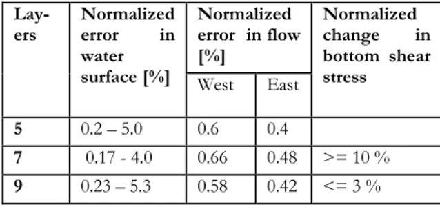
A grid dependency study was carried out to minimize numerical errors due to coarse discretization. In the horizontal direction the number of grids was dictated by the available resolution of the bottom topography. Five vertical layers were taken to start with. By spatially varying the roughness the normal-ized error in the water surface profile was made to lie within 0.2 to 5 % and the flow division was 0.6 % in the west channel and 0.4 % in the east channel. The number of grids in the vertical direction was increased from 5 to 7. By using the same roughness distribution used for 5 layers the normalized error in the water surface profile was within 0.17 to 4 % and the flow division was 0.66 % in the west channel and 0.48 % in the east channel. There was no significant change in the water surface profile and flow division. However, the change in the shear stress was very significant (the normalized change be-tween the shear stress fields of 5 and 7 layers was about 10 % and greater). When the number of grids was increased to 9 the nor-malized shear stress change between 7 and 9 layers was less than 3%. The results are summarized in Table 1. Thus, the resolution 126x48x9 is sufficient to obtain reliable nu-merical results.
Table 1. Table showing the change in the normalized errors and shear stress as the number of vertical layers is increased.
Normalized or in flow [%]
err
Lay-ers Normalized error in water
surface [%] West East
Normalized change in bottom shear stress 5 0.2 – 5.0 0.6 0.4 7 0.17 - 4.0 0.66 0.48 >= 10 % 9 0.23 – 5.3 0.58 0.42 <= 3 %
Sensitivity Analysis
Sensitivity analysis was made to check how far simulation results were sensitive to bed roughness used for calibration. The water surface difference between the inlet and the outlet was found to vary approximately line-arly with the roughness while the flow divi-sion in the east and west channel was found not sensitive to changes in roughness. Suc-cessively increasing the roughness from a
value of 1 cm to 2 cm and to 3 cm pro-duced an average water surface gradient of 0.007 %, 0.01% and 0.013%, respectively. However, the bottom shear stress was found to be very sensitive to the change in the roughness. A similar increment of roughness from a value of 1 cm to 2 cm produced a spatial bottom shear stress variation of up to 40 %. 0 z 0 z Validation
A comprehensive validation of the model would require extensive field data on water surface profiles, velocity profiles, secondary flow structures and flow circulation regions. For the purpose of this study only limited data were available at two different discharge values of 285 m3/s and 136 m3/s. The model
was validated with the field data for 136 m3/s
by using the roughness distribution obtained during calibration for 285 m3/s. In
compari-son with field data, the normalized error in the observed water surface profile varied from 0.11 % to 1.33 %. The normalized error in the flow division was 2.44 % for the west channel and 1.56 % for the east channel. Regarding the flow field, stream lines as well as the local flow circulation region upstream of the river bifurcation agreed well with the field observations (Figure 2). The predicted secondary flow fields also showed a general agreement with the previous simulations done by Dargahi (2004).
Flow field
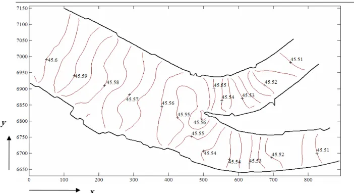
The flow field in the river was successfully simulated by the model that included the water surface profiles, velocities, secondary flows, and bed shear stresses. Figure 3 shows the contour lines of the water surface
pro-files. At the bifurcation point (stagnation) the local increase in water surface elevation is shown. The model also predicted the trans-verse water-surface slope at the river bend in agreement with the physics of the helicoidal secondary flows. The water surface su-perelevation depths between the outside bank and inside bank ranged between 5 to 8 mm in the east channel bend and from 3 to 9 mm in the west channel bend. They were comparable to approximate values of 7 mm (East channel) and 8 mm (west channel) computed using lppen and Drinker (1962) method.
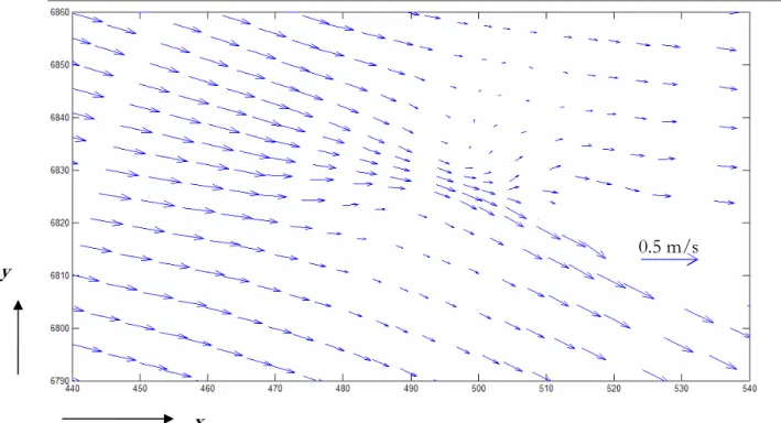
The velocity vectors closely followed the bed topography. A general flow diversion from the main channel to the east channel was detected that explains the large portion of the total flow entering the east channel. The flow field showed horizontal secondary flows following the river banks at locations where the river topography forces flow separations to occur. The examination of the velocity vectors and velocity contours in different horizontal planes showed that the flow sepa-ration regions had a complex 3D form that extended from the water surface to the river bed. The velocity vectors upstream of the bifurcation also showed a significant varia-tion with the depth. The surface velocity vectors (Figure 4) showed no secondary flows apart from flow line convergence due to the local increased in the depth. However, from the fourth sigma layer downwards large flow recirculation regions appeared (Figures 5 and 6).
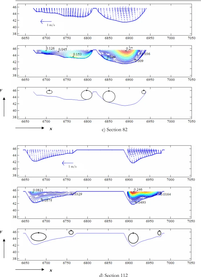
The general patterns of the secondary flows in the vertical directions were predicted by the model. Few examples are given in Fig-ures 7(a-d) where the velocity vectors, veloc-ity contours and the interpolated secondary flows are shown. The velocity contours for different layers are given in figures 8(a-h) to show the general pattern of velocity variation in the vertical direction. The bed shear stresses were computed as total as well as effective stresses, Figures 9 and 10 showing the two cases, respectively. The distributions of shear stresses are similar for both cases although the magnitudes of total shear stresses are about four times higher than the 9
effective shear stresses. As the bed shear stress is the primary agent for sediment transport, the difference in magnitude is important. The results emphasis the need of choosing an appropriate distribution for sediment transport computations. In com-parison with west channel, the shear stresses are higher in the east channel as well as in the deep main channel that conveys a larger portion of the flow into the east channel. The lower shear stress regions correspond to the area with little sediment transport activities. Sediment transport
The general pattern of bed changes after 2-hours is shown in Figure 11. The figure shows the contour lines expressed in the units of millimeter (erosion in negative sign). The main features are the formation of a sandbank at the entrance to the east channel and the division of the main channel into two regions of erosion and deposition. The model predicted the classical erosion patterns ob-served in the river bends. The maximum erosion depth was -46.7 mm, which occurred in the east channel near the concave curve. A similar trend was found in the west channel bend although the maximum erosion was -20 mm. The high values correspond to the re-gions of high effective bed shear stresses. Figures 12(a-d) compare the predict bed level changes at 3 representative river cross sec-tions. For the ease of comparison the verti-cal sverti-cale corresponding to the model values are exaggerated. The division of river into distinct regions of deposition and erosion are well illustrated by these figures.
DISCUSSION
Flow field: The direct application of the ECOMSED model with no modifications caused a number of difficulties that produced unrealistic results both in comparison with field data and observations and the physics of the flow. It was not possible to calibrate the model with a constant roughness value to produce the measured flow division and the right water surface profile. The right water division was produced by modifying the model to allow specification of spatially vari-able grain roughness. However, the average
computed water surface gradient was lower than the observed one by a factor of 0.5. This indicated the presence of significant contri-bution of resistance from bed forms which was in agreement with the observed three dimensional ripples in the field. Moreover, the bottom shear stress was highly sensitive to the change in roughness height than the water surface as discussed in the sensitivity analysis section. Realistic representation of roughness is needed as the bottom shear stress is the main parameter which drives sediment transport. Two problems appeared when taking the bed form roughness in to account. The first problem was related to the higher shear velocities and the sigma levels. Locating the last sigma layer in the logarith-mic region was not possible due to high bed shear velocity and high flow depth variation. The high bed shear velocity required the depth to the first grid off the surface to be very small for the shear Reynolds number to satisfy the validity range. Due to the sigma transformation the depth of the last sigma layer is directly proportional to the total depth of the flow. Locating the last grid in the logarithmic range in deep areas produced a situation where the last grid is below the roughness height in shallow areas. Hence, the depth in the shallow areas needed to be set to a certain depth so that the last grid stays above the roughness height everywhere in the computational domain. As the number of vertical grids were increased to obtain a nu-merically error free grid (checking grid inde-pendence) the minimum depth to be set needed higher values which resulted in exces-sive modification of the topography. High roughness values which produced unrealistic shear stress distribution were required to compensate for the lowering of the river bed. The remedy to the first problem was to use the wake law which is applicable for the whole depth and to set a certain minimum depth which will not affect the bed topogra-phy so that the last grid will be above the roughness height in the whole computational domain. The second problem was related to the spatial distribution of roughness due to bed forms. Specification of bed form rough-ness in the whole computational domain
resulted in higher shear stresses in shallow areas. This needed delineation of areas where the bed form is contributing to the roughness and where the bed form is not contributing to the roughness. The observed average water surface gradient and critical shear ve-locity for the average bed grain size was used to determine the ‘critical’ depth above which the ripples are contributing to the total roughness. By doing so, a discontinuity in roughness distribution was introduced. A polynomial function was fitted to the rough-ness distribution in the neighboring cells around the ‘critical’ flow depth to smooth the discontinuity. This procedure gave a realistic bed shear stress distribution.
Secondary flows: The secondary flows in the river cross-sections consisted of multiple counter-rotating spiral motions (Figures 7a-c). The spiral motions (helical cells) are shown by circles with rotation direction indicated by arrow. The number of cells increases as the river bifurcation region is approached. The increase is partly due to the anisotropic distribution of wall shear stresses and the unequal approach velocity. In com-parison with the other regions of the flow, the bifurcation sections had a greater spatial variation implying an increase in secondary flow cells. The general patterns agree with Dargahi’s (2004) finding, although he reports a higher number of cells especially in the river bends. The difference between the present results and his results can be ex-plained partly by a higher grid resolution, and partly by his use of different turbulence model.
Sediment transport: ECOMSED considers only suspended sediment transport as the contri-bution of bed load movement in large water bodies such as lakes and oceans is insignifi-cant. However, the bed load contribution can be considerable in the case of rivers. The bed load concentration in this study exceeded the suspended load concentration by a factor of 10. The importance of shear partitioning can also be seen from the figures 9 and 10. As shown in figure 9 the total shear stress ex-ceeds the effective shear stress by a factor of 4 times in some areas. As a result the erosion deposition pattern was exaggerated when the
total shear stress was used. For the bed evo-lution, using the non-equilibrium bed load transport in the sediment mass balance equa-tion produced a smooth soluequa-tion than di-rectly using the bed load transport computed with empirical formulas which assume local equilibrium.
CONCLUSION
The study has led to a number of improve-ments that should increase the applicability of ECOMSED model to rivers. These are
• Treatment of river roughness param-eterization.
• Bed form effects on the spatial and temporal roughness distribution • Bed shear stress partitioning.
• Addition of bed load transport model.
• Automatic update of bed evolution. The improved model was successfully ap-plied to simulate flow and sediment transport in the 1-km long reach of the River Klarälven. The model reproduced secondary flows at different locations in the river bank, at the bifurcation and around the bends. The study also confirmed the existence of multiply helical motions in the river. The erosion -sedimentation patterns simulated were also realistic. The model predicted the growth of a large sandbank at the river bifurcation and at the entrance to the east river channel. With time, the predicted sandbank can cause a serious flood problem in combination with high flow periods.
The improved ECOMSED model is a valu-able tool to deal with river engineering prob-lems. The advantages of the model are its flexibility and the possibilities for modifica-tions or adding new models. The use of ECOMSED model can eliminate the need of expensive CFD commercial codes that have two main disadvantages. Firstly, they are not primary developed for rivers, and secondly a “black box” approach does not make their effective use possible.
West East Inlet y x I = 1 I = 38 I = 128 I = 76 I = 82 I = 112
Figure 1. Model boundary, river bed elevation and horizontal orthogonal curvilinear grids (x, y and legend in meters).
y
x
Figure 2. Simulated velocity vectors and observed tracer path lines used for model valida-tion (x, y in meters).
13 y
x
Figure 3. Simulated water surface profile showing a local increase at the bifurcation due to stagnation, and superelevations at the bends (x, y in meters).
y
x
0.5 m/s
Figure 4. Surface velocity vectors at bifurcation showing no recirculation but showing flow convergence (x, y in meters).
y
x
0.5 m/s
Figure 5. Velocity vectors at bifurcation (at the fourth sigma layer from the surface). Sec-ondary flows appeared at this level (x, y in meters).
y
x
0.5 m/s
Figure 6. Velocity vectors at the bifurcation (at the river bed). The intensity of secondary flows increased from the fourth sigma layer to the bottom (x, y in meters).
y 1 m/s 1 m/s x a) Section 38 1 m/s y x b) Section 76 15
c) Section 82 y x 1 m/s y x 1 m/s d) Section 112
Figure 7. Vertical secondary flows showing velocity vectors, velocity contours (m/s) and interpolated vortices at section 38, 76, 82 and 112 (x, y in meters).
17 y
x a) Layer 1 (Surface layer)
y
x b) Layer 2
y x c) Layer 3 y x d) Layer 4
y x e) Layer 5 y x f) Layer 6 19
y x g) Layer 7 y x h) Layer 8
Figure 8. Velocity contours in m/s for different layers showing the vertical variation of the horizontal velocity in the whole computational domain.
21 y
x
Figure 9. Total shear stress distribution in N/m2 (x, y in meters).
y
x
y
x
Figure 11. Predicted bed level changes after 2 hours in mm (-ve shows erosion while + indicates the contour line for which the value is specified. x, y in meters).
a) Section 38 x y b) Section 76 y x
23 y c) Section 82 x y d) Section 112 x
Figure 12. Predicted bed level changes at section 38, 76, 82 and 112 after 2 hours simula-tion (x, y in meters, the predicted values are exaggerated, Original bed level, Pre-dicted bed level).
REFERENCES
Blumberg, A.F. & Mellor, G.L., (1987) A Description of a Three-Dimensional Coastal Ocean Circulation Model, In: Three-Dimensional Coastal Ocean Models, Heaps, N. (edited). Coastal and Es-tuarine Sciences, American Geophysics Union, Washington D.C., 4, 1-16.
Blumberg, A.F., (2002) A Primer for ECOMSED. HydroQual, Inc., USA.
Bradbrook, K.F., Lane, S.N., Richards, K.S. & Roy, A.G., (2000) Large eddy simulation of periodic flow characteristics at river channel confluences. Journal of Hydraulic Research, 38, 207-215.
Cebeci, T. & Bradshaw, P., (1977) Momentum transfer in boundary layers. Hemisphere Publishing Corporation, Washington, 391 p.
Chau, K.W. & Jiang, Y.W., (2001) 3D numerical model in orthogonal curvilinear and sigma coordinate system for Pearl River estuary. Journal of Hydraulic Engineering ASCE, 127(1), 73-82.
Cheng, N.S., (1997) Simplified settling velocity formula for sediment particle. ASCE Journal of Hydraulic Engineering, 123, 149-152.
Cheng, N.S., (1997) Simplified settling velocity formula for sediment particle. Journal of Hydraulic Engi-neering ASCE, 123, 149-152.
Chien, N., & Wan., Z., (1999), Mechanics of sediment transport. ASCE Press, 913 p.
Coles, D., (1956) The law of the wake in the turbulent boundary layer. Journal of Fluid Mechanics, 1, 191-226.
Dargahi, B., (2004) Three-dimensional flow modeling and sediment transport in the river Klarälven. Earth Surface Processes and Landforms, 29, 821-852.
Fang, H.W., (2000) Three dimensional calculations of flow and Bedload transport in the Elbe River. Report no. 763, Institute fur Hydromechanik an der Universitat Karsrulhe.
Gessler, D., Hall B., Spasojevic, M., Holly, F., Pourtaheri, H. & Raphelt, N., (1999) Application of 3D mobile bed, hydrodynamics model. Journal of Hydraulic Engineering ASCE, 125, 737-749. Grant, W.D. & Madsen, O.S., (1982) Movable bed roughness in unsteady oscillatory flow. Journal of
Geophysics Research, 87, C1, 469-481.
Holly, M. & Spasojevic, M., (1999) Three dimensional mobile bed modeling of the Old River complex, Mis-sissippi River. 27th IAHR Biennial Congress, Graz, Austria, E2, 369-374.
Ippen, A.T. & Drinker, P.A., (1962) Boundary shear stresses in curved trapezoidal channels. Proceedings ASCE, 88(5), 143-179.
Lane, S.N., Bradbrook, K.F., Richards, K.S., Biron, P.A. & Roy, A.G., (1999) The application of computational fluid dynamics to natural river channels: three-dimensional versus two-dimensional ap-proaches. Journal of Geomorphology, 29, 1-20.
Lane, S.N., Hardy, R.J., Elliott, L., & Ingham D.B., (2002) High-resolution numerical modeling of three-dimensional flows over complex river bed topography. Hydrological Processes, 16, 2261-2272. Mellor, G.L. & Yamada, T., (1982) Development of a Turbulence closure model for geophysical fluid
prob-lems. Reviews of Geophysics and space physics, 20, 851-875.
Nicholas, A.P., (2001) Computational fluid dynamics modeling of boundary roughness in gravel-bed rivers: an investigation of the effects of random variability in bed elevation. Surface Processes and Landforms, 26, 345-362.
Olsen, N.R.B. & Stokseth, S., (1995) Three dimensional numerical modeling of water flow in a river with large bed roughness. Journal of Hydraulic Research, 33, 571-581.
Rodi, W., (2000) Numerical Calculations of Flow and Sediment Transport in Rivers, In: Stochastic Hy-draulics, Wang, ZY, Hu SX (eds). Balkema, Roterdam. pp 15-30.
Sinha, S.K., Sotiropoulos, F. & Odgaard, A.J., (1998) Three-dimensional numerical model for flow through natural rivers. Journal of Hydraulic Engineering ASCE, 124(1), 13-24.
Smagorinsky, J., (1963) General circulation experiments with the primitive equations. Monthly Weather Review, 91, 99-164.
Stone, H.L., (1968) Iterative solution of implicit approximations of multidimensional partial differential equa-tions. SIAM Journal of Numerical Analysis, 5, 530-558.
Tannehill, J.C., Anderson, D.A. & Pletcher, R.H., (1997) Computational fluid mechanics and heat trans-fer. Taylor & Francis. 792 p.
Van Rijn, L.C., (1984a) Sediment transport, part I: Bed load transport. Journal of Hydraulic Engineering ASCE, 110, 1431-1456.
Van Rijn, L.C., (1984b) Sediment transport, part II: Suspended load transport. Journal of Hydraulic En-gineering ASCE, 110, 1613-1641.
Weerakoon, S.B. & Tamai, N., (1989) Three-dimensional calculation of flow in river confluences using boundary-fitted coordinates. Journal of Hydro science and Hydraulic Engineering, 7, 51-62. Weiming, W., Rodi, W. & Webka T., (2000) 3D numerical modeling of flow and sediment transport in open
channels. Journal of Hydraulic Engineering ASCE, 126(1), 4-15.
Weiming, W., Rodi, W. & Wenka, T., (1997) Three dimensional calculation of river flow. Proceedings of the 27th IAHR Congress, San Francisco, CA, 779-784.
Wiberg, P.L. & Rubin, D.M., (1985) Bed roughness produced by saltating sediment. Journal of Geophys-ics Research, 94, C4, 5011-5016.
Yalin, M.S., (1976) Mechanics of Sediment Transport. Pergamon Press, 298 p.
Yang, C.T., (1996) Sediment transport: theory and practice. McGraw-Hill Companies, Inc., 393 p.