Evaluating energy efficiency and emissions of charred biomass used as a fuel for household cooking in rural Kenya

UPTEC ES 15014

Examensarbete 30 hp

Mars 2015

Evaluating energy efficiency

and emissions of charred biomass

used as a fuel for household cooking

Nemer Achour

SLU, Swedish University of Agricultural Sciences Faculty of Natural Resources and Agricultural Sciences Department of Energy and Technology

Nemer Achour

Evaluating energy efficiency and emissions of charred biomass used as a fuel for household cooking in rural Kenya

Supervisor: Cecilia Sundberg, Department of Energy and Technology, SLU Assistant supervisor: Mary Njenga, World Agroforestry centre

Assistant examiner: Gunnar Larsson, Department of Energy and Technology, SLU Examiner: Åke Nordberg, Department of Energy and Technology, SLU

EX0724, Degree Project in Energy Systems Engineering, 30 credits, Technology, Advanced level, A2E

Master Programme in Energy Systems Engineering (Civilingenjörsprogrammet i energisystem) 300 credits

Series title: Examensarbete (Institutionen för energi och teknik, SLU) ISSN 1654-9392

2015:01 Uppsala 2015

Keywords: gasifier, charcoal, biochar, cooking fuel, improved cook stove Online publication: http://stud.epsilon.slu.se

Abstract

In sub-Saharan Africa a large share of the energy use utilize biomass as a fuel. In some countries more than 90 percent of the energy use is biomass. This energy is primarily used for cooking, heating and drying. Cooking food on an open fire or using a traditional stove will combust the firewood inefficiently and leads to pollution in the form of particulate matter, carbon monoxide and other hazardous pollutants. Indoor pollution has serious health effects and especially women and children are affected by this since they spend more time in the kitchens compared to men.

More efficient combustion would lead to less harmful pollution to women and children in these rural areas. There are different kinds of stoves on the market and one of them is the gasifier stove which allows the biomass to go through pyrolysis in a separate step before complete combustion. If the charred biomass is harvested before complete combustion it can be saved for later use. This stove will result in cleaner and more energy efficient combustion compared to the traditional 3-stone-fire.

The aim of this study has been to evaluate the charred biomass harvested from this gasifier stove in terms of energy use efficiency, emissions and cooking time. The charred biomass was compared to conventional charcoal bought at the local market. The charred biomass investigated is charred Grevillea prunings from the Grevillea Robusta tree, charred coconut husks (Cocos nucifera) and charred maize cobs (Zea mays). They were tested by cooking a meal consisting of two dishes at five different households for different kinds of charred biomass and conventional charcoal as a reference.

Using charred Grevillea prunings gives an energy saving up to 31 percent while charred coconut husks gives up to 11 percent energy saved compared to the 3-stone-fire. Charred maize cobs was only up to 2 percent more energy efficient than conventional charcoal due to its low energy density and fast burning rate. In most cases there was no significant difference between the emissions of the different charred fuel types. Only charred maize cobs resulted in significantly higher emissions than the other fuels. Household B deviated from the others households and had higher emissions. In conclusion the different types of charred biomass are good fuels for cooking. Charred maize cobs are less valuable since they require a higher rate of refilling of fuel during cooking and do not result in better energy use efficiency compared to conventional charcoal.

There were no significant differences between the different types of charred biomass and conventional charcoal in emissions except for a few cases where charred maize cobs had a slightly higher level of emission compared to the others. CO2- levels were so low that there was no risk of harmful concentrations in any way. PM2.5-emissions levels were safe, but the CO-emissions levels for charred maize cobs were close to levels were symptoms might show.

Sammanfattning

I Afrika söder om Sahara kommer en stor del av energianvändningen från biomassa och i vissa länder kommer mer än 90 procent av energianvändningen från biomassa. Energin går i störst utsträckning till matlagning, uppvärmning och torkning. Att laga mat över öppen eld eller med mer traditionella spisar förbränner bränslet på ett ineffektivt sätt och leder till utsläpp i form av partiklar, kolmonoxid och andra hälsofarliga ämnen. Luftföroreningar inomhus har skadliga effekter på hälsan och drabbar mest barn och kvinnor eftersom de spenderar mest tid i köken.

En spis med effektivare förbränning skulle ge minskade utsläpp och minskad energiåtgång. Det finns olika sorters spisar på marknaden och en utav dessa är en förgasningsspis, vilket är en spis som förgasar bränslet så att pyrolys sker och bränslet förkolnar innan det genomgår total förbränning. Man kan ”skörda” kolet innan det har förbränts fullständigt så att man får svartkol som kan sparas och användas i ett senare skede. Fördelen med en sådan här spis är att det sker en effektivare förbränning och därmed har mindre utsläpp.

Målet med det här projektet har varit att utvärdera svartkol som energikälla sett till energieffektivitet, utsläpp och matlagningstid. Svartkolet jämfördes med konventionellt träkol som inhandlades på den lokala marknaden. Testerna utfördes i köken hemma hos fem bönder där varje bränsle användes för matlagning av två rätter, Ugali (majsmjöl med vatten kokas till en ”gröt”) och Sukuma Wiki (grönkål, rödlök och tomater steks i kokosnötsfett). Bränslena som utvärderades var svartkol av Grevillea-kvistar och -grenar, majskolvar samt kokosnötskal med konventionellt träkol som referens.

Svartkol från Grevillea-kvistar och -grenar gav störst energibesparing, med upp till 31 procent besparing jämfört med konventionellt träkol. Svartkol från kokosnötskal gav en besparing på upp till 11 procent medan svartkol från majskolvar endast gav en besparing på upp till 2 procent. Anledning till att majskolvar hade så låg besparing var svartkolets låga energidensitet och dess höga effekt vid förbränning i spisarna (avgiven värme per tidsenhet). I de flesta fallen var det ingen signifikant skillnad i utsläpp mellan bränslena eller mellan hushållen. I de fall då en signifikant skillnad fanns var det att svartkol från majskolvar hade lite högre utsläpp än de andra bränslena och mellan hushållen stod hushåll B för lite högre utsläpp än de övriga hushållen.

Sammanfattningsvis kan man säga att svartkol fungerar bra som ett bränsle för matlagning där svartkol från Grevillea-kvistar och -grenar visade sig bäst och svartkol från majskolvar sämre då det var likvärdigt med konventionellt kol. Anledningen till att svartkol från majskolvar inte fungerar så bra som de andra är att man måste fylla på med bränsle flera gånger under matlagningen och därmed sänker temperaturen i spisen. Påfyllningen behövdes inte i lika stor utsträckning med de andra bränslena. Utsläppen från de olika bränslena var likartade med något högre utsläpp från svartkolet från majskolvar.

Executive summary

Charred biomass produced with a gasifier and then used as a fuel for cooking in a Kenya ceramic Jiko stove has been evaluated in terms of energy efficiency, emissions and energy density. When comparing the different charred biomasses to conventional charcoal in terms of energy efficiency, charred Grevillea pruning shows the most promise with 7 675 ± 358.4 kJ per cooked meal compared to 11 160 ± 1 448 kJ per cooked meal for conventional charcoal. This is an improvement of 31 percent in saved energy. For charred coconut husks the amount of energy saved was 11 percent with 9 837 ± 1 826 kJ per cooked meal. Charred maize cobs were the least energy efficient with only 2 percent saved energy cost for one meal.

There were no significant differences between the different types of charred biomass and conventional charcoal in emissions except for a few cases where charred maize cobs had a slightly higher level of emission compared to the others. CO2- levels were so low that there was no risk of harmful concentrations in any way. PM2.5-emissions levels were safe, but the CO-emissions levels for charred maize cobs were close to levels were symptoms might show. The conclusion is that the different types of charred biomass are useful substitutions as a fuel for cooking when compared to conventional charcoal in terms of fuel properties and had higher or similar energy use efficiency.

Acknowledgement

This master thesis was written as a part of the research program, “Biochar and smallholder farmers in Kenya”, in collaboration with the World Agroforestry Center (ICRAF), the Swedish University of Agricultural Sciences (SLU), IITA (International Institute of Tropical Agriculture) and Lund’s University. This master thesis is the final step to gain the degree of MSc in Energy Systems Engineering,at Uppsala University and

the Swedish University of Agricultural Sciences (SLU). The field study was done in Embu, Kenya and the preparation at the office of ICRAF in Nairobi, Kenya. The field study was sponsored by the minor field study program financed by SIDA.

The supervisor for the project in Kenya was Ph.D Mary Njenga from ICRAF and the supervisor in Sweden was Ph.D Cecilia Sundberg from SLU. I would like to thank both Dr. Mary Njenga and Dr. Cecilia Sundberg for their help and guidance in this project. Their expertise and experience has been an invaluable help to complete this project and deliver these results.

I would like to thank ICRAF for the attachment there and their help and support to make my stay in Kenya easier. I would also like to thank Gunnar Larsson and Martin Karlsson for their feedback on this master thesis. A special thanks to Barbara Njeri for being a valuable asset in the field, a good host in this new environment and for translating the communication with the farmers on site.

Content

2.1 Process of producing charred biomass in a gasifier stove ... 8

2.2 PM2.5, CO and CO2 ... 10

2.3 Kruskal-Wallis test ... 10

3 Method ... 12

3.1 Equipment and feedstock ... 12

3.2 Pre-cooking steps ... 17

3.2.1 Charred biomass production from Grevillea prunings, maize cobs and coconut husks ... 17

3.3 Cooking test ... 18

3.4 Energy use efficiency ... 19

3.5 Emission data analysis ... 21

4 Results for energy use efficiency ... 22

4.1 Amount of fuel used, energy density and bulk density test ... 22

4.2 Mean energy use, mean energy balance and mean power ... 25

4.3 Cooking time ... 27

5 Emission results for Trial 2 ... 29

5.1 PM2.5-emission data ... 29

5.1.1 Comparison of the mean value of PM2.5-emission for each cooking test ... 30

5.1.2 Comparison of the top value of PM2.5-emission for each cooking test ... 32

5.1.3 Comparison of the complete dataset for PM2.5-emission for each cooking test ... 34

5.2 CO-emission data ... 37

5.2.1 Comparison of the mean value of CO-emission for each cooking test ... 37

5.2.2 Comparison of the top value of CO-emission for each cooking test ... 38

5.3 Comparing emission data for Trial 1 and Trial 2 ... 43

5.3.1 Comparison of the mean value and the complete dataset for PM2.5-emission ... 43

5.3.2 Comparison of the mean value and the complete dataset for CO-emission ... 45

6 Discussion ... 47

6.1 The energy use efficiency ... 47

6.2 Cooking time, bulk density and energy density ... 48

6.3 Emissions ... 49

6.3.1 PM-emissions ... 49

6.3.2 CO-emissions ... 51

6.3.3 Comparison of emission data from Trial 1 and Trial 2 ... 52

6.4 The execution of the project ... 52

6.5 Future projects and implementation of the gasifier ... 54

7 Conclusion ... 55

8 References ... 57

8.1 Printed publications, technical briefs etc. ... 57

8.2 Electronic publications ... 57

8. 3 Websites... 58

8.4 Information obtained over e-mail ... 59

Appendix A1 ... 60 Appendix A2 ... 61 Appendix B1 ... 62 Appendix B2 ... 63 Appendix C1 ... 64 Appendix C2 ... 65

7

1 Introduction

1.1 Background

Sub-Saharan Africa (SSA) is today a large consumer of biomass and in some of the SSA-countries biomass represents more than 90 percent of their total energy use. This energy is primarily used for cooking, heating and drying. SSA is not as electricity dependent as the developed countries in the world and the availability of electricity is not as secure and reliable as in more developed countries (Kebede, et al., 2010). In Kenya’s rural areas the main source of energy is firewood for almost all households. In 2005, 68 percent of all households in the country used firewood as its main source for cooking fuel. The advantage with firewood is that it can be used for both cooking and space heating. High costs and insufficient supply chains for alternative energy sources are problems that further increase the firewood’s advantage. Biomass is expected to remain the main source of energy since the trend is that higher income leads to “fuel stacking”. Fuel stacking is when the households use multiple energy sources to meet their energy demands, so instead of relying on one single source of fuel they have several (Nyambane, et al., no date).

Using biomass on an open fire or a traditional stove is an ineffective way of combusting the material and it leads to pollution in the form of particulate matter, carbon monoxide and other hazardous particles and gases. The use of biomass for cooking with incomplete combustion of the fuel has led to a lot of indoor pollution. There are different levels of pollution depending on which biomass is combusted. There is an energy ladder that shows which biomass type produce high levels of pollution and which goes through a more complete combustion. At the bottom of this ladder are found collected grass, twigs and dried animal dung that have a bigger portion of incomplete combustion. Crop residues, charcoal and wood are higher up on this ladder and yield less pollution (Fullerton,et al., 2008).

Indoor pollution has serious health effects on the people living in rural areas and especially on women and children since they spend most time at home and in the kitchen. Children living under these conditions are two to three times more likely to catch acute lower respiratory tract infection and childhood pneumonia is directly correlated with indoor cooking smoke. These diseases are just some of the respiratory illnesses caused by indoor cooking smoke (Fullerton, et al., 2008).

Gasifier stoves are one type of advanced stove types for biomass combustion that improves the emission levels and also enables a more effective combustion. These stoves allow the biomass material to go through pyrolysis with low oxygen supply and thus produce charcoal. The typical gasifier stove will then combust the charred biomass as well, but they can also be used to produce charcoal that can be saved for future use. The effects of these changes are a cleaner combustion and a more effective use of energy (Anderson and Reed, 2004).

This master thesis has been done as a part of a research project where the aim is to evaluate charred biomass’s potential role in the community of smallholder farmers in Kenya. Charcoal from biomass has the potential to be used as a fuel or as a soil amendment. Both options will be evaluated in a research project with participants from World Agroforestry Center (ICRAF),

8

the Swedish University of Agricultural Sciences (SLU), IITA (International Institute of Tropical Agriculture) and Lund’s University. Five households were selected to be a part of this research project and its different stages. A bachelor thesis has been produced by Hanna Helander and Lovisa Larsson as an earlier stage in this research project (Helander and Larsson, 2014). The aim of their thesis was to compare a bio-char producing gasifier stove with a three-stone fire and an improved cooking stove with regards to energy use efficiency and indoor emissions. This master thesis will investigate the option of using biochar as fuel and not as a soil amendment. The biochar will be referred to as charred biomass since it is not going to be used as a soil amendment and to follow the nomenclature used in this field. The bachelor thesis work done during the earlier stage of this research project will be referred to as Trial 1 and this master thesis will be referred to as Trial 2.

1.2 Aim

The study aims to evaluate charred biomass produced in gasifier stoves using three different types of feedstock. Charred biomass from different feedstock will be compared to each other and to traditional charcoal when used as a fuel for cooking by smallholder farmers in Kenya. Bulk density, energy density, energy efficiency and emissions will be evaluated. The emissions from the different types of charred biomass will be compared to the emissions from the charcoal to see if there is any significant difference between them in terms of PM2.5, CO and CO2.

1.3 Research questions

Research questions were defined to guide the work of gathering data to fulfill the aim of this project. The following questions were formulated:

 What amount of fuel and time is needed for cooking a standard meal?

 How does the charred biomass perform as a fuel compared to conventional charcoal in terms of energy efficiency, calorific value, energy density and bulk density?

 What emission levels are the rural farmers of Embu exposed to during their cooking with charred biomass from the three different feedstock compared to conventional charcoal from the local market as a fuel?

2 Theory

2.1 Process of producing charred biomass in a gasifier stove

Charcoal properties such as moisture content, volatile matter, fixed carbon content and ash content are used to determine the quality of charcoal. The moisture content is usually between 5 and 10 percent after the charcoal has interacted with the moisture in the air. The volatile matter consists of substances other than water that are given off as gas or vapor during combustion. This is tarry residues or short-chain hydrocarbons. The fixed carbon content is usually between 50 and 95 percent. Ash content is the residue after all the combustible matter has been burned away. This usually consists of clay and minerals etc., that occurs in the biomass naturally or as contamination attached to the biomass (FAO).

9

The biomass will be partly combusted in the gasifier. When the biomass has been ignited, the released heat will dry the biomass as the water evaporates. When the temperature rises volatile matter will start to evaporate from the fuel and since the biomass is ignited at the top, the bottom will catch fire last. The airflow is limited in the gasifier so the biomass will go through combustion with low oxygen supply.

The air/fuel ratio is the mass of air divided with the mass of fuel in the combustion process. An air/fuel equivalence ratio is the actual air/fuel ratio divided with the air/fuel ratio needed for complete combustion, as shown in equation 2.2.1.

Φ = actual air fuel ratio/ air fuel ratio needed for complete combustion (2.2.1) The fuel can only go through complete combustion if the equivalence ratio is above one, Φ > 1. If it is hot enough and Φ is between 0 and 0.25 the fuel can go through pyrolysis. If it is hot enough the equivalence ratio is above 0.25 it will go through gasification (Reed and Desrosiers, 2014). If the temperature rises above 400 ˚C and pyrolysis has begun the biomass will be transformed to charcoal (The Biomass Centre, Pyrolysis no date). The temperature will continue rising in the gasifier and low temperature gasification will start to produce high levels of hydrocarbon gases which can be combusted directly for heating (The Biomass Centre, Gasification, no date).

In Figure 1 the temperature during combustion of normalized biomass is plotted against the equivalence ratio. The normalized biomass is a mean of different types of biomass since they differ within the group. When the actual air fuel ratio goes up then the equivalence ratio goes up, making the temperature rise and the pyrolysis makes a transition to gasification (Reed and Desrosiers, 2014).

Figure 1. Equivalence ratio for combustion of biomass and the equilibrium temperature. A/F is the air/fuel ratio and P-G-C stands for pyrolysis, gasification and combustion of the fuel (Reed, 2005).

10 2.2 PM2.5, CO and CO2

Particulate matter is a term that covers particles and small liquid droplets. It can consist of acids, organic chemicals, heavy metals or dust particles. PM can be measured as either PM10 or PM2.5. PM2.5 is called “fine particles” and measures particles smaller than 2.5 μm in diameter, whilst PM10 measures particles smaller than 10 μm (EPA, PM, 2013). They are a health risk since they can travel far into the lungs and there is a risk of the particles staying there since they are so small and can get so far into the lungs. Exposure to PM2.5 can lead to lung diseases such as lung cancer, respiratory problems and decreased lung function (DEQA, no date).

The guidelines for PM2.5 are 10 μg/m3 as a yearly mean and 25 μg/m3 as a 24-hour mean (World Health Organization, 2005). This master thesis will use the 24-hour mean as the hazardous level of exposure for PM2.5 since the exposure is considered short term. The total cooking time during the day is shorter than 24 hours, but if the emission levels are lower than the 24-hour mean one can assume that it is safe to be exposed to these levels during the few hours of cooking.

Carbon monoxide (CO) is a toxic gas that is both odorless and colorless. CO can cause fatigue for healthy people and pain in the chest for people with heart problems already at comparatively low concentrations (~25 ppm). At a moderate CO-level (~50 ppm) symptoms are for example decreased brain function and impaired vision. Exposure to a higher concentration can cause dizziness, nausea, headaches among other symptoms and if the level is high enough it might be fatal. Average levels in homes with electrical stoves vary between 0.5 and 5 ppm and for homes with gas stoves the levels vary between 5 and 15 ppm (EPA, CO, 2013). For short-term exposure (less than three hours) symptoms become noticeable above 70 ppm (New Hampshire, 2007).

Carbon dioxide (CO2) is a greenhouse gas emitted from different types of human activity. It is a gas that occurs naturally in the Earth’s atmosphere as a part of the natural carbon cycle between oceans, plants, animals and the atmosphere. The combustion of fossil fuels and the deforestation (forests are a natural sink for CO2) has increased the concentration of CO2 in the atmosphere (EPA, CO2, 2014).

The lifetime of CO2 in the atmosphere is hard to define since there is an exchange of CO2 between the ocean, the land and the atmosphere that is hard to track. The oceans sediment CO2 in the ocean floor, but the process is slow which makes the natural sinks such as forest the only way to reduce the concentration of CO2 naturally in the atmosphere (EPA, CO2, 2014).

Dangerous levels of CO2 is 30 000 ppm for 15 minutes exposure and 10 000 ppm for an 8 hour exposure (Minnesota department of health, 2013).

2.3 Kruskal-Wallis test

The emissions from the different fuel types were compared to each other to determine if one or more fuel types differ from each other. If the different fuel types are similar in terms of energy properties, but differ greatly in terms of emissions, then this could be an important

11

factor to consider. The results from the comparison have to have statistical significance for scientific reasons and a statistical test has to be performed.

ANOVA (Analysis of Variance) is a test which can determine if there is a significant difference between the means of more than two datasets. ANOVA will either confirm or discard the hypothesis that the means of the different datasets are equal. One of the assumptions is that the data has to be normal standard distributed for the test to work. (Explorable, no date).

The Kruskal-Wallis test is a non-parametric test which can be used instead of ANOVA when the data is not normally distributed. Kruskal-Wallis converts the observations into a ranked value based on its size. So the smallest value is ranked 1, the second smallest value is ranked 2 and it continues this way through the whole dataset. If there are two or more values that are equal they get an average rank. An example is if the fifth to the eight smallest values have equal values, they would all receive the rank of 6.5. There is a loss of information in the dataset when the observation values are converted into ranks, which cannot be avoided (McDonald, 2009).

The test will control if the null hypothesis can be rejected or not. The null hypothesis is defined such that a random chosen observation from one dataset has a 50 % probability of being greater than an observation chosen at random from another dataset. If the null hypothesis is rejected that means that the data is distributed differently in the different groups (McDonald, 2009).

When all the groups and their observations have been ranked, the sums of each group ranking values are calculated. When this is done, the test statistic K is calculated with the formula in equation 2.3.1. The variable ni is the number of observations in group i, rij is the rank of observation j in the group i and N is the total number of observations. If there are no ties in the dataset the denominator is exchanged for exactly (N-1)N(N+1)/12 and ȓ =(N+1)/2 and the K-value is calculated with the formula in equation 2.3.2. When ties occur between observations the test statistic K has to be divided with L from equation 2.3.3. G is the number of groupings with different tied ranks and ti is the number of tied values in group i that are tied a specific value (Boundless, no date).

12 (2.3.1)

𝐾 =

∑

(n

) (ṝ

−

)

=

∑

n

ṝ

_{− 3(𝑁 + 1)}

L =

When this has been done, the probability value (P-value) is approximated with the K-value and chi squared χ2g-1. The critical value of chi squared, χ2g-1, can be found in a chi-squared-distribution-table when the level of significance is decided (0.05 in this study) and the right degree of freedom has been calculated (number of groups – 1). The null hypothesis is rejected if K ≥ χ2_{g-1. If there is any significance then there is a difference} between at least two of the datasets. If the test is not significant, the null hypothesis can be accepted and there is no difference in the distribution of the observations in the different datasets (Boundless, no date).

If the null hypothesis is rejected a post-hoc can be done to indentify which group of observations is different from the rest of the groups. One post-hoc method is Tukey’s honestly significant difference test. The method will compute the significant difference between two different means using a q-distribution. The q-distribution defined by Student will give the largest difference of a set of means which originates from the same population (Abdi and Williams, 2010). This post-hoc can be done in Matlab using the multcompare function which uses Tukey’s HSD as a default and has 95 % confidence interval as a default.

3 Method

The first part of the field work was the production of the different types of charred biomass. The second part of the field work was the cooking tests. The production of charred biomass was done with gasifier stoves and no measurements were done during this part of the field work. After enough charred biomass was produced the cooking tests begun and the Kenya ceramic Jiko stove was used for this second part of the field work.

3.1 Equipment and feedstock

The feedstock that was used for the experiments consisted of Grevillea Robusta prunings, maize cobs and coconut husks. The Grevillea prunings are a local feedstock which is available all year around and comes from the Grevillea Robusta tree. The maize cobs (Zea

13

cobs are only available some parts of the year. The coconut husks (Cocos nucifera) were brought from the coast so that the results of this study were applicable to various regions in Kenya. The charcoal was purchased at the local market in Kibugu, but was produced in Mbeere.

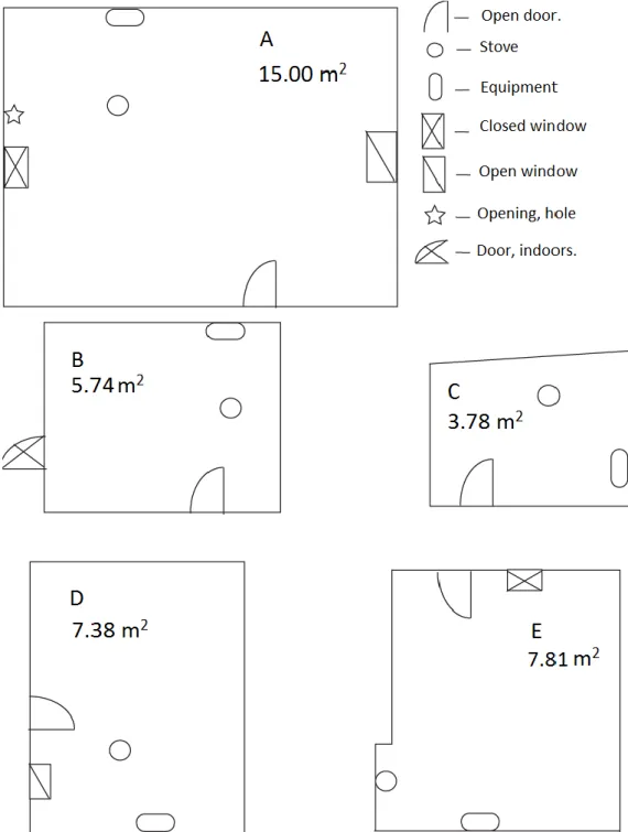
Five households were used and named in alphabetical order from Household A to Household E. The kitchens are represented in Figure 2. All kitchens were separated from the main building except for Household E that was attached to the main building. Household B had the kitchen as a part of another building and one of the doors (marked indoor in Figure 2) led to the rest of the small building. This master thesis has a different order of the households compared to the bachelor thesis from Trial 1 (Helander and Larsson, 2014). They are connected in this order (trial 2 – trial 1), Household A – C, Household B – D, Household C – A, Household D – B and Household E – E.

14

Figure 2. Schematics over the different households and they are in scale in reference to each other.

The equipment used for the experiments performed by this study:

 The temperature measurement was done with a thermometer and a thermocouple that could handle temperatures up to 1 400 ˚C. The point of the thermometer was placed between the stove and the pot, above the charcoal. The thermometer had a measurement range from -50 ˚C up to 1 300 ˚C. The accuracy was ± 0.5% rdg (reading, the temperature measured) +1 ˚C (Clas Ohlson). The thermocouple could measure up to 1 200 ˚C and the accuracy for temperatures between – 40 ˚C and 375 ˚C was ± 1.5 ˚C. For temperatures between 375 ˚C and 1 000 ˚C the accuracy was 0.004 times the measured temperature. (Jonas Bertilsson, Pentronic).

15

 A UCB particle monitor was used in this study to monitor the PM2.5 level during the cooking process. It combines ionization chamber sensing and optical scattering sensing, which a commercial smoke detector uses. It has been modified to send real-time signals, so that real-real-time monitoring and measurements can be done. When launched it had a zeroing time of at least 30 minutes, the monitor was put inside a closed zip lock bag inside a sealed airtight container. The concentration was recorded in mg/m3 _{(Household Environmental Monitoring).}

 A EL-USB-CO logger from Lascar Electronics was used to monitor the CO-level in the kitchen during the cooking process. The measurement range is between 0 and 1 000 ppm and the operating temperature is between -10 ˚C and 40 ˚C. The measurements were recorded every 10 seconds. It can store up to 32 510 measurements which is more than enough for one cooking process (Lascar).

 To measure the CO2-concentration during the cooking process a HOBO-CO2-datalogger from Onset was used. The measurement was in ppm and the device had a measurement accuracy of 50 ppm or 5 % of the measurement value (the largest value). The measurement range was between 0 and 2 500 ppm and measurements were recorded every 5 seconds (Onset).

 A kitchen scale was used to measure the fuel weight during this study. The scale had a capacity of 3 kg and the accuracy was ± 1 g (Kjell & company).

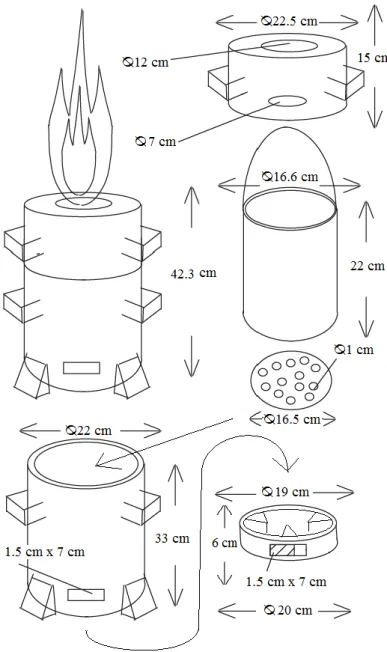
 The gasifier stove in galvanized steel was made of three different parts. The gasifier had one outer shell, a bucket for the fuel that went inside the outer shell and a top lid with one hole in the middle. See Figure 3 for the dimensions. The bucket when inside the gasifier is 5 cm above ground. The bucket was used to harvest the charred biomass.

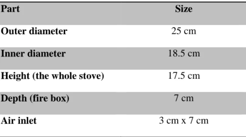
Kenya Ceramic Jiko Stove is a common charcoal stove and the one used in this study had the dimensions as described in Table 1 and was assembled as shown in Figure 4.

Table 1. Dimensions of the Kenya Ceramic Jiko stove

Part Size

Outer diameter 25 cm

Inner diameter 18.5 cm

Height (the whole stove) 17.5 cm

Depth (fire box) 7 cm

Air inlet 3 cm x 7 cm

16

Figure 3. Dimensions of the Gasifier stove.

17 3.2 Pre-cooking steps

Charred biomass was produced in the gasifier stoves in order to be able to perform the cooking tests. All the charred biomass was produced in the kitchen of one of the five households that were a part of this study to mimic the charred biomass that would be produced by the farmers if they use the gasifiers. The kitchen used for production was Household A in Figure 2. The gasifier was filled with the chosen feedstock and then lit outside of the kitchen. Dry sticks of Grevillea Robusta prunings and some dry material like leaves and branches from bushes which were to be found around the kitchen were used as lighting material. When the gasifier caught fire it was carried inside the kitchen and a pot with water was put on it to boil so to mimic the way it will be used by the farmers under normal circumstances. When the flame in the gasifier burned out the charred biomass was harvested by emptying the bucket in a pot. A lid was put on the pot to cut the oxygen supply and the pot was then put in a basin filled with water to cool. When the charred biomass cooled to room temperature it was put in a carton box for safekeeping for the tests. Three different boxes were used to store the three different types of charred biomass.

When at least one kg of one type of charred biomass had been produced, a cooking test was performed in the household where the production was done, in order to estimate how much charred biomass needed to be produced for the entire set of cooking tests. The cooking test was performed the day after production when the emissions from the production were aired out as not to affect the test.

The weight of the charred biomass/charcoal was measured with the kitchen scale. The weather and cooking conditions were recorded before each cooking test to see if any special

source of error could be found later in the results. There might have been a rainy day (higher moisture content) or some changes in the kitchen (stove moved around in the kitchen etc.). A field work sheet was produced and printed for the record keeping during the cooking process in the field. The field work sheet can be found in Appendix A1. The kitchens were prepared so that they were at the same conditions as the kitchens in the first stage of the research project (Helander and Larsson, 2014). Doors and windows were to be open and closed in accordance to Figure 2 in Section 1.4.

The bulk density was determined by filling up a container with a known volume of the

different types of fuel and weighing the container before and after it was filled. The volume of the container was 4 450 ml ± 10 ml. The measurement was done five times for each fuel type. To determine the bulk density the mean weight of each fuel type was divided by the volume of the container as in equation 3.2.1.

Bulk density = mean weight for five tests / volume of container [g]/[dm3]= [g/dm3] (3.2.1)

3.2.1 Charred biomass production from Grevillea prunings, maize cobs and coconut husks

To calculate how much charred biomass was needed per cooking test a complete cooking test was performed in Household A for each type of charred biomass. To be sure that the amounts of charred biomass per cooking test (APERCOOK) was enough it was set to the double the amount that was used during the first cooking test. When charred Grevillea prunings was used

18

the test consumed 390 g and in order to make sure that enough charred Grevillea prunings were produced the amount needed per cooking test was set to 800 g. ATESTS in eq. 3.2.1.1 was set to four tests per feedstock since there were only four households left in which to perform the cooking test. The extra charred biomass (AEXTRA) was produced so that the bulk density test could be performed and used as a backup in case that more charred biomass was needed than the estimated APERCOOKING per cooking test. AEXTRA was set to 1 kg. As equation 3.2.1.1 shows the total amount of charred Grevillea prunings needed (ATOT1) was estimated to be 4 200 g.

A TOT = APERCOOKING* ATESTS + AEXTRA (3.2.1.1)

ATOT1 = 800 * 4 + 1 000 = 4 200 g

The same procedure was used for maize cobs and the coconut husks. The difference is that for maize cobs APERCOOKING was set to 1 000 g since 449 g of charred maize cobs were used during the first cooking test. The total amount of charred maize cobs needed (ATOT2) was estimated to be 5 000g.

ATOT2 = 1 000 * 4 + 1 000 =5 000 g

For coconut husks APERCOOKING was set to 800 g since 379 g of charred coconut husks were used during the first cooking test. The total amount of charred coconut husks needed (ATOT3) was estimated to 4 200 g.

ATOT3 = 800 * 4 + 1 000 = 4 200 g

3.3 Cooking test

The cooking test was performed in five households, with three different types of charred biomass, charred Grevillea prunings, charred maize cobs and charred coconut husks and with conventional charcoal from the market in Embu used as a reference. The raw material from which the conventional charcoal was produced is unknown, but all the conventional charcoal was produced from the same raw material. A Kenya Ceramic Jiko stove was used for the cooking tests. The same households that were used in the earlier stage of this research project (Helander and Larsson, 2014), were used in this study. The time when the cooking started and finished (after the ignition of the fuel) was documented. The order in which the trials were done was randomized using Matlab’s function rand except for the tests at Household A since they were already done during the production days. Some changes had to be done to the list to match the work schedule of the farmers. See Appendix A2 for the final randomized list. During the trials the following parameters were observed:

 Time to cook a standard meal

 Amount of fuel used per cooking test

 Amount of food cooked

 If fuel had to be added during the process and if so how many times it was necessary for one meal.

19

 The flame temperature during cooking

A standard meal was defined as Ugali and Sukuma Wiki. One pot was used for cooking the Sukuma Wiki and a different pot was used for Ugali. These are traditional dishes consisting of a kind maize porridge (Ugali) and fried kale, tomatoes and onions (Sukuma Wiki). The pot for Ugali had to be changed to a thicker pot since cooking Ugali requires a thicker pot than Sukuma Wiki. For each cooking test the same amount of the ingredients were used. The amounts were 1 kg of Soko maize flour, two bags of kale from the local market always prepared in the same way (about 700 g), three tomatoes (200 g - 300 g), two red onions (80 g - 120 g) and the Sukuma Wiki was fried in coconut fat (~ 80 g).

The whole cooking process was measured from when the fuel was ignited until dish two was

finished.The time was recorded when:

 the stove was ignited (outside so no emissions were recorded from this step)

 the stove caught fire (also considered start of boiling time)

 the cold water boiled

 dish one started

 dish one finished

 dish two started

 dish two finished (considered the end of the total cooking time)

The total cooking time was the time from that the stove caught fire until dish two was

finished.

The measurement of emissions was done with the equipment hanging one and a half meter

above the ground and one meter to the side of the stove, to simulate the location of the person cooking in relation to the stove. The measurements started 30 min before the cooking started and ended 30 minutes after the cooking had ended. In the data analysis, data from the total cooking time were used. To measure the temperature the thermometer and the thermocouple were used. CO was measured with the EL-USB-CO logger, particulate matter (PM2.5) was measured with UCB particle monitor and CO2 was measured with the CO2-datalogger.

The flame temperature was measured during the whole cooking process in eight minute

intervals. The amount of fuel used was determined by weighing the pre-prepared fuel before and after the cooking process. In case of reload of fuel it would be taken from the already prepared amount of fuel which was prepared to be more than enough for cooking a meal. If adding of fuel was necessary, the time when it was added was recorded in the field work sheet.

3.4 Energy use efficiency

The energy use efficiency was determined in the unit amount of energy [kJ] used per cooking test using equation 3.4.1. The amount of energy used per cooking test was determined and the different types of charred biomass were compared to the reference charcoal from the local market. The amount of energy used per cooking test was defined in two different ways, gross fuel and net fuel. Gross fuel is when all the fuel used during the cooking test is considered to

20

be used including the amount of fuel left in the stove. The net fuel is when the fuel left in the stove is considered to have the same fuel quality as before the cooking test and then considered unused.

Energy used per cooking test [kJ /per cooking test] = Amount of fuel (g) per cooking test * calorific value * 4.1816 [g * kCal/g* J/Cal] (3.4.1) The mean energy use per cooking test was calculated for the four fuel types in the five different households using equation 3.4.2. The cooking process was assumed to be the same in the households independent of fuel used. The mean power released during cooking was calculated using equation 3.4.3. All the mean values were processed with the Kruskal-Wallis test to determine significant difference in mean between the fuels.

The mean energy use per cooking test was calculated using equation 3.4.2. The energy use for one type of fuel was summated for the five households it had been used in and divided with the number of households:

( ∑ Energy used per cooking test in household (i) ) / Total number of households (3.4.2) Where i = [1, 2, 3, 4, 5].

The mean power can be calculated as the amount of energy used per cooking test divided by the time it took to cook the meal as in formula 3.4.3:

Mean power [kJ / sec] = (∑ (Energy used per cooking test / total cooking time) ) / Total number of households (3.4.3) The amount of energy used per cooking test can be calculated with formula 3.4.1 which is the mass of the total amount of fuel used during one cooking test multiplied with the calorific value of the fuel, which were analyzed in a research laboratory (KEFRI). The method for determining the calorific value was as follows:

The sample was grinded and one gram was taken and wrapped with tissue paper of known calorific value and weight. It was then tied with an ignition wire (platinum) of known calorific value. Both ends of the wire were then connected to bomb calorimeter electrodes and then placed in a bomb calorimeter and firmly closed. Thirty kg of oxygen was then led into the bomb and the bomb immersed into a cylinder filled with distilled water up to 2 100 g. The bomb calorimeter was calibrated with benzoic acid tablets of known calorific value (see Appendix B1 for further information of how the laboratory results were obtained).

The energy density was calculated using the bulk density, conversion value from calories to joules and the calorific value obtained in the laboratory results as in equation 3.4.4.

Energy density [kJ/m3] = Bulk density * calorific value * 4.1816 [g/m3*kCal/g*J/Cal] (3.4.4) The energy balance for using the gasifier and the produced charred biomass for cooking can be calculated with equation 3.4.5.

21

The energy used per cooking test is used to cook a meal and to produce charred biomass. A mean energy use is calculated for each type of fuel and it is divided with 1+a, a = produced amount of charred biomass / charred biomass needed to cook a meal. The meal cooked with the gasifier is represented with the value 1 and a is the number of meals the produced charred biomass can cook.

3.5 Emission data analysis

The emission data collected in the field had to be processed in Excel and Matlab since each dataset for CO, CO2 and PM2.5 contained a lot of information. For PM2.5, data was recorded once a minute during the cooking period. The corresponding sampling period for CO was 10 seconds and for CO2 the sampling period was 5 seconds. The data only consisted of observations from directly after the stove was lit until the last dish was finished so the data did not include background data from before or after combustion.

The typical behaviors for the three different types of emissions were presented in graphs. The emission data for CO, CO2 and PM2.5 were processed using Matlab to plot the curves as concentration (Y-axis) versus time (X-axis) plots. To determine if there was a significant difference between the different households and the different types of fuel, an ANOVA or Kruskal-Wallis were performed. The preferable choice would be an ANOVA since it processes more information than the Kruskal-Wallis. One of the assumptions of ANOVA is that the data has to be standard normal distributed (Exploarable). One-way Kolmogorov-Smirnov test (Mathworks, kstest) and the Jarque-Bera test (Mathworks, jbtest) were used to evaluate whether the data were normal distributed. Five random measurements were chosen from each type of pollutant. Both tests showed that the data was not normal distributed. Therefore the Kruskal-Wallis test was selected as the method used to determine whether the data had a significantly different mean or not, since the ANOVA could not be applied here. The Kruskal-Wallis test rank the observations as explained in Section 2.3 and compare the mean ranks of each group against each other. If one group has a higher mean rank, then it would mean that those observations have higher values than the other groups. The Kruskal-Wallis test was done in Matlab using the function kruskalwallis.

The data for one cooking test consists of three datasets (one for each type of pollutant) with a different amount of data points depending on the type of pollutant. Each pollutant was tested on its own and not in combination with the other types of pollutants. The data was handled in three different ways before it was processed in the Kruskal-Wallis test as follows:

1. The mean value for each dataset was calculated and used as an observation, which meant that the 20 tests had 20 mean values for each emission. The mean was for the part of the dataset that corresponded to one complete cooking test (total cooking time).

2. The highest value was identified for each dataset in the interval for when the cooking test was performed resulting in 20 top values for the 20 tests for each emission. 3. The whole dataset in the interval of one complete cooking test was used as one

observation which meant that for the 20 tests there were 20 vectors of data for each pollutant.

22

For the last alternative it can be interpreted as the number of observations is equal to the number of data points, which is not correct. The purpose was to compare the dynamic of the measurements. The Kruskal-Wallis test was done in two ways, one where the different groups were divided by type of fuel (4 types of fuel with 5 observations in each group) and the other where the different groups were divided by the household number (5 groups with 4 observations in each). When the Kruskal-Wallis test was performed, the results were presented in an ANOVA-table. If the Kruskal-Wallis test showed significant difference between the groups then Matlab performed a Tukey’s HSD test to find which group was significantly different from the others. The Matlab function used is called multcompare and it uses Tukey’s HSD as a default.

The emission for charred Grevillea prunings and conventional charcoal from Trial 2 were compared to the emission from the gasifier, the improved stove and the 3-stone-fire from Trial 1 when Grevillea prunings were used. The comparison was made for the mean value and the whole dataset for each cooking test. This was done for the PM2.5-emission and the CO-emission separately.

4 Results for energy use efficiency

The results are divided into different sections as follows. The amount of fuel used for each test as well as the energy density and bulk density of the fuels are presented in Section 4.1. The energy use efficiency, the energy balance and the mean power are presented in Section 4.2. The time measurements for different steps of the cooking tests are presented in Section 4.3. A full table with the P-value for each Kruskal-Wallis test is presented in Appendix B2. 4.1 Amount of fuel used, energy density and bulk density test

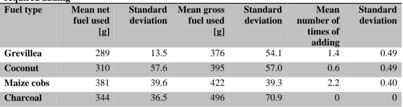
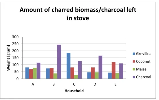
The mean mass of net fuel used and the mean use of gross fuel for each fuel type is displayed in Table 2. There is a significant difference (P=0.0201) between charred Grevillea prunings and charred maize cobs for both net and gross fuel. There are no significant differences between the other combinations of fuel types. The whole amount of fuel used during the cooking test including the fuel left in the stove is presented in the fourth column of Table 2. There are no significant differences in the mean use of gross fuel. Raw data for fuel consumption for each household and fuel type can be found in Appendix C1. Figure 5 shows the amount of fuel that was left in the stove after a completed cooking test.

Table 2. Mean use of charred biomass per cooking test and the mean number of times it required adding

Fuel type Mean net fuel used [g] Standard deviation Mean gross fuel used [g] Standard deviation Mean number of times of adding Standard deviation Grevillea 289 13.5 376 54.1 1.4 0.49 Coconut 310 57.6 395 57.0 0.6 0.49 Maize cobs 381 39.6 422 39.3 2.2 0.40 Charcoal 344 36.5 496 70.9 0 0

23

Figure 5. Amount of charred biomass or charcoal left in the stove after a completed cooking test.

The laboratory results from Kenya Forestry Research Institute Karura (KEFRI) performed by Moses Elima Lukibisi are presented in Table 3. The samples were from the different types of charred biomass and the conventional charcoal.

Table 3. Fuel properties of the different fuel types from laboratory results Sample Name MOISTURE

CONTENT % VOLATILE MATTER % ASH CONTENT % FIXED CARBON % CALORIFIC VALUE Kcal/g Maize Charcoal Cycle(2) 8.04 27.54 5.28 59.14 6.865 Coconut Shell Charcoal 5.78 19.84 4.71 69.67 7.584 Grevillea Charcoal Cycle(2) 6.73 31.84 5.15 56.28 6.342 Lump Charcoal Cycle 2 4.58 16.21 2.24 76.97 7.918

The calorific values from Table 3 are converted from calorific value [Kcal / g] to specific energy [MJ / kg] and are presented in Table 4.

0 50 100 150 200 250 300 A B C D E Wei gh t [g ram ] Household

Amount of charred biomass/charcoal left

in stove

Grevillea Coconut Maize Charcoal

24

Table 4. Specific energy for each charred biomass and charcoal [MJ/kg]

Type of fuel

Grevillea Coconut Maize Charcoal

Specific energy

26.52 31.71 28.71 33.11

The bulk density for the different types of charred biomass and conventional charcoal are presented in Table 5. The bulk density for the different fuel types were calculated by using Equation 3.2.1 in Section 3.2. The raw data for Table 5 is found in Appendix C2. The bulk density for charred maize cobs is significantly different (P=0.0007) from charred coconut husks and conventional charcoal. There are no significant differences between the other combinations of fuel types.

Table 5. Calculated bulk density for the different types of charred biomass/charcoal

Type of fuel Bulk density [g/dm3_] Standard deviation Significant difference Grevillea prunings 137.0 7.55 No Coconut 267.0 13.66 No

Maize cobs 99.10 3.34 Yes

Charcoal 277.5 15.39 No

The energy density for each fuel type is presented in Table 6, which was calculated using the calorific value from Table 3 and the bulk density from Table 5. Charred maize cobs are significantly different (P=0.0005) from charred coconut husks and conventional charcoal. Charred Grevillea prunings are also significantly different from conventional charcoal.

Table 6. Energy density based on calorific value from lab test and bulk density

Type of fuel ity [kJ/m_{Energy density [kJ/dm}3_] 3_{] Standard deviation}

Grevillea 3 630 200.0

Coconut 8 467 433.3

Maize 2 840 95.8

25

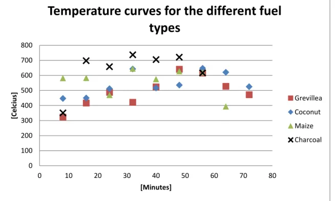
Figure 6. The temperature curves for 4 different tests, with 1 test for each fuel type.

Temperature curves representing each fuel type are presented Figure 6. Charred Grevillea prunings have a lower temperature for the most part of the cooking time and conventional charcoal has a higher temperature.

4.2 Mean energy use, mean energy balance and mean power

The mean energy consumption for cooking a meal in a Kenya ceramic Jiko stove with charred biomass produced from gasifiers is displayed in Table 7. The mean net energy use per cooking test for charred Grevillea prunings is significantly different (P=0.0298) from the corresponding value for conventional charcoal. The rest of the fuels do not have significantly different means from each other. There were no significant differences in the mean gross energy use.

Table 8 and Table 9 consist of data collected by Hanna Helander and Lovisa Larsson (Helander and Larsson, 2014). Table 8 shows how much energy was consumed to cook a meal and the yield of different types of charred biomass with the gasifier stove. There were no significant differences between the different feedstocks in terms of energy consumption,

0 100 200 300 400 500 600 700 800 0 10 20 30 40 50 60 70 80 [Ce lc iu s] [Minutes]

Temperature curves for the different fuel

types

Grevillea Coconut Maize Charcoal

Table 7. Mean net energy use per cooking test with charred biomass and charcoal Fuel type Mean net energy

use [kJ] Standard deviation Mean gross energy use [kJ] Standard deviation Grevillea 7 675 358.4 9961 1 435 Coconut 9 837 1 826 12 530 1 809 Maize 10 940 1 136 12 100 1 130 Charcoal 11 160 1 448 15 860 2 986

26

charred biomass production and amount feedstock used. Energy value is the product of the calorific value, the amount of feedstock used and the conversion value from calories to Joule.

Table 8. Mean energy consumption for producing charred biomass and cooking a meal with a gasifier stove Type of fuel Feedstock used [g] Standard deviation Charred biomass produced [g] Standard deviation Energy value [kJ] Standard deviation Grevillea 1 820 167.8 349 31.3 35 700 3 290 Coconut 1 654 330.1 390 89.0 34 700 6 920 Maize 1 514 261.8 317 61.4 28 500 4 930

The mean energy consumption between the different feedstock and the different stoves are presented in Table 9. There is a significant difference between maize cobs used in a gasifier and Grevillea used in a 3-stone-fire. Otherwise there were no significant differences between the different fuels and stoves in energy consumption. The energy consumption for gasifier stoves are in Table 9 presented with the energy value for the produced charred biomass subtracted from the total energy consumption for the gasifiers.

Table 9. Mean energy consumption per cooking test [kJ] with energy value for produced charred biomass subtracted from the gasifier tests. Type of stove Type of fuel Energy cost per meal [kJ]

3-stone-fire Grevillea 30 700

Improved stove Grevillea 24 700

Gasifier Grevillea 26 400

Gasifier Coconut 22 300

Gasifier Maize 19 400

The energy balance for using the gasifier stove in combination with the Kenya ceramic Jiko stove was between 16.3 - 18.4 MJ per meal (gross fuel, Table 10) and 15.3 MJ and 16.1 MJ per meal (net fuel, Table 11). There were no significant differences between the fuels in either the net fuel or the gross fuel case.

27

Table 10. Energy balance per meal for gross fuel

Type Mean energy consumption per meal [MJ] Standard deviation Grevillea prunings 18.4 1.74

Coconut husks 17.3 3.10

Maize cobs 16.3 2.79

Table 11. Energy balance per meal for net fuel

Type Mean energy consumption per meal [MJ] Standard deviation Grevillea prunings 16.1 1.21

Coconut husks 15.3 3.17

Maize cobs 15.5 2.66

The mean power that the stoves used is presented in Table 12, where charred Grevillea prunings have the lowest power with 1.98 kW and conventional charcoal has the highest power with 3.06 kW. The mean power with charred Grevillea prunings is significantly less (P=0.0029) than with charred maize cobs and conventional charcoal.

Table 12. Mean power during the total cooking time [kW]

Fuel type Mean power Standard deviation Grevillea 1.98 0.110

Coconut 2.48 0.541

Maize 2.82 0.340

Charcoal 3.06 0.448

4.3 Cooking time

The mean total cooking and boiling time was similar for the different types of fuel, which Table 13 shows, but between the different households the mean total cooking and boiling time was quite different, which can be seen in Table 14. However, there are no significant differences in boiling time or total cooking time between the households or the fuel types. Household B had the fastest total cooking time and Household E had the longest total cooking time.

28

Table 13. Mean boiling time and mean cooking time (incl. boiling time, Dish 1 and Dish 2) for the different fuel types [min]

Type Mean boiling time

Standard deviation

Mean cooking time Standard deviation Grevillea 19.8 2.04 66 8.2 Coconut 20.6 3.01 66 11 Maize cobs 20.0 3.74 65 2.8 Charcoal 19.2 2.93 62 6.6

Table 14. Mean boiling time and mean total cooking time for the different households [min] Household Mean boiling time Standard deviation Mean total cooking time Standard deviation A 17.8 0.829 65 7.4 B 18.8 1.48 53.8 6.67 C 22.5 3.28 62.8 4.61 D 18.8 3.11 63 4.9 E 21.8 2.28 70.8 4.84

The mean cooking times for Dish 1 and Dish 2 depending on fuel type are presented in Table 15. There are no significant differences between the different fuel types for either Dish 1 or Dish 2.

Table 15. Mean cooking time Dish 1 and Dish 2 for each fuel type [min]

Type Dish 1 Standard deviation Dish 2 Standard deviation

Grevillea 15 6.0 25 3.2

Coconut 16 8.1 25 3.4

Maize cobs 13 1.9 23 1.4

Charcoal 15 8.7 22 3.1

The mean cooking time for Dish 1 and Dish 2 are presented in Table 16. There is a significant difference (P=0.0135) between Household A and Households B and C for Dish 1. There are no significant differences between the households for Dish 2.

Table 16. Mean cooking time Dish 1 and Dish 2 for each household [min]

Household Dish 1 Standard deviation Dish 2 Standard deviation A 25.3 6.6 22 2.2 B 9 2 23 3.0 C 10.3 0.83 22 2.2 D 14.3 3.27 27 1.9 E 15.3 3.27 26 2.6

29

5 Emission results for Trial 2

The emission for the different types of charred biomass (Trial 2) has been evaluated and compared to each other. This section has been divided into two different subsections for each type of pollutant except for CO2-emissions and one subsection for comparison with Trial 1. The data from the CO2-measurements could not be analyzed properly, due to a lack of data since two measurements failed for the CO2-emission because of technical difficulties with the equipment. Figure 7 shows five tests chosen at random and the CO2-concentration during these tests. The levels varied between ~350 ppm and ~800 ppm.

Figure 7. CO2-emission curves for five cooking tests chosen at random. 1 step in the x-axis represents 5 seconds.

5.1 PM2.5-emission data

The Kruskal-Wallis test was performed on the mean value, top value and the whole data set for the emission to determine if there were any significant differences. The PM2.5-emissions curves for five different tests (chosen at random) are presented in Figure 8. The mean emission level throughout the cooking time over all tests for PM2.5 is 76.3 μg/m3.

0 500 1000 1500 2000 2500 3000 3500 4000 4500 5000 300 400 500 600 700 800 900

CO2-emisson for 5 tests chosen at random

Total cooking time [Seconds]

C O 2 -c o n c e n tr a ti o n [ p p m ]

30

Figure 8. PM2.5-emission curves for five cooking tests chosen at random. The Y-axis shows the PM2.5-concentration

levels in the kitchens during cooking. The X-axis shows the total cooking time [Minutes] from when the combustion began until Dish 2 was finished.

5.1.1 Comparison of the mean value of PM2.5-emission for each cooking test

The mean value for all the PM2.5-measurements done under one cooking test (the whole cooking time) was calculated for all 20 cooking tests. The mean values for each fuel type is presented in Figure 9. A significant difference was found between the different fuel types (P=0.034) which can be seen in Appendix B2, but the post-hoc (Tukey’s HSD) could not find which one. Maize has the highest mean, but also has a large variance (Figure 10).

0 10 20 30 40 50 60 70 80 0 0.2 0.4 0.6 0.8 1 1.2 1.4

PM2.5-emisson for 5 tests chosen at random

Total cooking time [Minutes]

P M 2 .5 -c o n c e n tr a ti o n [ m g /m 3]

31

Figure 9. Mean ranks for the different types of fuel, each observation corresponds to the mean value of one household. Observation 1, 2, 3, 4 and 5 corresponds to household A, B, C, D, and E in that order.

Figure 10. A box plot showing the median for each fuel (in red), the 25th and 75th percentiles (in blue) and max and min value (in black).

1 2 3 4 5 0 0.05 0.1 0.15 0.2 Grevillea Household P M 2 .5 -c o n c e n tr a ti o n [ m g /m 3 ] 1 2 3 4 5 0 0.02 0.04 0.06 0.08 Coconut Household P M 2 .5 -c o n c e n tr a ti o n [ m g /m 3 ] 1 2 3 4 5 0 0.1 0.2 0.3 0.4 Maize Household P M 2 .5 -c o n c e n tr a ti o n [ m g /m 3] 1 2 3 4 5 0 0.02 0.04 0.06 Charcoal Household P M 2 .5 -c o n c e n tr a ti o n [ m g /m 3 ] 1 2 3 4 0 0.05 0.1 0.15 0.2 0.25 0.3 0.35

Grevillea Coconut husks Maize cobs Charcoal

P M 2 .5 -c o n c e n tr a ti o n [ m g /m 3 ] Median PM2.5-concentration

32

There were no significant differences between the households, but charred maize cobs have the highest value in each household. The mean values for the households are presented in Figure 11.

Figure 11.Mean ranks for each household with observation 1 representing charred Grevillea prunings, observation 2 represents charred coconut husks, observation 3 represents charred maize cobs and observation 4 represents conventional charcoal.

5.1.2 Comparison of the top value of PM2.5-emission for each cooking test

There are no significant differences between the fuel types or the households in terms of top values (data in Appendix B2). The top values for the different fuel types are presented in Figure 12 and for the different households in Figure 13.

1 2 3 4 0 0.05 Household A Fuel types P M 2 .5 -c o n c e n tr a ti o n [m g /m 3] 1 2 3 4 0 0.2 0.4 Household B Fuel types P M 2 .5 -c o n c e n tr a ti o n [m g /m 3 ] 1 2 3 4 0 0.1 0.2 Household C Fuel types P M 2 .5 -c o n c e n tr a ti o n [m g /m 3] 1 2 3 4 0 0.2 0.4 Household D Fuel types P M 2 .5 -c o n c e n tr a ti o n [m g /m 3 ] 1 2 3 4 0 0.05 0.1 Household E Fuel types P M 2 .5 -c o n c e n tr a ti o n [m g /m 3]

33

Figure 12.Top values for the different types of fuel. Observation 1, 2, 3, 4 and 5 corresponds to Household A, B, C, D, and E in that order.

Figure 13.Top value for each household where observation 1 represents charred Grevillea prunings, observation 2 represents charred coconut husks, observation 3 represents charred maize cobs and observation 4 represents conventional charcoal. 1 2 3 4 5 0 2 4 6 Grevillea Household P M 2 .5 -c o n c e n tr a ti o n [ m g /m 3 ] 1 2 3 4 5 0 0.5 1 Coconut Household P M 2 .5 -c o n c e n tr a ti o n [ m g /m 3] 1 2 3 4 5 0 0.5 1 1.5 Maize Household P M 2 .5 -c o n c e n tr a ti o n [ m g /m 3] 1 2 3 4 5 0 0.2 0.4 0.6 0.8 Charcoal Household P M 2 .5 -c o n c e n tr a ti o n [ m g /m 3] 1 2 3 4 0 0.5 Household A Fuel types P M 2 .5 -c o n c e n tr a ti o n [m g /m 3] 1 2 3 4 0 1 2 Household B Fuel types P M 2 .5 -c o n c e n tr a ti o n [m g /m 3 ] 1 2 3 4 0 1 2 Household C Fuel types P M 2 .5 -c o n c e n tr a ti o n [m g /m 3 ] 1 2 3 4 0 5 10 Household D Fuel types P M 2 .5 -c o n c e n tr a ti o n [m g /m 3] 1 2 3 4 0 0.5 1 Household E Fuel types P M 2 .5 -c o n c e n tr a ti o n [m g /m 3]

34

5.1.3 Comparison of the complete dataset for PM2.5-emission for each cooking test

Figure 14 shows how the PM2.5-concentration varies during the five tests for each fuel type. There is a clear significant difference between different fuel types in terms of mean rank for all the measurements taken during the cooking tests. Charred maize cobs high values differ the most from the other fuel types (see Figure 15) and charred Grevillea prunings also differ from the other fuel types. Charred coconut husks and conventional charcoal do not differ significantly from each other and have the lowest values of the different fuel types. In Figure 15 the X-axis is the rank value and this value gives no indication on its own if the value is high or low. It is only in comparison to the other rank values that one can see if the value is high or low since the rank value depends on how many measurements has been done. For a 100 data points the rank will be between 0 and 100, but for a 1 000 data points they will be ranked between 0 and 1 000.

Figure 14. Observations for the different types of fuel with five emission curves following each other with the emission curve of Household A first and in alphabetical order until the emission curve for Household E.

100 200 300 0.2 0.4 0.6 0.8 1 Grevillea

Total cooking time [Minutes]

P M 2 .5 -c o n c e n tr a ti o n [m g /m 3] 0 200 400 0 0.5 1 Coconut

Total cooking time [Minutes]

P M 2 .5 -c o n c e n tr a ti o n [m g /m 3 ] 100 200 300 400 0.2 0.4 0.6 0.8 1 Maize

Total cooking time [Minutes]

P M 2 .5 -c o n c e n tr a ti o n [m g /m 3] 0 200 400 0 0.2 0.4 0.6 0.8 Charcoal

Total cooking time [Minutes]

P M 2 .5 -c o n c e n tr a ti o n [m g /m 3 ]