Partitioning a set of functions into correlated subsets

Partitioning a set of functions

into correlated subsets

<

t:

3

I Pmar Heggernes and Pontus Matstoms

E

_e

S

Swedish National Road and

VTl rapport 416A - 1998

Partitioning a set

of functions into

correlated subsets

Pinar Heggernes

Pontus Matstoms

Swedish National Road and

Utgivare: Publikation:

VTI Rapport 416A

Utgivningsar: Projektnummer:

1 998 50014

Véig- och

transport-'farskningsinstitutet

581 95 Linkb ping Projektnamn:

Hushallens transporter

Forfattare: Uppdragsgivare:

Pinar Heggernes, Universitetet i Bergen, Norge Kommunikationsforskningsberedningen Pontus Matstoms, Statens v'ag- och transportforsknings- (KFB)

institut (VTI), Linko'ping

Titel:

Uppdelning av en funktionsm'angd i korrelerade delmangder

Referat (bakgrund, syfte, metod, resultat) max 200 0rd:

Losning av trafiktillordningsproblem (eng traffic assignment) bygger bland annat pa kanda samband mellan trafik ode och medelhastighet. I verkliga till'ampningar ferekommer era olika vagtyper med sinsemellan olika ede/hastighet samband. I ett av standardprogrammen for losning av detta problem, Emme/Z, finns en ovre grans fer det totala antalet operatorer i funktionsdatabasen. Vi foreslar en metod for att reducera antalet funktioner som maste sparas i databasen och darigenom minska antalet operato-rer. Utseendet pa de olika funktionerna ar ofta likartade, vilket gor det mojligt att begr'ansa databasen till en delm'angd av de ursprungliga funktionerna och rekonstruera 6vriga funktioner fran dessa.

Det hela kan formuleras som ett grafteoretiskt problem med en graf bestaende av noder som svarar mot funktioner och lankar svarande mot korrelationen mellan olika funktioner. Noderna i grafen delas upp i ett antal delmangder sa att noder/funktioner i samma delmangd 'ar hogt korrelerade till varandra. For varje delm'angd utses en basfunktion som, genom en linj'ar transformation, kan rekonstruera ovriga funktioner i delm'angden. Problemet kan formellt formuleras folj ande s'a'tt: dela upp funktionsmangden i ett minimalt antal delm'angder sa att funktioner i samma delm'angd, enligt ett valt kriterium, ar v'al korrelerade med varandra. Det foljer att motsvarande grafproblem kan losas fristaende fran det rent statistiska problemet. I rapporten diskuteras flera olika metoder for uppdelning av funktionerna i del-m'angder och for val av basfunktioner. De olika metoderna jamers utifran den ursprungliga trafiktill-lampningen.

ISSN: Sprak: Antal sidor:

Publisher: Publication:

VTI Rapport 416A

Published: Project code:

1998 50014

Swedish National Roadand ' anspart Research Institute

8-581 95 Linkoping Sweden Project:

Private transports

Author: Sponsor:

Pinar Heggernes, University of Bergen, Norway Swedish Transport and Communications Pontus Matstoms, Statens vag- och transport Research Board (KFB)

forskningsinstit (VTI), Link'oping, Sweden

Title:

Partitioning a set of functions into correlated subsets

Abstract (background, aims, methods, results) max 200 words:

The solution of the traffic assignment problem is based on the known ow/speed relations defined for the given network links. In real applications, there are many different road types, each with its own ow/speed function. One of the standard computer programs for the solution of this problem, Emme/Z, has an upper bound on the total number of operators that can be used in the database of ow/speed func tions. We propose a method to reduce the actual number of functions needed to be stored in the database. The forms of the functions are typically similar, and thus we can store a subset of the functions, and use these to compute the rest of the functions. This requires the solution of a statistical problem related to linear and non linear regression. Correlation coefficients between each pair of functions must be computed to see how well theycan be expressed in terms of each other.

Given the background explained above, we pose a graph problem based on the relation between the functions, with each node of the graph representing a function, and the graph edges representing the correlation between the functions. The problem of reducing the number of functions needed to be stored is reformulated as a graph partitioning problem. The nodes of the graph are partitioned into a smaller number of subsets, where the functions corresponding to nodes within a subset are highly correlated. A

base function is chosen from each subset, and only these base functions are stored in the database. Thus

the objective of the graph partitioning problem is to minimize the number of resulting subsets of nodes, where the nodes in each subset are related to each other according to some user defined criteria. Conse quently, the graph partitioning problem can be presented and solved independently of the underlying statistical problem and traffic application, and standard graph theoretical algorithms and techniques can be used as a part of the solution methods. We propose several methods both for partitioning the graph, and for choosing a base function from each subset. Numerical test results, showing how well the methods perform and comparing them, are given on the underlying application.

ISSN: Language: No. of pages:

Preface

We would like to thank Professor Alex Pothen, Old Dominion University, Mats Wiklund, VTI, and Professor Stig Danielsson, Link'oping University, for discus sions and useful suggestions. We also thank Professors Bengt Aspvall and Petter Bjorstad, and the University of Bergen for making the authors Bergen meeting possible.

Contents

Summary

Sammanfattning

Introduction

Correlated functions

Graph theoretical background

Graph partitioning methods for finding correlated subsets

Choosing base functions

Numerical examples and results

Concluding remarks

11

13

17

19

21

27

31

35

36

Partitioning a set of functions into correlated subsets by Pinar Heggernes, University of Bergen, Norway

and Pontus Matstoms, Swedish Road and Transport Research Institute, Linkoping, Sweden

Summary

With fewer functions one can retain circumstantiality of traffc

planning

A method has been developed for reducing the number of functions stored

in a database, while still allowing a detailed description of the speed

relations of the various road types. The whole set of functions is partitioned in such a way that functions of similar form appear in the same subset. A base function, representing the subset, is used to reconstruct the rest of

the functions in the same subset. Only the base functions are needed to be

stored in the database.

In this paper, we consider a statistical problem related to curve fitting and non linear models. For the solution of this problem we use graph theoretical methods and algorithms. The statistical problem we focus on arises from the set of ow/speed functions in a traffic assignment problem. In transport engineering, the relation between traffic ow and mean speed plays an important role. The mean speed is dependent on the traffic flow and this effect must be taken into account for a realistic solution of the traffic assignment problem.

The solution of the traffic assignment problem is based on the known ow/speed relations defined for the given network links. In real applications, there are many different road types, each with its own ow/speed function. One of the standard computer programs for the solution of this problem, Emme/Z, has an upper bound on the total number of operators that can be used in the database of ow/speed functions. This restriction limits the possible size of the individual functions and may be a serious problem to handle.

We propose a method to reduce the actual number of functions needed to be stored in the database. This approach allows the functions stored in the database to be described in detail without reducing the size, exibility and possible complex-ity of the individual functions. The forms of the functions are typically similar, and thus we can store a subset of the functions, and use these to compute the rest of the functions. This requires the solution of a statistical problem related to linear and nonlinear regression. Correlation coefficients between each pair of functions must be computed to see how well they can be expressed in terms of each other. Then we want to group the functions that are highly correlated into subsets and let one function from each subset represent the rest of the functions in the same subset. This way, only one function from each subset needs to be stored in the database. Clearly, we want to store as few functions as possible in the database, which is equivalent to partitioning the original set of functions into as few subsets as possible. Of course, this objective is often in con ict with the goal of each subset consisting of functions as highly correlated as possible.

Given the background explained above, we pose a graph problem based on the relation between the functions, with each node of the graph representing a function, and the graph edges representing the correlation between the functions. The problem of reducing the number of functions needed to be stored is reformu lated as a graph partitioning problem. The nodes of the graph are partitioned into a smaller number of subgraphs, where the functions corresponding to nodes within a subgraph are highly correlated. In order to solve this partitioning problem two methods are proposed. The above mentioned minimization problem corresponds to a computationally intractable graph problem. Therefore our proposed methods are heuristics, which means that the produced result is not necessarily the theo-retical optimal solution, but it gives good practical partitions that are useful for the underlying application. Our numerical tests show that functions that are grouped together actually correspond to similar road types for our test problem.

It should be stressed though that the resulting graph partitioning problem is an interesting graph theoretical problem in its own right. The methods proposed in the paper are general in the sense that they can be applied on general graphs or graphs representing other sets of related elements. It is the authors intention to describe the problem in an as general setting as possible, although the underlying problem is used to test the proposed methods.

After the partitioning is complete, a member from each subset is to be chosen to represent the other functions of the subset in the database. The choice of repre-senting function, calledbase function, from a subset is important to minimize the error when a function is computed from its corresponding base function stored in the database. We propose several methods based on graph theory in order to choose good base functions.

With the methods prOposed both for partitioning and for choosing base func tions, our numericaltests show that we achieve very good results with respect to reducing the number of functions without introducing significant errors. For the practical application described in the paper, we are able to reduce the number of functions to fit the limitations of the database, and the complete set of functions can be restored from the base functions with acceptable errors.

Uppdelning av en funktionsmangd i korrelerade delmangder

av Pinar Heggernes, Universitetet i Bergen, Norge

Pontus Matstoms, Statens vag och transportforskningsinstitut (VTI), Linkoping

Sammanfattning

Farre funktioner

bibehallen detaljeringsgrad for

trafikplane-ring

En metod har utvecklats for att reducera antalet funktioner som méste lagras i en databas utan att ge avkall pa detaljeringsgraden i beskrivningen av olika va'gtypers hastighetssamband. Hela mangden av funktioner

grupperas sa att funktioner med liknande form hamnar i samma grupp. En

representerande basfunktion kan rekonstruera 6vriga funktioner i gruppen.

l databasen behéver man da bara lagra de olika basfunktionerna.

Vid trafikplanering 'ar det ofta viktigt att, under olika foruts'attningar, kunna uppskatta trafik odet pa enskilda v'aglankar. Det gors genom losning av det sa kallade trafiktillordningsproblemet (TAP), varvid man utgaende fran hur manga som reser mellan olika platser ber'aknar forvantade vagval och resulterande trafik

o'den. Speciellt i t atortstrafik kan trangsel gora att flera olika vagval kan vara intressanta. Denna effekt fangas upp av givna samband mellan trafik ode och medelhastighet for olika typer av vagar. Typiskt minskar medelhastigheten vid Okande o'de, vilket gOr att trafiken fordelar Sig pa alternativa vagar pa ett sadant satt att restiden minimeras. Det ar ocksa under ett sadant antagande som TAP typiskt loses. I verkliga tillampningar bestar trafikn'atverket av manga olika vag typer med sinsemellan olika hastighetssamband. I Emme/Z, som ar ett standard program f6r losning av TAP, finns det fer narvarande en begr'ansning som gOr att hela mangden av hastighetsfunktioner inte far innehalla mer 'an ett visst antal operatorer. Denna begransning gor att antalet funktioner eller dess komplexitet maste hallas nere.

I rapporten fereslar Vi en metod for att reducera antalet funktioner som maste lagras utan att ge avkall pa detaljeringsgraden i beskrivningen av olika vagtypers hastighetssamband. Idén bygger pa att de olika hastighetsfunktionernas form ofta ar snarlik men att skalningen i X- och y-led varierar. Avsikten 'ar att gruppera hela mangden av funktioner sa att funktioner med liknande form hamnar i samma grupp. Fran varje grupp utses sedan en representerande basfunktion som genom olika linj'ara transformationer kan rekonstruera ovriga funktioner i gruppen. I databasen behover man da bara lagra de olika basfunktionerna. Eftersom rekonstruktion sker genom linjara transformationer 'ar den vanliga korrelations koeffieienten ett lampligt matt pa hur n ara olika funktioner ligger varandra.

Med ovanstaende bakgrund kan vi naturligt formulera problemet som ett graf-teoretiskt problem. Vi betraktar en graf med noder som svarar mot de olika funk-tionerna och bagar som svarar mot korrelationen mellan parvisa funktioner. Problemet att reducera antalet funktioner formuleras som ett grafpartitionerings problem, dar noderna delas upp i delmangder inom vilka samtliga noder 'ar parvis hOgt korrelerade med varandra. Att finna den, i nagon mening, basta losningen ar ber'akningsm'assigt besv'arligt varfér approximativa metoder bor tillgripas. Vi

foreléir tvé l olika heuristiska metoder som i praktiken Visar Sig ge bra losningar. Numeriska experiment Visar att funktioner som grupperas tillsammans svarar mot liknande V'agtyper.

Det skall understrykas att det resulterande grafpartitioneringsproblemet i Sig éir ett intressant grafteorietiskt problem. De metoder som presenteras i rapporten éir generella i den meningen att de kan till'ampas p51 allm'einna grafer eller grafer som representerar andra méingder av relaterade element. I rapporten presenteras prob lemet sé generellt som mojligt med den beskrivna trafiktilléimpningen bara som en illustration och exempel p51 tilléimpning.

Givet uppdelningen av funktioner i delm'eingder terstéir problemet att finna, representerande basfunktioner. Det éir h'ar Viktigt att V'zilja en funktion som 55 Val som mojligt kan terskapa samtliga ovriga funktioner i delméingden. Exakt Vilket kriterium som skall V'eiljas r inte sj'zilvklart utan det kan vara rimligt att overvéiga era olika mé llfunktioner. En sé tdan éir att gora det storsta rekonstruktionsfelet i delm'eingden séi litet som mojligt. Vi foresléir och jéimfor era olika metoder, samt-liga baserade p51 grafteori.

Genom numeriska experiment och j'zimforelser av de frireslagna metoderna for att gruppering och for att utse basfunktioner Visar Vi att en p taglig reduktion i antal funktioner som behover lagras kan stadkommas utan att néigot avgorande fel samtidigt introduceras. I den beskriva praktiska tilléimpningen kan antalet funktioner minskas till en tilléiten nivéi samtidigt som bara mindre avvikelser fng fréin de ursprungliga funktionerna.

1

Introduction

Mathematical and statistical modelling often include data analysis, where an observed or measured variable y is described by a set of explanation variables {Xi}. In statistics this is referred as regression analysis, while the terms curve fitting and approximation are used in mathematical modelling and engineering. The purpose is usually understanding the mechanism behind the observed variation in y, separating the real variation in y from random errors, interpola-tion, and extrapolation (forecasts). Often the object is simply to get an analytic expression for y that approximates the observed variation in data.

In many cases, the most natural approach is to use linear regression where y is

expressed as a linear function in the explanation variables,

A n

yZCO +Zi=1ci 'x "

Although other approaches exist, the unknown coefficients c,- are generally determined by the least squares method, making the Euclidean norm of the residual vector r = 9 )2 minimal,

- 2

min 2 n ._C

The linear model is naturally formulated in terms of matrices and solved by methods based on concepts in linear algebra. If the model is written as the over determined linear system szb, the least squares formulation is given by

minlle bllz,

X

and solved by a standard method like the normal equations, ATAx = ATb, or by

QR factorization of the matrix A [Bjorck (1995)].

In many applications, however, linear models are insufficient and more general non-linear functions must be considered, for example polynomials or exponential functions. The same solution technique as in the linear case can then sometimes be used, either

directly or after a mathematical transformation of the model. Otherwise, in the most

general case, the computationally more expensive non-linear least squares problem has to

be solved [Dennis (1977)].

In this paper, we consider a statistical problem related to curve fitting and nonlinear models as described above. For the solution of this problem, we will use graph theoretical methods and algorithms. Although the problem is described in terms of a particular application, it is of general relevance in its own right. Especially, the graph theoretical issues and questions that arise are of interest independently of the underlying problem. We will state our main problem as a graph partitioning problem whose solution is based on general algorithmic techniques. However, we feel that the discussion gains in clarity by presenting the underlying problem in terms of its practical background.

In transport engineering, the relation between traffic ow and mean speed plays an important role. One example is in the solution of the tra ic assignment

origin/destination (OD) matrix describing the number of trips between all

combinations of nodes, the traffic assignment solution estimates the traffic flow

on the individual network links. "

If the mean speed on the links were constant and independent of the traffic flow, then the traffic assignment problem could be replaced by the all pairs shortest path problem. Assuming that drivers take the shortest path (in time), the ow on a certain link could be estimated simply by counting the number of vehicles travelling on all paths including the considered link.

Now, the mean speed is indeed dependent on the traffic ow and this effect must be taken into account for a realistic solution of the traffic assignment problem. This leads to an iterative procedure, consisting of repeated updates of the shortest path solution according to the known ow/speed relations. It is in particular important to capture the typical decrease in speed as the ow increases and reaches a congestive level. At this point, or earlier, drivers are supposed to consider alternative routes and distribute themselves in the network according to Wardrop s principle [Sheffi (1985)]: " '

Under equilibrium conditions tra ic arranges itself in congested networks such that all used routes between an 0-D pair have equal and minimum costs while unused routes have greater or equal costs.

In a real traffic network there are different road types with different speed limits and number of lanes. Each type has its own ow/speed relation. From empirical data, functions of the general form

c3-Q

v(Q) = c0 +

1+c4-e

are generated to describe the relation between traffic flow Q and mean speed 120 on different roads types [Matstoms et al. (1996)]. Here, ci,i =0,...,4, are the

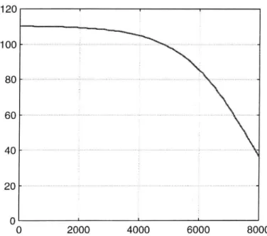
unknown coefficients determined by the least squares method. In our particular application we have 61 road types and for each of them a unique ow/speed relation. A typical speed function is shown in Figure 1.

Many computer programs for the solution of the traffic assignment problem

are available today. Emme/2 [INRO (1991)] is one of the most well known, and it

is considered in the application described here. Besides a detailed description of the network, the input data also includes a set of ow/speed functions and, for each link, a reference to an appropriate function from this set.

In Emme/2 there is an upper bound for the total number of operators1 that can be used in the database of ow/speed functions. This restriction limits the possible size of the individual functions and may be a serious problem to handle. If, for example, the functions should model the link speed as well as junction delays, then the operator limit is easily exceeded.

Instead of reducing the size, exibility, and possible complexity of the individual functions, we propose a method to reduce the actual number of functions that need to be stored in the database.

1 In Emme/2 operators include, for example, +, -, *, /, ex, logical operators and min/max.

120 100 80 60

4o

Figure I The ow/speed relation for one of the considered road types (4 lane highway with speed limit 110 km/h). Here, the x axis is the tra ic ow

(vehicles/h) and the y-axis the mean speed (km/h).

Let us consider the original set of ow/speed functions (Q),i =1,...,N. Since the general form of the various functions are similar, but the level and scale of the ow varies, it is reasonable to believe that storing a small subset of the functions should be enough, and that the remaining functions can be reconstructed by a simple transformation of one of the stored base functions. Thus, our idea is to

select a small set of base functions bl.(Q),i = l,...,n, from the original set and then

be able to, with tolerable error, express any of the other original functions by a linear transformation of a base function:

HQ) = a ) + ,8 ) 42,. (Q).

Hence the problem considered in this paper can be stated as follows:

1. Partition the original set of functions { } into a smaller number of subsets of

closely related functions.

2. For each subset, choose one base function, such that the other functions in the subset can be removed and reconstructed from the base function.

To implement this idea in Emme/2, for each original function we need to store

the associated coefficients a and ,8, and a reference to the related base functionz.

To evaluate one of the original functions, the base functions are modified such

that the above linear transformation is included. The above mentioned partitioning problem is formulated as a graph partitioning problem in Section 4, and solution methods are suggested and discussed.

2 In Emme/2 this is implemented as user data or as data table.

The outline of the paper is as follows. In Section 2, we give a theoretical background and a more detailed description of the problem. As mentioned, the methods discussed throughout the paper are derived using concepts from graph theory, and thus a short introduction with the necessary definitions is given in Section 3. In Section 4, we propose a method for partitioning the original set of functions into correlated subsets. The problem of selecting the best base function of each subset is discussed in Section 5. In Section 6 we illustrate the results by numerical examples related to the traffic application. Throughout the paper we use the macro language of Morlob [MathWorks (1992)] to define proposed methods. Finally, some concluding remarks are given in Section 7.

2

Correlated functions

Two stochastic variables, x and y, are said to be perfectly correlated if one of them can be expressed exactly as a linear function in the other,

y=a+ x.

In practice, however, this is not often the case. Instead, errors in

measure-ments and the fact that an exact model also may include non-linear components, often make the linear model sufficient but not perfect. In this case there is indeed

a difference between the model and observed data, but the residual is relatively small and the model still relevant.

A useful measure of the linear association between the two variables is the absolute value of the correlation coefficient

C0v(x, y) I VlVarOC) - Var(y)' .

px,y :

IIere,

C0v(x, y) = E((x #1 )(y #2 l)

is the covariance of x andy, and E() and VarO denote the expectation and

variance, respectively, and ,u1=E(x) and ,u2=E(y). It can be shown that correlation coefficients lie between 1 and 1. For our purposes the sign is not relevant, and in the following we will refer to pm, as the correlation coefficient. If pm =1 then x and y are perfectly correlated, and if pm, =0 then the variables are said to be uncorrelated and linearly unassociated. In the latter case it should, however, be noticed that x andy still might be statistically dependent but notfollowing a linear model.

It should be pointed out that the correlation coefficient in it self does not tell everything we need to know. It is easy to find examples of two pairs of vectors (x,y) and (u,v) where the correlation coefficients pm, and pw, respectively, are about the same but error in linear approximation differs considerably. Thus, a correlation coefficient close to unity does not guarantee a small model error. This effect is explained by the following result.

Let (x, y) be a pair of vectors with the correlation coefficient pm, and let y=a+ ,Bx be the best linear least squares estimator of y. Then it can be shown that the variance of the model error is given by

varo r) = 030 p3,.)

where O'y denotes the standard deviation of y. It follows that the correlation

coefficient as well as the standard deviation of y are important for a small model error.

Let us now return to the problem described in the introduction. Given the set of original functions fl.(Q),i =1,...,N, we are looking for a partition into n < N

subsets such that all functions in a certain subset, with acceptable accuracy, can be expressed by a linear transformation of the base function for that particular subset. The problem can be reformulated in terms of the following two subproblems:

1. Find an optimal partitioning of the original set of functions.

For each subset, choose the best function to represent the other functions in that subset.

Here, by an optimal partitioning, we mean a minimum number of subsets where all the functions in each subset are highly correlated. In Section 4, we give

a more formal definition of Problem 1. It should be noted, though, that the optimal

solution might be time consuming to find for the general case, and hence we concentrate on finding good (not necessarily optimal) partitions.

Let pm denote the correlation between functions - and . This value and all

other quantitative measures are from now on based on numerical evaluation of the functions for discrete values of Q on the considered interval. The particular choice of discretization may indeed have some in uence on the results. By non-uniform discretization it is possible to focus on particular subintervals, for example intervals containing rapid changes of the curve. However, throughout this paper we use uniformly distributed values of Q with step length Q,- -Ql-_1 =10. It turns out that the exact choice of step length is not critical.

Subproblem 1 can be seen as a clustering problem, where we under the distance measure 1 pin]. partition the original set of functions in such a way that functions close to each other are grouped together. Extensive research has been done on cluster analysis, and a comparison of frequently used methods is given by Gower in [Gower (1967)]. In our paper we propose a different approach based on graph theory.

The following discussion and some of the described methods are based on a

matrix R of correlation coefficient, where the rows and the columns of R

correspond to functions in the given function set S.

(1 101,2 101,3 p],N \ 1 102,3 p2,N R: " " 3

1 ION LN

\

1 /

This matrix is symmetric and therefore we only need to compute and store the upper triangular part. In addition, since the diagonal is obviously l for all cases, it is sufficient to store the strictly upper triangular part of R (zero diagonal).

In our approach to solve the partitioning problem, the functions are grouped together according to a user defined bound T on the correlation coefficients. Thus pairs of functions that have a higher correlation coefficient than T are considered to be highly correlated, and the partitioning is based on 2'.

3

Graph theoretical background

In this section, we introduce the necessary graph theoretical background and terminology for expressing the problem mentioned in the previous section as a graph problem.

A graph G = (V,E) consists of a set V of nodes (also called vertices), and a

set E of edges, where E g {(a,v) l a,ve V}. We consider undirected graphs with no self loops, which means that (u,v) is the same as (v,a), and u at v for each pair (a,v)e E . If (Ll,V) is an edge in G, then u and v are called neighbors. The degree

of a node is the number of its neighbors. A graph is complete if all pairs of nodes are neighbors, or equivalently, if all vertices have degree IV I 1.

A path between a node a and a node v is a sequence of nodes [u,w1,w2,...,wk,v] that are connected by the edges (a, w1 ),(w1 , wz),...,(wk , v). A node a is said to be reachable from a node v if there is a path between v and u. A graph is connected if there is a path between every pair of nodes in the graph.

A subgraph of a grath = (V,E) is a graph H =(U,F) such that U g V, and F g E . A clique is a complete subgraph. A clique is maximal if it is not contained in any other clique. If a graph G is not connected then it can be partitioned in a unique way into a set of connected subgraphs called the connected components of G. A connected component of G is a maximal connected subgraph of G.

Listing the nodes in a graph, or visiting each node once in a certain order, is called traversing, or searching, the graph. There are several standard and well-known algorithms for graph traversal. One of these, which is suitable for our purposes, is depth-first search. The idea behind this search method is to follow a path as far as we can until we encounter nodes that are already visited. The search starts at a node v which is marked visited immediately, and follows a path continuing from v through one of its unmarked neighbors as far possible without visiting any node more than once. Each node is marked visited as they are traversed. When a path cannot be followed further, we backtrack along the path and continue with an unmarked neighbor of the latest node on the path that has such a neighbor. This can be achieved easily with the following recursive algo-rithm:

dfs(G,v) mark V

for all edges (v,w) do

if w is unmarked then

dfs(G,w)

end if

end for

Lemma: If G is connected, then all the nodes in G will be marked after a traversal with dfs (G, v), for an arbitrary node v in G.

Proof: Assume on the contrary that G is connected and that there is a set U of unmarked nodes after a traversal with dfs (G, v) . Since G is connected, there must be at least one node u in U that has a marked neighbor. But this leads to a

diction since all neighbors of a marked node are also visited and marked by the algorithm.

If G is not connected, then the connected components of G can be found by

depth-first search. A depth-first search starting from a node v will mark all the nodes in the same connected component as v. If there are unmarked nodes left

after this traversal, then by the above lemma, these must belong to other

connected components. The depth-first search can be repeated as long as there are unmarked nodes in the graph. D

4

Graph partitioning methods for finding

corre-lated subsets

In order to introduce and explain the idea of representing a set of functions and the relationship between them as a graph, let us first assume that we have a set S of N functions, where some of the functions can be expressed exactly in terms of other functions in the same set, in other words, some pairs of functions are perfectly correlated. In the case where a function can be expressed in terms of another function, we do not want to keep both the functions, but just one of them. Let f] Efg denote that functions f; and f2 are perfectly correlated. Obviously, the E is a symmetric and transitive relation. Iff; Efz, then f2 5f] inversely. IffIEf2 and f2 57% then f] sf3, and we need only one of the functions f1, f2, and f3 to be able to express them all. The functions in S can be arranged in a matrix R showing the symmetric and transitive relationship between them. Then R is an NX N symmetric matrix where the rows and the columns represent the functions, and where Rid-=1 if 12- E , and Ri,j=0 otherwise. Such a matrix can be interpreted as a

graph G(R) =(V,E) where V = {1,...,N}, and (i,j)e E if and only if Rid-=1.

Lemma: G(R) is either a complete graph, or it consists of connected components that are cliques.

Proof: Assume that G(R) has a component C that is not a clique. Then there must

exist two vertices i and j in C where (i, j) is not an edge in G(R). By definition of

connected components, there must be a path between i and j in C, [i, k], k2,...,km, j]. But then, by transitivity of 5, (i, j) should also be an edge of G(R), which

leads to a contradiction. D

Now, each connected component C of G(R) is a maximal clique and defines an equivalence class, where for every pair (i, j), i, je C, the functions - and can be expressed in terms of each other. This is because C is a clique and each node has edges to every other node in C. Nodes that lie in different connected compo-nents cannot be expressed in terms of each other since C is maximal. Thus, parti-tioning into connected components is the only possible, and hence optimal, way to partition the set of functions into a minimum number of perfectly correlated subsets.

From the above discussion, it is clear that it is sufficient to choose and keep one function as the base function for each connected component. Then we can let the other functions be computed with help of the base function. Obviously, the base function can be chosen arbitrarily in this case, since any function in the equivalence class is as good as any other function to represent the rest of the functions in the same class.

The problem presented above is a simplification of the problem that arises from real applications. As explained in Section 2, correlated functions are usually not perfectly correlated, but a correlation coefficient ,0 - is computed for each pair indicating how well suitable functions and are to be expressed in terms of each other. We now show how the set of functions can be partitioned in this case, using approaches similar to the one described above. Let the correlation coefficients be

arranged in an array R, with R . = ,0 . Note that pi,j:IOj,i by definition, and there

fore R is a symmetric matrix as before, with Ri jsz l . Let us define a new relation

~T between the functions in S in the following way. Decide a bound 2', with O < T < 1. We let - ~T if Ride 2'. Clearly, because of the symmetry of R, ~Tis also a

symmetric relation. However, ~T is not necessarily transitive. Although Ri,1-2 rand

R112 2', th might be less than T, since accuracy is lost at each step.

Since R is a symmetric matrix, the relationship ~T between the functions in S can be expressed as a graph similar to the way explained previously. Let G(R,T)

be a graph (E,V), with V ={1,...,N}, and (i,j)e E if and only if R . 27.

Whether the graph G(R,T) is connected or not, depends on R and T. If TiS chosen relatively low compared to the entries in R, then the graph has many edges, and it is likely that there exist paths between every pair of nodes, implying that it is connected. In this case, we might also expect few and large maximal cliques. If T is chosen close to 1, then the graph is likely to be disconnected. Obviously, the connected components in G(R,T) need not be cliques, since ~T is not transitive. Furthermore, the maximal cliques are likely to be smaller in size

and more numerous. As we can see, there is no one-to-one connection between

the cliques and the connected components of G(R,T). Based on the approach described above, we present two methods, the first concerning partitions into cliques, and the second, partitions into connected components.

Recall the problem definition containing two subproblems given in Section 2. We now give aformal definition of Problem 1, the optimal partitioning problem, with regard to 2'.

Minimize the number ofsubsets that S is partitioned into, such thatfor all pairs offunctions and belonging to the same subset, the correlation

coe cient pi, I. 2 1'.

Obviously, the cliques in G(R,T) represent groups of functions all whose correlation coefficients between each other are greater than or equal to z In a clique in G(R,T), all vertices are connected to each other by edges, which means that the correlation coefficients between all pairs of vertices is at least Tby the definition of G(R,T). This suggests the following approach to solve the above mentioned problem:

Partition G(R, 1') into a minimum number of cliques.

Or equivalently,

Find all the maximal cliques in G(R,T).

Unfortunately, for general graphs, both these problems are computationally difficult, so called NP-hard problems. It is a general belief among researchers of computational complexity that these problems do not have efficient solutions. Efficiency, in this context, means that the solution algorithm runs in time polynomial in the size of the input. Non polynomial, like exponential, time algorithms require intolerably large amount of time as the size of the input increases. When the optimal solution cannot be found efficiently, one can design efficient algorithms for finding solutions that are not optimal, but hopefully close to optimal. Such algorithms are called heuristics.

We would like the reader to note here that our practical problem presented in

the introductory sections is of small size. However, as we pointed out earlier, our

goal is to state the problem as a general set or graph partitioning problem accord ing to some given criteria, and to propose solutions for the general case. Thus the discussion of complexity is relevant although our example problem is not large.

We present a greedy heuristic that partitions the graph G(R,r) into cliques, but that does not necessarily solve the minimization problem. The minimum number of cliques may be less than the number found by this algorithm. It should also be mentioned that heuristics can be designed carefully so that worst case

bounds, compared to the optimal solution, can be given. Our approach is simple

and easy to understand with no guarantee on the quality of the solution found. Algorithm findcliques starts with a single node v as an initial clique and expands this clique with as many of v s neighbors as possible. For each neighbor w, we need to check that w is not already placed in another previously defined clique, and that w has edges to all the other vertices that are already placed in the same clique as v. When the current clique cannot be expanded further, we continue witha new node not belonging to any previously defined clique to define a new clique. This way, we partition the graph into disjoint cliques.

Since R is symmetric, it is enough to store only the upper triangular part of it. Since ,0 . =1 for all i, and we do not need this constant, we let Rik]. =0. This also agrees with the graph representation since there are no self loops in the graph. We now present the Motlob routines that partition the functions into correlated subsets. The main function is called reduce. The function call

subsets=reduce(R,tau)

produces a vector subsets of length N, where subsets (i) is the number of the subset that functionfi belongs to.

function subsets=reduce(R,tau) [N,N]=size(R); RlZR; for i=lzN, for j=i+l:N, if R(i,j) < tau, Rl(i,j)=0; end end end G=R1+Rl'; lsubsets=findcliques(G)

function c1iques=findc1iques(G) [N,N]= size(G); cliques=zeros(l,N); cnrzl; for i=l:N, if cliques(i)==0 cliques(i)=cnr; neighbors=find(G(i,:)); for j=lzlength(neighbors) neighbor=neighbors(j); if cliques(neighbor)== cliquezfind(Cliques==cnr); clen=length(clique); if length<find(G(neighbor,clique))) == clen cliques(neighbor)=cnr; end end end cnr=cnr+1; end end

Let us call this presented method Cliques. In the setting described in the beginning of this section, the graph consisted of connected components that were all cliques. As an approach to solve the more complicated partition problem associated with a value 2; we have discussed a method based on partitioning into cliques of G(R,T). We will now discuss another approach based on partitioning into the connected components of G(R,T). We will call this latter method Components.

The interpretation of a connected component C is that for each pair of nodes i

and j in C, there is a path [i, k], [(2, km, j], corresponding to functions

fi, fkl , fk2,..., fkm, f]. in S such that the correlation coefficients pm ,pkl,k2,...,pkm,j are all 22'. Thus if the path between i and j is not too long, then we can expect that pit]. is close enough to 1 (although not necessarily 21) so that i can be computed from j with acceptable error, and vice versa. Furthermore, both functions may probably be computed from another function lying on the path between i and j, with better result. This suggests a partitioning of the set S of functions according to the connected components of G(R,T).

Although the connected components are not cliques, the idea of choosing one base function for each component can be applied also in this case if 2' is chosen close enough to 1. Every node i in a component C is connected to the base node j of C by a path. If TiS close enough to l, and the path is as short as possible, then we can expect that the constant pm. is not very far from .1.

The connected components of a graph can be found by depth first search as explained in Section 3. A search starting from a node v finds all the nodes in the same connected component as v. As long as there are unmarked vertices in the graph after a search is completed, we continue with a new search from an unmarked node to define a new component.

The following two Motlob functions find the connected components in G(R,T). In order to use this approach, the encapsulated last line of function reduce presented above should be changed to:

subsets=findcomp(G); function components=findcomp(G) [N,N]=size(G); componentszzeros(l,N); compnrzl; for izlzN, if components(i)==0, components=dfs(G,i,compnr,components); compnr=compnr+l; end end function components=dfs(G,i,compnr,components) components(i)=compnr; neighbors=find(G(i,:)); for j=l:length(neighbors), if components(neighbors(j))~=compnr, componentszdfs(G,neighbors(j),compnr,components); end end

For the method of Components, a node representing the base function for each subset cannot be chosen arbitrarily. In order to achieve the best result, we want a representant that has as many direct edges as possible to other nodes, and short paths in general to all the nodes in C. In the next section, we propose and explain several methods for choosing good representants for a group of correlated functions. We also give a discussion on how the functions are related to each other in G(R,r) compared to R, pointing to possible problems and giving examples of interesting combinations. Although the subsets are cliques in the Cliques method, the choice of base functions can be done according to the correlation coefficients rather than arbitrarily. The choice of base functions is simpler for the Cliques partition than for the Components partition, and we start the next section by suggesting algorithms for the Cliques method.

It should be mentioned that some of the methods used in traditional cluster analysis can also be described with help of graph theory [Jardine and Sibson (1971)], and there exist methods analogous to Components and Cliques. However, the novelty of our methods is that they are based completely on graph theoretical algorithms. Our approach also differs from clustering methods in the sense that

we choose a member from each group to represent the group, rather than merging all the elements in a group into a new element. Among the main goals of this paper are to give an intuitive connection between the underlying problem and graph theory, and to explain the used and proposed algorithms in detail.

5

Choosing base functions

In this section, we will discuss methods for choosing a base function in each correlated subset that can represent all the other functions in the subset. The other functions can be computed from the base function with acceptable error if the base function is chosen carefully.

Cliques

We start with the Cliques method of decomposition. As we have defined G(R, T) , there are no weights on the edges. However, the information in R can be used to define weights on the edges of G(R,?) , with Rid- : pa,- as the weight of edge (i ,j). Given a clique, choosing the node with the highest sum of weights on its incident edges is then a better approach than choosing a base function arbitrarily from the clique.

Let us assume that we have a vector subsets that we have computed by the Cliques method so that the subsets are cliques in G(R,r). The following Motlob

function finds a vector repr such that repr (i) is the base function for the

sub-group subsets(i), and frepm) will be used to compute and all the other functions in this subgroup.

function repr=maxweight(R,tau,subsets) [N,N]=size(R); repr=zeros(l,N); m=max<subsets); Rl=R+R' ; for i=lzm, currentsetzfind(subsets==i); tot= l; for j=l:length(currentset), ltotal=sum(Rl(currentset(j),currentset)) if total>tot, totztotal; best=currentset(j); end end repr(currentset)=best; end

Another intuitive approach is to choose the node i in C such that min pt. I. is

.EC

the highest among all nodes in the subset C. This way, we maximize the minimum correlation coefficient between the base function and any other function in the group. We call this algorithm maxmincorr, and the calling syntax is the same for all the presented routines for choosing base functions. In maxmincorr, we merely need to change the encapsulated line in maxweight above to:

Rl(currentset(j),currentset(j))=l;

total=min(Rl(currentset(j),currentset));

The first line is necessary in order to find the correct minimum, since the diagonal of R is zero. This completes the description of the two methods for finding base functions that we use for the Cliques partitioning. Our numerical experiments show that this partitioning method and the associated methods for choosing base functions give very good results. These are presented in the next section. We now continue with the Components partitioning.

Components

As for the partitioning method of Components, according to our graph represen

tation G(R,r), a simple and intuitive method to choose a base function, or

equivalently a representant node, is to choose the node with the highest degree. This way, as many functions as possible have correlation coefficient 2' or higher with the base function. In Motlob, this can be achieved by changing the

encapsu-lated line in maxweight to the following:

total=length(find(Rl(currentset(j),:)>=tau));

We call this function maxdegree. A variation of this method is to choose a node with the highest sum of correlation coefficients on its incident edges as the representant. Since we usually choose 2' close to 1, this will merely work as a tiebreaking when choosing between nodes of highest degree. Obviously, the node with the highest edge sum should be chosen among all nodes of highest degree. However, if TiS chosen smaller, we might be choosing between fewer neighbors with higher correlation coefficients and more neighbors with lower correlation coefficients. The above line can be replaced with the following two lines in order to achieve this in Mo rIob:

neighbors=find(Rl(currentset(j),:)>=tau); total=sum(Rl(currentset(j),neighbors));

The method mentioned above has the following weakness. Although we choose the node with the highest degree as the base node, there might be nodes whose shortest paths to the base node are very long. Then computing the associated functions from the base function might give large error. Instead of maximizing the number of nodes at one edge's distance from the base node (choosing a base node with maximum degree), we might want to maximize the number of nodes that are at an acceptable distance from the base node. We can do this by finding the shortest paths (with respect to number of edges in the path) between each pair of nodes, and choosing a base node that has the lowest sum of shortest path lengths to all other nodes.

All pairs of shortest paths in a graph can be found by the following Matlab function apsp. An array W helps to store the shortest paths between each pair of nodes. Initially, all we know is that there are paths of length 1 between nodes that are neighbors, and all other paths are undefined. Therefore, in the beginning Wid-is the weight of the edge (i,j) if thWid-is edge exWid-ists in the graph and co otherwWid-ise. If shortest paths with respect to the number of edges on the paths are required, as in our case, then the weight on each edge can be defined to be equal 1. When step k of the algorithm is completed, Wid- is the length of the shortest path between node i and node j going through only nodes belonging to the set {1, 2, k}. In the end, Wid- is the final length of the shortest path between nodes i and j.

function W=apsp(W) [n,n]=size(W); for k=l:n, for i=l:n, for j=l:n, if W(i,k)+W(k,j) < W(i,j), W(i,j)=W(i,k)+W(k,j); end end end end

A Matlab function for choosing base functions according to this idea should, for each component, define the corresponding matrix W, find the shortest paths between all pairs of nodes in the component using the algorithm above, and then

for each node j in the component, find totalzsum(W (j , : ) ) , and choose the node

with minimum such sum. This method will be called minsumsp. A variation of this method is to try to minimize the length of the longest shortest path from a base node to any other node. Thus in the component C, for each node i we find the maximum WM over all je C, and we choose the node that has the smallest such maximum as the base node. This is an effort to minimize the distance to the

furthest away node from a base function. This method will be called minmaxsp.

The algorithms and methods presented in this section are all tightly related to the graph representation G(R,r). We have presented the problem as a general graph partitioning problem, and have only considered the edges present in the graph to relate the functions to each other. For the Cliques partition method, this gives no problems, since the nodes are partitioned into groups such that all nodes in the same group are connected to each other by edges according to the values in R. But for the Component partition method, the nodes in the same group are not all connected to each other by edges. Although an edge (1',j) is not present in the component that both i and j belong to, it might be wise to consider the value Rid-when choosing a base function. Depending on rand the functions we are working with, it is possible that the correlation between i and j is high although there is a long path between them in the component that they both belong to. Surely, this correlation is lower than 2' since (i,j) is not an edge, but it still might be higher

than the correlation between i and k, where k has a shorter path (but no direct

edge) to i. This suggests that, although we use the graph strictly to partition the

nodes into components, we might use the information in R, rather than the edges of G(R,r) to choose base functions. Thus we will use the algorithms maxweight

and maxmincorr also for choosing base functions in the partition method of Components.

It should be noted that for both methods of partitioning, Cliques and Compo nents, we might have the following case. Let i and j be two nodes in the same group after the partition, and let k be a node in another group. Then ,0 . might be less than pi k . For the Component partition, we know that if piik 2 T, then i and k will be grouped together since there in an edge between them in G(R,T) and

hence they are in the same connected component. However, there is no lower bound on the correlation coefficient of two nodes that are in the same group when the method of Components is used. With the method of Cliques, we have the opposite case. Then we might have that phk 2 7, although i and k are in different groups. But we know that if i and k are in the same group then pink 2 T.

Regarding the discussion above, the Cliques partition seems to be a better method since it gives a lower bound. For the specific problem that we consider and test, it gives the best results. However, for more general cases, the

Compo-nents method might be a better choice. For some problems, the correlation

coefficients can result in a graph that has many small cliques, and then the reduc-tion in the number of funcreduc-tions can be insufficient. Also, the following result

states that, assuming some reasonable restrictions, if tis chosen close enough to

1, then for two nodes i and j with a path between them (i and j in the same component), pix]. is close to 1 if the path length is moderate. For the problems for which this result applies, Components method might be a better choice.

Theorem: Let x, y, and z be normally distributed stochastic variables, with correlation coe icients pm, pm, ,ox Z between each other. If the variation in x explained by z is also explained by y, then

pX,Z 2px,y .py,Z'

Proof: The covariance between x and 2 can be decomposed as follows

Cov(x,z) 2 Ox 0', you = E[Cov(x,z l y)] + Cov[E(x I y),E(z | y)], where, due to the normal distribution assumption,

0.x,v

E(x|y) = x + 02' (y y).

.V

Here, ,u and 0' denote mean value and standard deviation of x andy. By inserting this expression into the covariance relation above, and observing that the

first term vanishes due to the last assumption in the theorem, we get

ox ,

o

0', o

o

o

_ ,y x»! _ My 2,3) 2 _ Jay M

O-x'o-z'pr CVOV qu+ 2 (y_luy) lux+ 2 _ 2 2 .O-y .

0y 0-)) 0y 'O-y 0y 0y

which, after moving 0;, and 0'Z from the left side to the right, proves the theorem. E] In the setting described by the theorem, the relation between the functions approaches the s relation defined in the previous section. The connected compo-nents get denser and more clique like, and the partition method Compocompo-nents can be expected to give close approximations to the optimal solution of Problem 1.

6

Numerical examples and results

In this section we illustrate the methods explained in the previous sections by numerical examples and tests. All the results are based on the traffic application described in the introduction. Here, we have originally 61 functions and our goal is to reduce them to less than 20. It is the parameter 2' that controls how many subgroups the partitioning gives and the accuracy of the resulting linear transfor-mations.

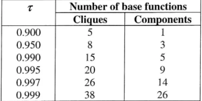
Let us first illustrate how the number of resulting base functions depends on the parameter 1'. This is shown in Table 1, where the number of resulting groups is given for selected values of the 2' for the two partitioning methods described. The effect of changing TiS strongly dependent on the original function set. If, for example, the original functions are less linearly dependent, then a significant reduction in the number of functions may require a much smaller value of 2' compared with the example shown here.

Table 1 Starting from the 61 functions, the table shows how the number of base functions increases with increasing value of the parameter I.

2' Number of base functions

Cliques Components 0.900 5 1 0.950 8 3 0.990 15 5 0.995 20 9 0.997 26 14 0.999 38 26

As we can see, the Cliques method results in more subsets than the Components method. Thus 1' should be chosen smaller for the first method. This effect is expected and in accordance with the definition of 2' for the two methods. In the Components method, there is always a path between functions in the same subset such that the correlation between neighboring functions on the path exceeds T, while the correlation between pairs of functions in general may be less

than 2: In the Cliques method, however, the correlation between any two functions

in a subset always exceeds the tolerance T.

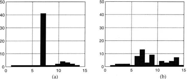
For the following discussion, we considered the fixed value of 2' =0.997 and the 14 base functions resulting from the Components partition method. To each original function there will be an associated base function from which the function itself can be reconstructed. Depending on how functions in the original set are

related to each other, the size of the subsets can vary making the different base

functions associated to a different number of original functions. Figure 2a shows how, in our example, more than half of the original functions are associated with

one of the base functions (number 7), while the other base functions normally are

associated to less than five original functions. In other words, the partition results

in one subset containing more than half of the functions, and otherwise in small

subsets.

For the Cliques method the subsets tend to be more equally sized. Here, with 1

=0.990, the 61 original functions are distributed on 15 subsets, where the largest

contains 13 functions. See figure 2b. In the general case, it is not clear whether equally sized groups are preferable or not. For the Components method, there is obviously a risk for long paths between functions and related base functions in large subsets. In such a case the worst correlation may fall below the tolerance 1'. This is, by definition, not a potential problem in the Cliques method.

0

0*

III;

Figure 2 The number of original functions related to each of base functions for

(a) the Component method (14 base functions for 17:0.997) and (b) the Clique

method (15 base functionsfor 1:0. 990).

15

120

₁₂₀

(a)

_(b)

Figure 3 (a) The reconstruction of an original function from its base function gives negligible error. (b) Reconstruction of the same function by a base function for another subset. As expected, the error is much larger.

In Section 4, we presented two methods for partitioning the set of original

functions into subsets, such that the member functions within a subset are highly

correlated. Given our graph based approach and the tolerance parameter 2', the methods are deterministic and result in proper solutions. Completely different approaches to partition the function may exist, resulting in other partitions.

Any function in a subset can normally be used as a base function for the other members. However, as pointed out in Section 5, the particular choice may have a

clear in uence on the reconstruction error. By the type of active strategies proposed in Section 5, we try to find the most appropriate function to represent the other functions in a subset. Let us now compare some of the heuristics in terms of reconstruction error and minimal correlation coefficient. In order to find

the maximal error, for all functions f,, i:1_,...,N, we compute the best linear

transformation (in least square sense) of the base function fBi associated with fl,

f,- = a

-f...

and take the maximal deviation

maxll f, f, Moo.

1

We also compute the minimal correlation coefficient between each original function and the associated base function. The results are presented separately for the two proposed partition methods in Table 2. As already mentioned, this value typically falls below the tolerance t' for the Components method. Depending on the size of the subsets and the maximum distance from a function to the base function, the minimum correlation coefficient is approximately reduced according to the theorem presented in the end of Section 5. It follows that the minimal correlation coefficient in a subset of n functions is not less than 2' .

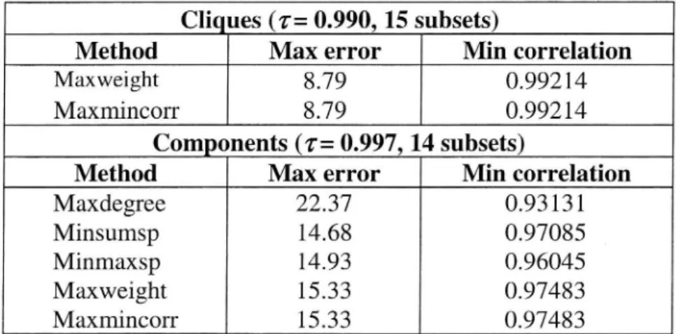
Examining Table l, we see that approximately the same number of base functions can be achieved by choosing 2' = 0.990 for Cliques method, and T = 0.997 for Components method. These values are used for the test results presented in Table 2.

Table 2 Comparison of heuristicsfor choosing basefunctions. The table shows the maximum reconstruction error for any function from its associated base function. We also show the minimum correlation coejficient between functions in

the same subset.

Cliques (1': 0.990, 15 subsets)

Method Max error Min correlation

Maxweight 8.79 0.99214

Maxmincorr 8.79 0.99214

Components (2': 0.997, 14 subsets)

Method Max error Min correlation

Maxdegree 22.37 0.93131

Minsumsp 14.68 0.97085

Minmaxsp 14.93 0.96045

Maxweight 15 .33 0.97483

Maxmincorr 15.33 0.97483

The results in Table 2 suggest that Cliques partitioning is the most suitable method of partitioning for our test case. Now for this method, we present results

concerning how the number of base functions, maximum error, and minimum

correlation vary for different 2' values. For choosing base functions, we use the

maxmincorr method.

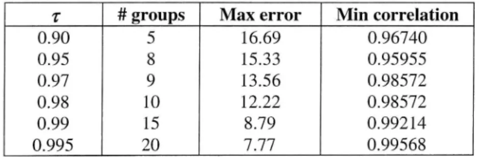
Table 3 E ect of di erent T values in the Cliques partition method proposed in Section 5.

z- # groups Max error Min correlation

0.90 5 16.69 0.96740 0.95 8 15.33 0.95955 0.97 9 13.56 0.98572 0.98 10 12.22 0.98572 0.99 15 8.79 0.99214 0.995 20 7.77 0.99568

Recall that our goal in this example is to reduce the number of functions from 61 to around 20. With 2' = 0.995, this is achieved with very good results by the Cliques method. The base functions chosen from the resulting subsets are actually used in a practical application in Emme/2.

7

Concluding remarks

Based on a practical traffic assignment problem, we have formulated a graph partitioning problem along with the definition of the graph to be partitioned. We have proposed two methods for partitioning and have given test results on how the two methods work on a test case.

Although the Cliques method gives the best results in our tests, we believe both methods to be relevant for different applications. As already mentioned, the problem of finding maximal cliques in a general graph is computationally intractable, whereas finding the connected components is easy. In the problem presented, one might also discuss finding maximum weight cliques, which adds to the complexity of the problem. Components method could be enhanced by dividing large components with long paths into smaller subsets with shorter paths. We believe that the presented graph problem can be subject to interesting further research, and the suggested methods can be improved. To conclude the discussion on graphs, we would like the reader to note the following. The description of the graph model is based on a user defined tolerance bound 1'. Only correlation coefficients of value at least 2' are interpreted as edges of the graph. Another possible way to view this is as a complete weighted graph, where correlation coefficients are the weights on the edges. These two representations are equivalent with respect to the minimization problem stated in Section 4.

For the practical application described in the first section, we have shown that the number of functions that need to be stored in Emma/2 can be reduced to less than a third without introducing unacceptable errors. This has important impacts on the possibilities for using complex and exible functions and still staying within the software limit of 2000 operators. In real applications the traffic net works usually contain many different road types with different ow/speed rela-tions. Moreover, the travelling time depends on the speed on links as well as delays in junctions. This is particularly true for urban networks, where the total junction delay may be a significant part of the total travelling time. By the methods proposed in this paper, we are able to implement complex delay functions for our full set of road types, without violating the operator limit in Emme/2. Another important observation is that functions that are grouped together actually correspond to similar road types. This clearly indicates that the proposed methods are powerful for the given application.

8

References

Bjorck, A (1996). Numerical Methods for Least Squares Problems, SIAM.

Dennis, J. E., Jr (1977). Nonlinear Least Squares , in The State of the Art in Numerical Analysis (D. Jacobs, ed), pp. 269-312, Academic Press, London and New York.

Gower, J .C. (1966). A comparison of Some Methods of Cluster Analysis, Bio

metrics, 23:623-637

INR0 (1991). Emme/2 User s Manual, Montreal, Canada.

Jardine, N. and Sibson R. (1971). Mathematical Taxonomy, John Wiley & Sons Ltd, New York.

Matstoms et a1. (1996). Berakning av volume/delay-funktioner for

natverks-analys, VTI Meddelande 777, VTI, Sweden.

Sheffi,Y (1985). Urban Transportation Networks, Prentice Hall Inc. New Jersey.

The MathWorks Inc. (1992). MATLAB High-Performance Numeric Computa-tion and VisualizaComputa-tion Software, Reference Guide.