Life stage‑specific inbreeding
depression in long‑lived Pinaceae
species depends on population
connectivity
Jon Ahlinder
1*, Barbara E. Giles
2& M. Rosario García‑Gil
3Inbreeding depression (ID) is a fundamental selective pressure that shapes mating systems and population genetic structures in plants. Although it has been shown that ID varies over the life stages of shorter‑lived plants, less is known about how the fitness effects of inbreeding vary across life stages in long‑lived species. We conducted a literature survey in the Pinaceae, a tree family known to harbour some of the highest mutational loads ever reported. Using a meta‑regression model, we investigated distributions of inbreeding depression over life stages, adjusting for effects of inbreeding levels and the genetic differentiation of populations within species. The final dataset contained 147 estimates of ID across life stages from 41 studies. 44 Fst estimates were collected from 40 peer‑reviewed studies for the 18 species to aid genetic differentiation modelling. Partitioning species into fragmented and well‑ connected groups using Fst resulted in the best way (i.e. trade‑off between high goodness‑of‑fit of the model to the data and reduced model complexity) to incorporate genetic connectivity in the meta‑ regression analysis. Inclusion of a life stage term and its interaction with the inbreeding coefficient (F) dramatically increased model precision. We observed that the correlation between ID and F was significant at the earliest life stage. Although partitioning of species populations into fragmented and well‑connected groups explained little of the between‑study heterogeneity, the inclusion of an interaction between life stage and population differentiation revealed that populations with fragmented distributions suffered lower inbreeding depression at early embryonic stages than species with well‑connected populations. There was no evidence for increased ID in late life stages in well‑ connected populations, although ID tended to increase across life stages in the fragmented group. These findings suggest that life stage data should be included in inbreeding depression studies and that inbreeding needs to be managed over life stages in commercial populations of long‑lived plants.
Ever since Darwin investigated the effects of self-fertilising and outcrossing mating systems on offspring vigour1, evolutionary geneticists have recognized that inbreeding depression (ID), or the reduced viability and/or fecun-dity of the offspring of related parents, is a primary selective force driving mating system evolution. ID maintains outbreeding and prevents sexual systems from evolving towards exclusive self-fertilization2,3. Inbreeding is also a concern for breeders and conservationists because of its negative effects on population performance and survival4,5. Whereas the vast majority of studies have focused on shorter-lived plants, considerably less effort has been devoted to studying the effects of ID in long-lived outcrossing species such as trees, and of the work that has been done, almost all have focused on ID in early embryonic stages4,6,7. Even fewer studies have addressed the question of how population size and genetic differentiation affect the strengths of ID across life stages of long-lived species. This lack of knowledge is surprising given the long-standing recognition that tree species should be more favourable than short-lived species as models for studying the cumulative life stage effects of inbreeding on ID4,8.
Theoretical models have identified mating system (i.e., outcrossing versus selfing) as a key determinant of the timing of population ID2,9. Selfers are more often observed to express ID in later life stages (i.e., survival and growth/reproduction) whereas outcrossers exhibit higher ID at either early or both early and late life stages2,5.
OPEN
1Division of CBRN Defence and Security, Swedish Defence Research Agency, 901 82 Umeå, Sweden. 2Department
of Ecology and Environmental Science, Umeå University, 901 87 Umeå, Sweden. 3Department of Forest Genetics
and Plant Physiology, Swedish University of Agricultural Sciences, 901 87 Umeå, Sweden. *email: jon.ahlinder@
Husband and Schemske5 concluded that the early stage ID seen in outcrossing species likely arises from the expression of recessive lethal or strongly deleterious alleles in homozygous form. Early life stage ID should thus be rarer in selfers because homozygotes for deleterious alleles coding for traits expressed at this stage would have been exposed to selection and immediately purged from populations. In contrast, deleterious alleles for genes expressed in later life stages could be maintained in populations as long as they do not affect plant establishment and/or reproduction. Late ID has also been interpreted to be the result of the cumulative effects of smaller fit-ness reductions10 caused by mildly deleterious recessive alleles that are more difficult to purge5. The result, given either of these alternative explanations, should be an increase in late life stage ID in both selfing and outcrossing mating systems.
The strength and timing of ID can also be affected through alterations of the mating system induced by past demographic changes. Geographically restricted and isolated populations descended from species with once large, well-connected outcrossing populations would experience decreases in effective population sizes and
hence increased consanguineous mating11. Relatively soon after population size reduction, progeny would be
expected to suffer from severe ID resulting from increased homozygosity for the deleterious recessive alleles
that had accumulated in the previously large outbreeding populations5. Should inbreeding continue in these
small populations, selective elimination of the deleterious alleles (purging) is expected, leading to reduced levels of ID as observed in species with self-fertilising mating systems2. Purging may not, however, act effectively on fitness traits that are controlled by many genes of small effect or when Ne becomes very small3,12. However, in small populations affected by a longer histories of inbreeding, crossing experiments designed to measure ID in these populations may also fail to detect further reductions in population fitness (ID baseline hypothesis)13. This could lead to the erroneous inference that the apparently low levels of ID were caused by purging (purging hypothesis). Although both hypotheses are possible, their effects on the evolution of population mating system will differ. Under the purging hypothesis, the major force counteracting a transmission advantage of selfing is lost and breeding systems will evolve to allow greater levels of inbreeding or selfing, which would not be the case under the ID baseline hypothesis.
Our study focuses on the family Pinaceae, which, although self-compatible, tend to be highly outcrossing, effectively resulting in large randomly mating populations6. In conifers, most published studies of ID have focused on a single early life stage, most commonly, the high abortion rate of seeds during embryo development14,15. Selec-tive embryo abortion in conifers reduces the impact of genetic load caused by nearly lethal recessive mutations that accumulate during the large number of cell divisions that occur before flowering16. Two factors contribute to the maintenance of the high frequency of recessive mutations in conifers, namely, effective outcrossing facilitated by long distance pollen flow, greater survival of outcrossed progenies and large effective population sizes. In a
review of the literature of ID in conifers, Williams and Savolainen17 concluded, in accordance with theoretical
predictions, that inbreeding effects were most pronounced at early development stages (see also Koelewijn et al.18) although other authors have found increased ID at late developmental stages19. Further effort to investigate the distribution of ID across life stages is thus warranted.
Here we investigate the distribution of ID across four life stages in 18 species of the Pinaceae collected from
41 individual studies. Unlike Husband and Schemske’s meta-analysis of the timing of ID in plants5, our study
is performed on species from a single family (Pinaceae) that share many biological characteristics such as a predominantly outcrossing mating system, wind pollination, long-distance gene flow and long life-span, thus offering a more homogeneous group that can be subdivided into classes based on their population sizes and levels of genetic differentiation. Pinaceae is also characterized by a high lifetime fecundity and large pollen and seed production that permits the abortion of large numbers of inbred seeds without compromising population fitness. A dramatic reduction in population effective size could, however, result in a transition towards a self-ing matself-ing system that would permit, after many generations, the purgself-ing of genetic loads so characteristic of
Pinaceae species20–23. We aim to answer the following questions in this study: (1) how is ID distributed among different life stages of long-lived tree species? How does the inbreeding coefficient affect the distribution of ID across these life stages? (2) Do species with small isolated populations differ in the magnitude and/or timing of ID from those occupying large, continuous areas of distribution?
Results
The final dataset.
First, ID data for 18 species from five genera (Pinus, Abies, Picea, Pseudotsuga and Larix) in the Pinaceae were obtained from 41 studies (Figs. 1, 2, Fig. S1, Table S1), by using the Web of Science database as well as older reports held in plant breeding institutions. In total, 147 estimates of ID were included in the analysis, which makes this one of the more extensive compilations for long-lived perennial species reported in the literature. The 10th, 50th and 90th percentiles of the collected ID estimates corresponded to IDs of 0.03, 0.20 and 0.707, respectively. In addition to ID estimates and their standard errors (SE), data that could explain vari-ation in ID such as inbreeding coefficients (F) and the life stages of the inbred populvari-ations, were collected. The study-specific inbreeding coefficient(s) were obtained from the respective crossing designs performed in each study, resulting in F = {0.125, 0.25, 0.5, 0.75}. For some study-specific configurations (i.e. combinations of life stage, inbreeding coefficient and species fragmentation status), a large number of ID estimates were available: for an inbreeding coefficient of F = 0.5, 99 ID estimates were collected, mostly from self-crossing designs (Fig. S1a); and for the adult vegetative life stage, 69 ID estimates were available (Fig. S1b), in which some ID estimates partly overlapped with the F = 0.5 group. The number of ID estimates within each level of inbreeding coefficient and species distributions were, in some cases, highly unbalanced (Fig. S1a); for example, only two estimates were available for continuously distributed species and F = 0.75. To account for this unbalanced design, a random effects regression model was used to analyse the data.Prior to carrying out the meta-analysis, we tested the data for homogeneity to investigate whether the ID esti-mates from the experiments were sufficiently similar to warrant their combination into an overall effect size term (i.e. a single study-level effect) or whether additional study-level data would improve the analysis. Our hypothesis was that the addition of information, such as crossing-designs, life stages and genetic connectivity for each spe-cies, would explain a greater portion of variation in ID estimates than consideration of individual study-effects alone. There was strong evidence for heterogeneity in the data (Q = 9014, p < 0.001), which supports the addition of the aforementioned species-specific details into the regression analysis. The next step was to decide a suitable way of incorporating the species-specific population sizes and genetic connectivity into the regression analysis.
Barnes (1964) Barnes et al (1962) Bingham (1973)
Bingham & Squillace (1955)
Dieckert (1964) Durel and Kremer (1995) Durel et al (1996)
Geburek (1986)
Griffin and Lindgren (1985) Kormutak and Lindgren (1996) Langner (1959) Pawsley (1964) Sorensen (1999) Wu et al (1998) 0.21 (0.06 to 0.37) 0.23 (0.09 to 0.37) 0.31 (0.28 to 0.34) 0.25 (0.06 to 0.44) 0.31 (0.03 to 0.59) 0.38 (0.29 to 0.47) 0.77 (0.68 to 0.87) 0.47 (0.36 to 0.58) 0.12 (−0.10 to 0.34) 0.11 (0.05 to 0.18) 0.21 (0.08 to 0.34) 0.21 (0.14 to 0.28) 0.11 (−0.02 to 0.24) 0.26 (0.24 to 0.29) 0.38 (0.33 to 0.42) 0.03 (0.00 to 0.06) 0.05 (0.00 to 0.09) 0.00 (−0.04 to 0.04) 0.05 (0.03 to 0.08) 0.10 (0.06 to 0.14) −0.02 (−0.03 to 0.01) 0.07 (0.03 to 0.12) 0.15 (0.12 to 0.18) 0.25 (0.21 to 0.29) 0.20 (0.13 to 0.26) 0.26 (0.23 to 0.30) 0.37 (0.32 to 0.42) 0.35 (0.31 to 0.39) 0.30 (0.27 to 0.33) −0.02 (−0.07 to 0.03) 0.03 (0.00 to 0.06) 0.57 (0.47 to 0.67) 0.58 (0.48 to 0.68) 0.42 (0.28 to 0.56) −0.08 (−0.29 to 0.13) −0.05 (−0.20 to 0.10) 0.14 (0.06 to 0.22) 0.14 (−0.13 to 0.41) 0.33 (0.30 to 0.37) 0.49 (0.45 to 0.53) 0.04 (−0.04 to 0.12) 0.40 (0.29 to 0.50) 0.47 (0.32 to 0.63) 0.04 (−0.04 to 0.12) 0.05 (−0.10 to 0.20) −0.03 (−0.49 to 0.43) 0.06 (−0.15 to 0.27) 0.01 (−0.48 to 0.50) 0.15 (−0.02 to 0.32) 0.07 (−0.38 to 0.52) 0.19 (−0.04 to 0.42) 0.11 (−0.44 to 0.66)
Trial
ID estimate
(SE)
−0.4 0.0 1.0Fragmented distribution
Inb
level
L-h
stage
Species
Categorical coveriate levels:
Inbreeding coefficient: 0.125 0.25 0.50 0.75 Life-history stage: E JV AV AR Pinus monticola Pinus monticola Pinus monticola Pinus monticola Larix deciduas Pinus pinaster Pinus pinaster Picea omorica Pinus radiata Abies alba Picea omorica Pinus radiata Pinus ponderosa Abies procera Pinus radiata
Figure 1. Forest plot of the final dataset including study-specific covariate levels for species with fragmented
population distributions. The x-axis shows the level of ID. Life stage and Inbreeding are abbreviated as L-h and Inb.
0.87 (0.82 to 0.91) 0.82 (0.74 to 0.90) 0.83 (0.76 to 0.90) 0.26 (0.14 to 0.37) 0.60 (0.46 to 0.74) 0.28 (0.18 to 0.39) 0.10 (0.01 to 0.19) 0.18 (−0.37 to 0.55) 0.71 (0.56 to 0.85) 0.53 (0.42 to 0.63) 0.19 (0.04 to 0.35) 0.86 (0.82 to 0.91) 0.08 (−0.16 to 0.24) 0.02 (−0.04 to 0.06) 0.31 (0.24 to 0.38) −0.02 (−0.07 to 0.04) 0.05 (−0.04 to 0.14) 0.27 (0.22 to 0.32) 0.24 (0.09 to 0.39) 0.29 (0.21 to 0.37) 0.44 (0.39 to 0.50) 0.64 (0.57 to 0.71) 0.08 (0.03 to 0.12) 0.72 (0.69 to 0.74) 0.14 (0.13 to 0.14) 0.07 (0.07 to 0.08) 0.13 (−0.07 to 0.33) 0.02 (0.01 to 0.02) 0.17 (0.14 to 0.20) 0.61 (0.53 to 0.69) 0.38 (0.32 to 0.43) 0.39 (0.34 to 0.44) 0.75 (0.69 to 0.81) 0.76 (0.71 to 0.82) 0.01 (−0.34 to 0.36) 0.32 (0.21 to 0.43) 0.20 (−0.05 to 0.45) 0.78 (0.64 to 0.92) 0.16 (0.08 to 0.25) 0.12 (0.04 to 0.19) 0.03 (−0.03 to 0.09) 0.05 (0.00 to 0.10) 0.11 (0.0 to 0.22) 0.33 (0.18 to 0.47) 0.20 (0.15 to 0.25) 0.30 (0.20 to 0.40) 0.25 (0.15 to 0.35) 0.20 (0.13 to 0.28) 0.12 (0.06 to 0.19) 0.12 (0.06 to 0.18) 0.06 (−0.02 to 0.14) 0.30 (0.26 to 0.34) 0.24 (0.17 to 0.30) 0.89 (0.84 to 0.94) 0.54 (0.42 to 0.66) 0.13 (0.04 to 0.22) 0.04 (−0.04 to 0.12) 0.20 (0.17 to 0.23) 0.19 (0.14 to 0.24) 0.55 (0.43 to 0.66) 0.07 (0.02 to 0.13) 0.24 (0.19 to 0.29) 0.82 (0.77 to 0.88) 0.72 (0.66 to 0.78) 0.33 (0.31 to 0.35) 0.29 (0.27 to 0.31) 0.61 (0.43 to 0.78) 0.25 (0.22 to 0.28) 0.44 (0.41 to 0.47) 0.17 (0.11 to 0.23) 0.24 (0.24 to 0.25) 0.18 (0.17 to 0.18) 0.22 (0.21 to 0.22) −0.05 (−0.05 to −0.06) 0.05 (0.02 to 0.09) 0.07 (0.03 to 0.10) 0.15 (0.13 to 0.18) 0.20 (0.17 to 0.23) 0.04 (0.03 to 0.05) 0.14 (0.12 to 0.15) 0.12 (0.02 to 0.21) 0.22 (0.14 to 0.31) 0.44 (0.36 to 0.52) 0.05 (0.02 to 0.08) 0.05 (0.00 to 0.10) 0.05 (−0.01 to 0.11) 0.06 (0.03 to 0.10) 0.06 (0.00 to 0.11) 0.05 (−0.02 to 0.12) 0.18 (0.11 to 0.26) 0.20 (0.10 to 0.29) 0.30 (0.17 to 0.44) 0.31 (0.24 to 0.39) 0.49 (0.40 to 0.57) 0.96 (0.94 to 0.97) Trial ID estimate (SE) −0.4 0.0 1.0 Species L-h stage Inb level
Categorical covariate levels:
Inbreeding coefficient: 0.125 0.25 0.50 0.75 Life-history stage E JV AV AR
Bishir & Namkoong (1987) Coles & Fowler (1976) Cram (1984) Dengler (1939) Dieckert (1964) Ehrenberg et al. (1955) Fowler & Park (1983)
Franklin (1969)
Johnsen et al. (2003) Jonsson (1976) Kormutak et al. (2005) Kraus & Squillace (1964) Layton & Goddard (1983)
Lindgren (1974) Lindgren (1975) Lundkvist et al. (1987) Matheson et al. (1995)
Orr-Ewing (1965)
Park & Fowler (1984)
Plym-Forshell (1974) Skröppa & Tho (1990) Skröppa (1996) Snyder & Squillace (1966) Sorensen (1999)
Sorensen (2001)
Sorensen (1997)
Wang et al. (2004) Woods et al. (2002)
Woods & Heaman (1989) Continuous distribution Pinus taeda Picea glauca Picea pungens Pinus sylvestris Picea abies Pinus sylvestris Picea glauca Pinus taeda Picea mariana Pinus sylvestris Pinus sylvestris Pinus eliotti Pinus eliotti Picea abies Picea abies Pinus sylvestris Pinus eliotti Pseudotsuga menziesii Picea mariana Pinus sylvestris Picea abies Picea abies Pinus eliotti Pseudotsuga menziesii Pinus contorta Pseudotsuga menziesii Pseudotsuga menziesii Pseudotsuga menziesii Pseudotsuga menziesii
Figure 2. Forest plot of the final dataset including study specific covariate levels for species with well-connected
Genetic connectivity data is best utilized by dividing the species into two groups according to
Fst distribution.
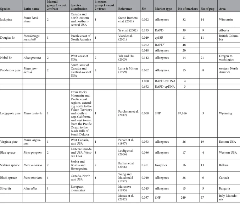
To acknowledge the impact of genetic connectivity on ID, three alternative methods were evaluated. To facilitate this analysis, 44 Fst estimates were collected from 40 peer-reviewed studies for all 18spe-cies included in the study (Table 1, Supplementary information). We hypothesised that the genetic connectivity
of a species could be manifested through the Fst estimates. In addition, the genetic marker type (SNPs, SSRs and Allozymes/Isozymes) used to estimate Fst were noted for each species. To make Fst estimates easier to compare in a single analysis, we included codominant markers based on nuclear DNA and rejected Fst estimates derived from markers that were either dominant (such as RAPD and AFLP) or based on organellar DNA (chloroplast or mitochondria). In model 1, species were partitioned into two groups according to the area of species distribution and level of patchiness. In model 2, a beta regression model and a k-means clustering algorithm were used to partition the species based on their averaged estimates of Fst. This regression-based approach allowed for infer-ring the species effects on Fst while adjusting for the different marker types used to estimate Fst in the respective studies. By adjusting for marker type, we believe that the inferred species effects on Fst would be comparable. In model 3, the posterior mean of the species effect on Fst, obtained from the beta regression model, was used as a covariate.
In model 1, ten species were placed in the partition corresponding to a more continuous (well-connected) area of distribution, while eight were placed in the patchy partition: mean Fst was 0.192 (standard deviation 0.028) and 0.035 (0.001) for the fragmented and continuous distributions, respectively (Table S1). Although this parti-tioning was not strictly based on Fst estimates, the resulting partition corresponded well to average Fst estimates. A beta-regression analysis was then carried out to model the effect of marker types and species on observed Fst values using a Bayesian approach. The result of this regression analysis showed less variation in Fst esti-mates for Isozymes/Allozymes and SSR markers than for SNP-based Fst estiesti-mates, which had greater dispersion (Fig. 3a). As the marker type effects were possible to estimate and had a closed form, we were able to compensate for variation in reported Fst values due to marker system. In other words, by correcting for marker type, we could increase the statistical power in the analysis and more precisely estimate species effects on Fst. The k-means clus-tering of effect size scores of the species predictors in the beta-regression analysis (Fig. 3b) resulted in a partition where, compared to the partitioning in model 1, two species were moved from the fragmented to the continuous group. Larix decidua (average Fst of 0.0625) and Abies alba (average Fst of 0.026), resulting in partition averages
of Fst of 0.241 (0.028) and 0.037 (0.001) for the fragmented and continuous groups, respectively (Fig. 3b). Most
uncertainty in the partitioning occurred for Virginia pine (into the patchy group) and Norway spruce (into the continuous group). The average Fst value increased slightly in both partitions when Fst data were utilized for clustering the species, while the within-group variation decreased slightly (results not shown).
Model performances on the ID data were then compared to decide which result best incorporated species connectivity into the analysis. Based on the predictive performance using two model criteria, LOOIC and LOO,
model 2 outperformed the other models, although model 1 performed almost equally well (Table 2), which is not
surprising given the similarities in species partitioning. This indicates that model 2 represented the best way to incorporate population size and connectivity descriptions of species in the Pinaceae family. Model 3, which used average species effects on Fst as a covariate, performed least well. Thus, the meta-regression model was finalized for further analysis of the ID data by using the partitions of species obtained from model 2.
To make all ID estimates comparable, we included species and study-specific predictors in all models so that any individual species or study effects on ID were accounted for in the regression analysis. Neither the species nor the study predictors showed clear effects on ID (Figs. S3 and S4, respectively) and all credible intervals (CI) contained zero at any relevant confidence level.
ID is most pronounced at highest levels of inbreeding and at early life stages.
Based on the meta-regression analyses using model 2, we first focused on the distribution of ID across inbreeding levels and life stages (and their interactions) of the populations under study. The inbreeding coefficient (denoted F), obtained from the crossing design for each ID estimate, had a strong positive effect on ID (α, Fig. 4, Table S2). In other words, the more inbred a study population, the higher the expected average ID. The 95% CI of the regres-sion coefficient, α, did not contain zero, suggesting that it was beneficial to incorporate crossing design in the analysis through F.The life stage predictor was observed to have a profound effect on ID (β, Fig. 4, Table S2). ID effects were
most positive in the embryonic stage and most negative in the juvenile vegetative growth stage; neither of these uncertainty intervals contained zero (Table S2). Interestingly, of all life stages, only the embryonic stage coeffi-cient was clearly positive, which implies a very strong effect of this life stage on ID. This finding is not surprising as the ID estimates for the earliest stages reported in our raw data were very high, often greater than 0.8 (see e.g. Fig. S1). The adult vegetative and the adult reproductive stages had weak average effects on ID compared to the embryonic and juvenile growth stages, and the 95% CI included zero. However, ID increases with life stage between the juvenile vegetative and final reproductive stages. This trend of increasing levels of ID at later life stages is seen in studies on e.g. Picea glauca24 and Pinus taeda25 (Fig. 2).
Furthermore, an interaction term between F and life stage strongly affected ID (ε, Fig. 4, Table S2). F had a
greater impact on ID at the early embryonic life stage at the 95% significance level, but a reduced impact at the juvenile vegetative growth stage at the 90% significance level. Thus, an increment in F of 0.25 would have very different impact depending on the life stage at which the ID was measured. ID would increase by approximately 0.39 if the study was conducted at the embryonic stage instead of at the juvenile vegetative stage if all other
fac-tors were held constant (i.e. the same species and from the same region). For example, Orr-Ewing26 reported an
increase of 0.35 in ID for Pseudotsuga menziesii from inbreeding levels F = 0.5 and 0.75 at the embryonic stage. Thus, the effect of inbreeding level was unevenly distributed across the two first life stages in the Pinaceae family.
Species Latin name
Manual group 1 = cont
2 = fract Species distribution
k-means group 1 = cont
2 = fract Reference Fst Marker type No of markers No of pop Area
Norway spruce Picea abies 1 Eurasia 1 Unger et al. (2012) 0.002 EST-SSRa 6 3 Austria
Achere et al. (2005) 0.009 SSR 25 3 Europe Achere et al. (2005) 0.029 AFLPb 265 3 Europe Chen et al. (2012) 0.05 SNPc 445 18 Europe Western white
pine Pinus monticola 2
West of North America, One isolated popula-tion in the south
2 Kim et al. (2011) 0.201 AFLP 66 15 Western NA Liu et al. (2011) 0.163 SNP 53 7 Western NA White spruce Picea glauca 1 West/North of North America 1 Namroud et al. (2008) 0.006 SNP 534 6 Québec
Maritime pine Pinus pinaster 2
Western Medi-terranean basin, south Europe and Africa and Atlantic cost of Spain, Portugal and France
2 Wahid et al. (2010) 0.120 ncSSRd 7 10 Marocco
Soto et al. (2010) 0.221 cpSSRe 6 38 Iberia Eveno et al. (2008) 0.150 ncSSR 8 10 Mediterranean coast 0.137 SNP 302 10 Jaramillo-Correa et al. (2015) 0,251 SNP 18 g 36 Mediterranean
European Larch Larix decidua 2 Central Europe, in the moun-tains 1
Wagner et al.
(2012) 0.082 SSR 13 18 Central Europe Mosca et al.
(2012) 0.043 SNP 267 24 Northern Italy Scots pine Pinus sylvestris 1 Eurasia 1 Soto et al. (2010) 0.070 cpSSR 6 30 Iberia
Scalfi et al.
(2009) 0.080 ncSSR 3 3 Italy Kahru et al.
(1996) 0.020 Dvornyk et al.
(2002) 0.017 h SNP 12 3 Finland and Russia 0.11 SNP 12 4 Finland, Russia and Spain Pyhäjärvi et al.
(2007) 0.065 SNP 153 4 Europe Loblolly pine Pinus taeda 1
South east USA Most of it planted after the Great depres-sion
1 Eckert et al. (2010) 0.043 SNP 1730 54 South east UsA
Slash pine Pinus elliottii 1
South east USA. The smallest distribution of the four south USA pines
1 Berg and Ham-rick (1997) 0.028 Allozymes 2 16 South east USA Radiata pine Pinus radiata 2 Cost of Cali-fornia 2 Kahru et al. (2006) 0.140 SSR 19 5 California
Moran et al.
(1988) 0.162 Allozymes 31 5 California Black pine Pinus nigra 2 North Africa, South Europe
and Asia Minor 2
Soto et al.
(2010) 0.136 cpSSR 6 14 Iberia P. pinceana Pinus pinceana 2
Small popula-tion size and endemic species of Mexico
2 Leidig et al. (2001) 0.152 Allozymes 27 8 Mexico Continued
Species with continuous areas of distribution are particularly prone to ID at the embryonic life
stage.
We were particularly interested in whether interactions occurred between life stage and species con-nectivity, which might indicate that evolutionary forces have acted to alter the mating-system in the Pinaceaepopulations. The effect of the species connectivity (γ, Fig. 4, Table S2) shows that a higher ID was observed in
the group with high connectivity, γ1, although at a lower level of confidence (90% CI did not contain zero: Fig. 4,
Table S2). Species-specific population sizes and genetic differentiation thus influenced the strength of ID.
For interactions between life stage and species connectivity (δ, Fig. 4, Table S2), two of eight interaction
group-levels were deemed to be significantly different from zero (i.e. did not include zero at 95% and 90% levels,
respectively). The interaction between the early life stage and well-connected groups (δ11) was higher than the
estimates for all other δ-group levels, indicating that the main predictors alone could not efficiently capture the profound effect of early ID. Clearly, species connectivity accounted for different early life stage ID (δ11 vs δ12) since the effect of the continuous group was particularly high. The reason for this profound effect was the large estimated ID of > 0.8 reported in several studies across a variety of species, e.g. Pinus taeda27 and Picea pungens28 (Fig. 2). In general, if all factors other than species membership in well-connected or fragmented groups were the same in two arbitrary studies, the expected difference in ID would be as large as 0.40, as was often observed (see
Table 1. Species connectivity using the United States Department of Agriculture Natural Resources
Conservation Service (http:// plants. usda. gov/) for the American species and Agro Forestry Tree Database
(http:// www. world agrof orest ry. org/) for European species. References provided in Supplementary information.
a Expressed sequence tags—simple-sequence repeats. b Amplified fragment length polymorphism. c Single
nucleotide polymorphism. d Nuclear simple-sequence repeats. e Chloroplast simple-sequence repeats. f Random
amplification of polymorphic DNA. g Only SNPs associated with climate gradient. h If a single population from
Spain was excluded.
Species Latin name
Manual group 1 = cont
2 = fract Species distribution
k-means group 1 = cont
2 = fract Reference Fst Marker type No of markers No of pop Area
Jack pine Pinus bank-siana 2
Canada and north-eastern and northern-central USA
1 Saenz-Romero et al. (2001) 0.022 Allozymes 82 14 Wisconsin Ye et al. (2002) 0.155 RAPD 39 9 Alberta Douglas fir Pseudotsuga menziesii 1 Pacific coast of North America 1 Viard et al. (2001) 0.019 cpSSR 11 11 British Colum-bia
0.072 RAPDf 48
0.018 Allozymes 20
Nobel fir Abies procera 2 West coast of USA 2 Yeh and Hu (2005) 0.112 Allozymes 14 21 Oregon to washington Ponderosa pine Pinus pon-derosa 2
South-west of Canada and Central-west of USA
2 Latta & Mitton (1999) 0.062 Allozymes 15 8 western North America 1.000 RAPD-mtDNA 4
0.652 RAPD-cpDNA 3
Lodgepole pine Pinus contorta 1
From Rocky Mountain and Pacific coast regions, extend-ing north to the Yukon Territory and south to Baja California, and west to east from the Pacific Ocean to the Black Hills of South Dakota
1 Parchman et al. (2012) 0.008 SNP 97,616 3 Wyoming
Virginia pine Pinus virgini-ana 1 West Canada, east USA 1 Parker et al. (1997) 0.053 Allozymes 26 19 Eastern USA Blue spruce Picea pungens 2 Eastern Canada and USA,
West-ern USA 1
Leidig et al.
(2006) 0.086 Allozymes 17 4 Western USA Serbian spruce Picea omorica 2 Serbia and Bosnia and
Herzegovina 2
Ballian et al.
(2006) 0.261 Isozymes 16 13 Balkan Black spruce Picea mariana 1 Canada, North-east USA 1 Wang and Macdonald
(1992) 0.010 Allozymes 28 6 Canada Silver fir Abies alba 1 European mountains Matusova (1995) 0.015 Allozymes 15 5 Bulgaria
Mosca et al.
differences in ID reported in Figs. 1 and 2). To highlight the influence of population connectivity level on ID at the embryonic life stage, we performed predictions of ID for comparison (Fig. S5). Furthermore, the combination of juvenile vegetative life stage and continuous species connectivity (parameter δ21) resulted in a particularly low
ID, indicating that these populations could have been affected by purging at the embryonic stage. This interaction between juvenile vegetative life stage and high species connectivity on ID (δ21, Fig. 4) is contributed by a
rela-tively large group of studies in, e.g. Pinus sylvestris29 and Pinus taeda25, with reported ID close to zero with n = 10 ID estimates from 9 different studies. Note, however, the outlier ID estimate of 0.71 reported for Picea abies30.
To summarize the meta-regression analyses, the most important finding indicates that Pinaceae populations are particularly vulnerable to ID at the embryonic stage and particularly for species with continuous geographic distributions. Even though all CI contained zero in the fragmented species group (δ12–δ42), it is interesting to
SNP SSR Isozymes/Allozymes −4 0 4 8
a
Picea mariana Abies alba Pinus contorta Picea glauca Pseudotsuga menziesii Pinus elliottii Pinus sylvestris Larix decidua Pinus taeda Picea abies Pinus virginiana Pinus ponderosa Picea pungens Abies procera Pinus monticola Pinus pinaster Pinus radiata Picea omorika 0.00 0.25 0.50 0.75 1.00 Proportion Partition Fragmented Well−connectedb
Figure 3. The results of the beta-regression and clustering of the Pinaceae species into fragmented or
well-connected groups, with: (a) inferred posterior distributions of marker types with 90% CI highlighted in blue, and (b) model 2 approach to partition the species into two groups, where the Serbian spruce was fixed in the patchy partition (because of the highest average Fst) to avoid label switching problems.
Table 2. Model criteria statistics including posterior mean estimates obtained from the RStan analysis.
LOO is abbreviation for leave-one-out cross-validation, LOOIC is the LOO information criterion, ELPD is the expected log pointwise predictive density for a new, simulated, dataset based on the inferred posteriors obtained from the RStan analysis, p is a simulation-estimated effective number of parameters. Standard errors are in parentheses. Higher values of elpd indicate a better predictive performance. The posterior standard
deviations are shown in parentheses and σy is the model residual standard deviation.
Model ELPD LOO p LOO LOOIC σy
1 54.2 54.0 − 108.4 1.28 (0.16) 2 54.9 52.0 − 109.8 1.27 (0.15) 3 52.1 70.2 − 104.2 1.24 (0.17)
note that the means of the distributions of δ (and also ID) increase from the embryonic to the adult reproductive stages. This trend is more like that expected for inbreeding species.
Discussion
Species belonging to the Pinaceae have some of the highest estimates of lethal equivalents and mutational loads ever reported in the literature4, which make these long-lived tree species particularly interesting for longitudinal ID studies. However, because high-quality data from inbreeding experiments are difficult to obtain in long-lived species, meta-analysis of combinations of studies from the literature increases both sample size and power to draw inferences about ID effects at multiple levels. We accounted for several sources of variation that contrib-ute to the level of ID, namely life stage, inbreeding level, species connectivity and importantly, the interactions between species connectivity and life stages and between inbreeding coefficients and life stages. We have revealed the distribution of ID across embryonic, juvenile, adult growth, and reproductive life stages in 18 species of the
Pinaceae (147 estimates from 41 studies), and shown the effects of species-specific population size and
con-nectivity on ID. To arrive at the final regression model, we evaluated three alternative models to account for species size and connectivity by incorporating 44 published estimates of Fst. A particular novelty of our results is the association between the timing of ID and the connectivity of species; inclusion of the interaction terms in the regression model reduced the between-study heterogeneity considerably. We observed a higher level of ID
at the embryonic stage in continuous populations (δ11, Fig. 4) than compared to ID at the embryonic stage in
fragmented populations (δ21, Fig. 4).
It is necessary to recognise several underlying assumptions when interpreting our results. We assumed that the out-crossed, non-inbred reference population used in each study consisted of unrelated trees prior to the inbreeding trials. To reduce biological contributions to bias, we excluded studies having open-pollinated refer-ence populations so that the inbreeding coefficients in the study populations should be as predicted by theory31.
α β1 β2 β3 β4 γ1 γ2 −0.4 −0.2 0.0 0.2 0.4 0.6 a δ11 δ21 δ31 δ41 δ12 δ22 δ32 δ42 ε1 ε2 ε3 ε4 −0.6 −0.3 0.0 0.3 0.6 b
Figure 4. Inferred posterior distributions of regression parameters for all corresponding-group level
predictors included in the meta-regression model. The mean and 90% credible interval (5th and 95th quantiles) are highlighted within the posteriors in blue. In panel a: α corresponds to the effect of inbreeding level of populations on ID, β is the life stage effect (1-embryonic, 2-juvenile vegetative, 3-adult vegetative, 4-adult reproductive), γ is the effect of species connectivity (1-well-connected, 2-fragmented). In panel b: δ is the effect of the interaction life stage × species connectivity, ε is the effect of the interaction inbreeding coefficient × life stage.
However, the population histories of the sampled trees in each individual study may have resulted in some level of relatedness, and consequently, our assumption of a total absence of consanguinity may be incorrect. For example, historically small population sizes cause genes to drift, reducing genetic variation. This reduction in genetic variance increases the likelihood of mating between related individuals and inbreeding in a popula-tion. As a result, the actual difference in inbreeding coefficients between the control and inbred populations might be lower than what is assumed here, which, in turn, might cause an underestimation of the effect of the inbreeding coefficient on ID. This would make it difficult to detect a further reduction in population fitness
fol-lowing experimental selfed crosses. This phenomenon, known as the baseline hypothesis13 induces uncertainty
when interpreting reduced ID in small, fragmented populations as a result of purging. In addition, competition for light, nutrients, water and pollen might intensify the effect of inbreeding on the fitness of individual trees over time, a conclusion drawn in several meta-analytic studies32–34 and in pedigree analyses of natural animal populations35–37. However, Yun and Agrawal38 showed that inbreeding depression was more strongly correlated with density dependence (i.e. competition) than with stressful conditions in Drosophila melanogaster, while
Sandner and Matthies39 showed that most stressful treatments decreased ID (i.e. nutrient limitations) in Silene
vulgaris. See Willi et al.40 for a review of the subject.
In species that have been outcrossing for much of their evolutionary history, the progeny of self-pollinations are expected to suffer severe early ID due to the accumulation of recessive lethals4. This is the case in the family
Pinaceae, where early ID, often measured as proportion of seed abortion, is typically high due to high genetic
load of recessive alleles exposed as homozygotes upon selfing41–43. Husband and Schemske5 reviewed the effects of stage-specific ID in both self- and cross-fertilizing species and found that outcrossing species suffered greater ID at early, seed viability stages than selfing species, a pattern that we also observed in our study. Our results also agree with previous findings in conifers and support much higher ID at the earliest developmental stages17,18,24 (β1, Fig. 4). Our data do not, however, support a clear increase in ID towards reproductive life stages (β2–β4),
indicating that if mutations of mild effect are maintained in later life stages, their effects on ID were not strong enough to be detected.
We utilized Fst information from the literature to partition our species into two groups in which populations were either well-connected over larger areas or occurred as smaller isolated fragments. Species with well-con-nected distributions had lower estimated Fst values (Fst = 0.241 (0.028)) than those with fragmented distributions (Fst = 0.037 (0.001)), providing a plausible way to model the effect of species-specific population distributions on ID. The levels of ID found in well-connected and fragmented species groups (i.e. γ, a main effect in the regres-sion model) showed marginally significant differences. An interesting difference emerged when the interactions
between connectivity and life stage were assessed (δ, Fig. 4). Populations of species with high connectivity
suf-fered more severely from inbreeding effects during the embryonic stage than fragmented populations (δ11 vs.
δ12). The differences in ID between embryonic and juvenile stages in the well-connected species (δ11 vs. δ21) is
likely the result of removal of unfit individuals (i.e. seed abortion), whereas the significantly lower ID observed at the embryonic stage in the fragmented group (δ12 vs. δ12, Fig. 4) may be due to purging that has occurred on
site in previous generations. If purging has occurred, decreased ID during the embryonic stage could drive a transition from an outbreeding mating system, typical of well-connected populations, towards selfing in species with fragmented distributions.
The evolutionary transition from predominantly outcrossing to selfing is known in conifers44. Large, outcross-ing populations maintain substantial ID that acts as a major factor opposoutcross-ing a transition to selfoutcross-ing18,45. When an outcrossing population becomes inbred to a sufficient magnitude over time, selection will favour a selfing
mat-ing system as long as the strength of ID is maintained below a threshold level of 0.546. A number of theoretical
and empirical studies have also stressed that the transition toward selfing in long-lived outcrossed organisms with typically high levels of gene flow is only likely to be initiated where demographic events, such as small population sizes associated with isolation or bottlenecks, act as catalysts18,45,47,48. This is because the transition to selfing requires that selfing individuals survive and reproduce over many generations, which is unlikely to occur in well-connected populations.
Using a theoretical approach, Hedrick et al.49 investigated the effects of multiple genetic factors on the number
of lethal equivalents observed in the northern and southern Scots pine populations in Finland50. The authors
concluded that the reduction in the magnitude of ID in the northern populations may be the result of increased levels of self-fertilization. Furthermore, Vogl et al.20 found evidence for the evolution of the mating system in native populations of Pinus radiata, known to have a history of population bottlenecks, which restricted the species to five small populations. They concluded that purging of early ID was the primary reason for the high proportion of selfed adult trees. Similar findings have been reported in small fragmented populations of Pinus
strobus21, Pinus resinosa22, Picea omorika23 , Pinus contorta51, and Pinus albicaulis52. To summarize the findings in the literature, large differences in mating system and distribution of ID have been detected both within and between populations as functions of population characteristics such as effective size, isolation by distance and demographic history. Hence, it seems likely that the association between the distribution of species and ID found in our analyses could follow from the aforementioned characteristics, but on a wider geographic scale.
We conclude that even if the lower fitness of inbred populations relative to their outcrossing counterparts might be explained by their presumed smaller effective population sizes (high ID baseline), we cannot reject the potential action of purging, which could drive the evolution of the mating system away from predominant outcrossing in the Pinaceae. That the mating system could transition towards increased selfing may be an
evolu-tionary advantage in low density conifer forests or in marginal populations (see Restoux et al.53). Reproductive
assurance accompanying the ability to self might allow colonization of a wider range of environments, a greater tolerance to fluctuations in population size and also allow persistence of Pinaceae species populations. Future studies of this topic would benefit from incorporating detailed data on the distributions and demographic
histories of the species. Estimates of mating system parameters, such as outcrossing rates of the populations, might also be included in the analyses, as in e.g. Duminil et al.54.
Materials and methods
Sampling.
We searched for literature using the Web of Science database for studies of Pinaceae species pub-lished in peer-reviewed journals. We have also included a number of studies from the forest genetics literature representing older, but valuable, work published in conference proceedings and institutional reports of breeding institutes. All studies included in the final data set were required to fulfil the criteria described in the following sections. In short, a study needed to report: (1) an estimate of ID directly or indirectly, via family mean perfor-mance of inbred and non-inbred trees, (2) a measure of deviation around the mean ID estimate either reported directly as standard deviation, variance or coefficient of variance, or indirectly but computable from data in the study.If ID was reported for multiple populations with the same treatment combination (i.e. same species, life stage and inbreeding level), we chose to include only one estimate (with the lowest standard error) to avoid between-population biases50. Because between-family variation in fitness is typically large in inbred populations18,55, stud-ies with inbred and control populations that consisted of fewer than three familstud-ies were not included. When the fitness of each family for inbred and out-crossed populations were only available in graphs, we used Data Theft 3 (http:// datat hief. org/) to estimate ID. To estimate the standard error in ID when only errors of the phenotypes of different families in the populations were reported, a first order Taylor series approximation was used. Because so few studies have reported within-family variation in fitness, we only acknowledged the between-family vari-ation in our analyses (as standard errors).
Definition of ID.
The distribution of ID across life stages was examined by considering stage specificesti-mates obtained from each population. Following Husband and Schemske5, we define stage specific ID at life
stage yi = 1 − (woi/wsi), i = 1,2,3,4, where woi and wsi are the fitnesses of the outcrossed and inbred populations, respectively.
The inbred populations represent four classes of crossing designs: half-sib, full-sib, one and two generations of selfing, which result in inbreeding coefficients, F = 0.125, 0.25, 0.5, 0.75, respectively. The advantage of only using populations derived from controlled crosses is that more precise measures of inbreeding are obtained than
can be estimated from indirect measures such as outcrossing rate from molecular marker data56. Backcross and
full-sib matings were treated in the same class of crossing design since both have an average inbreeding coef-ficient of F = 0.25. Similarly, populations obtained from one generation of selfing and one generation of selfing and additional full-sib crosses, were treated as a crossing design with F = 0.5. We rejected studies with open-pollinated control populations since these contain an unknown proportion of inbred individuals4,49,57 and hence have different levels of F relative to studies where control populations were created by controlled outbreeding. Furthermore, we assume that base populations in each study consisted of unrelated and non-inbred trees, prior to the creation of the inbred population. Even though some material might be sampled from breeding populations selected according to specific breeding objectives, most tree breeding programs worldwide are in their infancy and hence consist of unrelated trees7.
Definition of life stages.
We followed Greenwood58 to define life stages as (1) embryonic (2) post-embry-onic juvenile vegetative, (3) adult vegetative, and (4) adult reproductive stages. The first life stage contained seed quality traits: percentage of sound seeds, sound seeds per cone and total number of sound seeds. Due to parthenocarpy (production of fruit without fertilization of ovules), those individual studies that reported the percentage of sound seeds in Abies, Larix, Picea and Pseudotsuga, may contribute to an overestimation of the level of early ID.The second life stage comprised germination-related traits expressed in the first year after sowing. These traits were germination as percentage of sown seeds, hypocotyl height and germination rate in days. The post-germination stages were divided into pre-reproductive and post-reproductive stages. Since most studies reported either height of the trunk, diameter at breast height and/or survival after planting in the field trial, we included these vegetative traits as measures of fitness, since use of commonly reported traits facilitated a better comparison between species and populations. Stem volume and sectional area were not considered in our analyses because as functions of power of height and diameter, respectively, ID appears to be much higher than those reported
for height and diameter59. We chose the age of reproduction to be 12 growing seasons so that estimates of ID
were placed in either the pre-flowering (embryonic, post-embryonic juvenile vegetative and adult vegetative) or post-flowering (adult reproductive) stages, depending on the age of the population. We acknowledge that it is not strictly accurate to choose a fixed age of reproduction for all species and populations because reproductive age may vary with environmental factors (i.e. climate, water and nutrition supply and competition effects) and the demographic history of the population.
Modelling the effect of species distribution.
We present three alternative ways to model the available species distribution data. In the first model, denoted model 1, estimates of inbreeding effects obtained from species with typically fragmented population distributions were treated as one group while species with large continuous distributions were treated as a second group, based on the species distribution area data from UnitedStates Department of Agriculture Natural Resources Conservation Service (http:// plants. usda. gov/) for North
American species and Agro Forestry Tree Database (http:// www. world agrof orest ry. org/) for European species.
As an alternative to this partitioning, published estimates of Fst for each species were collected. We interpret high
while the opposite is assumed for low values of Fst (low levels of genetic differentiation and a substantial gene
flow between sub-populations). If a difference between the groups is detected in the meta-regression analysis, we can infer that distribution area, our proxy for population size, explains a portion of the variability in ID esti-mates. In model 2, as an alternative way to partition the species into two groups, we made use of k-means cluster-ing, based on pair-wise Fst between species, implemented in the R software60. This method (denoted as model 2)
to partition the species minimizes the within-group variability while maximizing the between-group variability in Fst and does not require any prior knowledge about the area of distribution. This allows the number of species
in each partition to be unbalanced, unlike in model 1. A beta regression model was used to infer the effects of each species on the Fst estimate (i.e. the response variable), which is a proportion of the between subpopulation
genetic variation and the genetic variation in the total population. This model was implemented following the
parametrization suggested by Ferrari and Cribari-Neto61. Such a model had the advantage of allowing us to
cor-rect for the typical behaviour of a response of proportions and can incorporate the different marker types used to estimate the Fst. Only Fst estimates based on SNPs, nucleus SSR and Isozymes/Allozymes were included. After the
regression analysis, we randomly drew 10,000 species effect size values from the inferred posterior of each spe-cies and performed k-means clustering for 10,000 repetitions (and thereby acknowledge uncertainty inherited from the regression into the clustering). Interested readers are invited to see https:// github. com/ jonha r97/ Pinac eae- meta- regre ssion for further details into the beta regression analysis including source code. Finally, in model 3, the mean of the obtained posterior of the species effect on Fst estimates from the beta regression model were
used directly as a covariate in the regression model.
We made use of predictive model selection criteria to identify the preferred regression model (i.e. how to infer the effect of species distribution on ID): leave-one-out cross-validation (LOO) and the LOO information
criterion (LOOIC). LOO and LOOIC scores for the included models were computed within the R package ‘loo’62.
Meta‑regression model.
Our goal is to acknowledge the sources of variation in ID estimates among the set of empirical studies and to infer the effect of life stages and species-specific population distributions on ID. Prior to carrying out the meta-regression analysis, we tested the data for homogeneity following Costa-Font et al.63. Under the null hypothesis of homogeneity, Q is distributed as χ2N − 1 where N is the sample size (i.e.number of ID estimates). To analyse the meta-regression data set, we modelled inbreeding level as a covariate, since the inbreeding coefficient values are directly comparable between crossing designs. Life stage, species-spe-cific population distribution and an interaction term between life stage and species-spespecies-spe-cific population distribu-tion were given group-level labels and were thus modelled as categorical factors. This set of terms (predictors) represented the independent variables in the regression model and allow us to account for heterogeneity arising from study specific details, such as study design. The levels of inbreeding were: F = (0.125, 0.25, 0.5, 0.75), and the corresponding regression coefficient is denoted by α. Regression coefficients for life stages are denoted by
βl, l = 1,…,4 (in the same order as defined in definition of life stages above). These two predictors were
identi-cal in all models considered. Species distributions are denoted γm, m = 1, 2, for well-connected and fragmented
distributions, respectively; the interaction term life stage x species connectivity level is denoted δlm, l = 1,…,4 and m = 1, 2 (for models 1 and 2), and the interaction term inbreeding level x life stage is denoted εl, l = 1,…,4. In model 3, a vector of Fst values was used where each entry corresponds to each ID estimate and the interaction was a combination of the Fst covariate and the life stage factor. The group level effects, a mixture of within- and across-study relationships with inbreeding estimates, are assumed to follow a normal distribution with constant mean and precision. The study effects are denoted by aj[i], j = 1, …,41, and considered to be normally distributed
with variance σa2 and with mean centred around zero because an overall intercept is already included in the
model, and i is the i:th ID estimate within group j. The species effects are denoted by bo[i], o = 1,…,18, again with mean centred around zero and variance σb2. Thus, both aj[i] and bo[i] are assigned varying intercepts for each group (i.e. study and species, respectively) which allows for correlation in ID within groups. All standard devia-tion parameters are assigned a uniform prior. As suggested by Smith et al.64, the student-t distribution was used as a population distribution for ID in the meta-analysis. Prior for degrees of freedom in Student’s t distribution
was assumed to follow a gamma (2,0.1) distribution as proposed by Juárez and Steel65. The non-nested multilevel
meta-regression model we used in the analysis (i.e. models 1 and 2) can be written as:
where μ is the overall mean, SEijklm is the standard error of the i:th ID estimate, df and ηijklm are the degrees of freedom and weighted standard deviation of the t distribution, respectively. For identifiability of the group-level regression coefficients, a hard constraint was imposed by setting the sum to zero for each set of coefficients belonging to the same predictor: ∑βi = 0, ∑γi = 0, ∑δi = 0, and ∑εi = 0, summarized over all group levels i. For model 3, γm and δlm were instead a covariate and a covariate × factor interaction, respectively, with correspond-ing posterior mean of the Fst predictor for each species as obtained in the beta regression analysis described in the “Modelling the effect of species distribution” section. Two levels of significance of the regression coefficients were defined: significant if the zero was outside the 95% credible interval (CI), and marginally significant if the zero was outside the 90% CI. Predictions of ID were made using the Student-t distribution with the inferred regression coefficients and assuming an average study and species effects as parameters. The regression models
yijklm∼t �ijklm, ηijklm,df ,
�ijklm=µ + α + βl+γm+δlm+εl+aj[i]+bo[i], ηijklm=σySEijklm,
aj∼N 0, σa2 , j = 1, . . . , 41,
bo∼N 0, σb2 , o = 1, . . . , 18,
were implemented and analysed through the RStan software66. Default parameters controlling the collection of
Monte Carlo chain samples were used. Forest plots were generated in R60 using function forest.plot.or available
at: http:// www. medic ine. mcgill. ca/ epide miolo gy/ joseph/ pbeli sle/ forest- plot. html, and modified to add group-level covariates data. Density plots of inferred posterior distributions of all regression coefficients in the model
were created using the R-package bayesplot67. More information about analysis details and data is provided at
https:// github. com/ jonha r97/ Pinac eae- meta- regre ssion, and in Table S1.
Data availability
The data are provided in Table S1 and at https:// github. com/ jonha r97/ Pinac eae- meta- regre ssion.
Received: 8 July 2020; Accepted: 6 April 2021
References
1. Darwin, C. Geological Observations on the Volcanic Islands and parts of South America Visited During the Voyage of H.M.S. ‘Beagle’. (Smith, Elder and Co. London., 1876).
2. Lande, R. & Schemske, D. W. The evolution of self-fertilization and inbreeding depression in plants. I. Genetic models. Evolution
(N. Y). 39, 24–40 (1985).
3. Byers, D. & Waller, D. M. Do plant populations purge their genetic load? Effects of population size and mating history on inbreed-ing depression. Annu. Rev. Ecol. Syst. 30, 479–513 (1999).
4. Charlesworth, D. & Charlesworth, B. Inbreeding depression and its evolutionary consequences. Annu. Rev. Ecol. Syst. 18, 237–268 (1987).
5. Husband, B. C. & Schemske, D. W. Evolution of the magnitude and timing of inbreeding depression in plants. Evolution (N. Y). 50, 54–70 (1996).
6. Franklin, E. C. Survey of mutant forms and inbreeding depression in species of the family Pinaceae. in Southeast For. Exp. Station.
USDA For. Serv. Res. Pap. SE, 61 (1970).
7. White, T., Adams, W. & Neale, D. Forest Genetics (CABI Publishing, 2007).
8. Charlesworth, D. & Willis, J. H. The genetics of inbreeding depression. Nat. Rev. Genet. 10, 783–796 (2009).
9. Barringer, B. C. & Geber, M. A. Mating system and ploidy influence levels of inbreeding depression in Clarkia (Onagraceae).
Evolution 62, 1040–1051 (2008).
10. Wolfe, L. M. Inbreeding depression in hydrophyllum appendiculatum: role of maternal effects, crowding, and parental mating history. Evolution (N. Y). 47, 374–386 (1993).
11. Aldrich, P. R. & Hamrick, J. L. Reproductive dominance of pasture trees in a fragmented tropical forest mosaic. Science 281, 103–105 (1998).
12. Frankham, R., Gilligan, D. M., Morris, D. & Briscoe, D. A. Inbreeding and extinction: effects of purging. Conserv. Genet. 2, 279–284 (2001).
13. Angeloni, F., Ouborg, N. J. & Leimu, R. Meta-analysis on the association of population size and life history with inbreeding depres-sion in plants. Biol. Conserv. 144, 35–43 (2011).
14. Sorensen, F. The roles of polyembryony and embryo viability in the genetic system of conifers. Evolution (N. Y)/ 36, 725 (1982). 15. Ferriol, M., Pichot, C. & Lefèvre, F. Variation of selfing rate and inbreeding depression among individuals and across generations
within an admixed Cedrus population. Heredity (Edinb). 106, 146–157 (2011). 16. Klekowski, E. J. Genetic load and its causes in long-lived plants. Trees 2, 195–203 (1988).
17. Williams, C. & Savolainen, O. Inbreeding depression in conifers: implications for breeding strategy. For. Sci. 42, 102–117 (1996). 18. Koelewijn, H., Koski, V. & Savolainen, O. Magnitude and timing of inbreeding depression in Scots pine (Pinus sylvestris L.).
Evolu-tion (N. Y). 53, 758–768 (1999).
19. Wu, H. X., Matheson, A. C. & Spencer, D. Inbreeding in Pinus radiata. I. The effect of inbreeding on growth, survival and variance.
TAG Theor. Appl. Genet. 97, 1256–1268 (1998).
20. Vogl, C., Karhu, A., Moran, G. & Savolainen, O. High resolution analysis of mating systems: inbreeding in natural populations of
Pinus radiata. J. Evol. Biol. 15, 433–439 (2002).
21. Rajora, O. P., Mosseler, A. & Major, J. E. Mating system and reproductive fitness traits of eastern white pine (Pinus strobus) in large, central versus small, isolated, marginal populations. Can. J. Bot. 80, 1173–1184 (2002).
22. Boys, J., Cherry, M. & Dayanandan, S. Microsatellite analysis reveals genetically distinct populations of red pine (Pinus resinosa,
Pinaceae). Am. J. Bot. 92, 833–841 (2005).
23. Kuittinen, H. & Savolainen, O. Picea omorika is a self-fertile but outcrossing conifer. Heredity (Edinb). 68, 183–187 (1992). 24. Fowler, D. P. & Park, Y. S. Population studies of white spruce. I. Effects of self-pollination. Can. J. For. Res. 13, 1133–1138 (1983). 25. Franklin, E. C. Inbreeding as a means of genetic improvement of loblolly pine. in Proceedings of the Tenth Southern Conference on
Forest Tree Improvement 107–115 (1969).
26. Orr-Ewing, A. Inbreeding and single crossing in Douglas-Fir. For. Sci. 11, 279–290 (1965).
27. Bishir, J. & Namkoong, G. Unsound seeds in conifers—estimation of numbers of lethal alleles and of magnitudes of effects associ-ated with the maternal parent. Silvae Genet. 36, 180–184 (1987).
28. Cram, W. H. Some effect of self-pollination, cross-pollination, and open-pollination in Picea pungens. Can. J. Bot. 62, 392–395 (1984).
29. Kormutak, A., Ostrolucka, M., Vookova, B., Pretova, A. & Feckova, M. Artificial hybridization of Pinus sylvestris L. and Pinus mugo Turra. Acta Biol. Cracoviensia Ser. Bot. 47, 129–134 (2005).
30. Dieckert, H. Some investigations on self sterility and inbreeding in spruce and larch. Silvae Genet. 13, 77–86 (1964). 31. Lynch, M. & Walsh, B. Genetics and Analysis of Quantitative Traits (Sinauer Assocs., Inc., 1998).
32. Crnokrak, P. & Roff, D. A. Inbreeding depression in the wild. Heredity (Edinb). 83(Pt 3), 260–270 (1999).
33. Armbruster, P. & Reed, D. H. Inbreeding depression in benign and stressful environments. Heredity (Edinb). 95, 235–242 (2005). 34. Boakes, E. H., Wang, J. & Amos, W. An investigation of inbreeding depression and purging in captive pedigreed populations.
Heredity (Edinb). 98, 172–182 (2007).
35. Keller, L. F., Reid, J. M. & Arcese, P. Testing evolutionary models of senescence in a natural population: age and inbreeding effects on fitness components in song sparrows. Proc. Biol. Sci. 275, 597–604 (2008).
36. Fox, C. W. & Stillwell, R. C. Environmental effects on sex differences in the genetic load for adult lifespan in a seed-feeding beetle.
Heredity (Edinb). 103, 62–72 (2009).
37. Grueber, C. E., Laws, R. J., Nakagawa, S. & Jamieson, I. G. Inbreeding depression accumulation across life-history stages of the endangered Takahe. Conserv. Biol. 24, 1617–1625 (2010).
38. Yun, L. & Agrawal, A. F. Variation in the strength of inbreeding depression across environments: effects of stress and density dependence. Evolution (N. Y). 68, 3599–3606 (2014).
39. Sandner, T. M. & Matthies, D. The effects of stress intensity and stress type on inbreeding depression in Silene vulgaris. Evolution
(N. Y). 70, 1225–1238 (2016).
40. Willi, Y., Van Buskirk, J. & Hoffmann, A. A. Limits to the adaptive potential of small populations. Annu. Rev. Ecol. Evol. Syst. 37, 433–458 (2006).
41. Sorensen, F. Embryonic genetic load in coastal Douglas-Fir Pseudotsuga menziesii var. Menziesii. Am. Nat. 103, 389–398 (1969). 42. Koski, V. Embryonic lethal of Picea abies and Pinus sylvestris. Commun. Instituti For. Fenn. 75, 1–30 (1971).
43. Franklin, E. Genetic load in loblolly pine. Am. Nat. 106, 262–265 (1972).
44. Baker, H. G. Self-compatibility and establishment after ‘long-distance’ dispersal. Evolution (N. Y). 9, 347 (1955).
45. Winn, A. A. et al. Analysis of inbreeding depression in mixed-mating plants provides evidence for selective interference and stable mixed mating. Evolution (N. Y). 65, 3339–3359 (2011).
46. Schemske, D. W. & Lande, R. The evolution of self-fertilization and inbreeding depression in plants. II. Empirical observations.
Evolution (N. Y). 39, 41–52 (1985).
47. Petit, R. J. & Hampe, A. Some evolutionary consequences of being a tree. Annu. Rev. Ecol. Evol. Syst. 37, 187–214 (2006). 48. Scofield, D. G. & Schultz, S. T. Mitosis, stature and evolution of plant mating systems: low-Φ and high-Φ plants. Proc. R. Soc. B
Biol. Sci. 273, 275–282 (2006).
49. Hedrick, P., Savolainen, O. & Kärkkäinen, K. Factors influencing the extent of inbreeding depression: an example from scots pine.
Heredity (Edinb). 82(Pt 4), 441–450 (1999).
50. Kärkkäinen, K., Koski, V. & Savolainen, O. Geographical variation in the inbreeding depression of Scots pine. Evolution (N. Y). 50, 111–119 (1996).
51. Sorensen, F. Effect of Population Outcrossing Rate on Inbreeding Depression in Pinus contorta var. murrayana Seedlings. Scand.
J. For. Res. 16, 391–403 (2001).
52. Bower, A. D. & Aitken, S. N. Mating system and inbreeding depression in whitebark pine (Pinus albicaulis Engelm). Tree Genet.
Genomes 3, 379–388 (2007).
53. Restoux, G. et al. Life at the margin: the mating system of Mediterranean conifers. Web Ecol. 8, 94–102 (2008).
54. Duminil, J., Hardy, O. J. & Petit, R. J. Plant traits correlated with generation time directly affect inbreeding depression and mating system and indirectly genetic structure. BMC Evol. Biol. 9, 177 (2009).
55. Fox, C. W., Scheibly, K. L. & Reed, D. H. Experimental evolution of the genetic load and its implications for the genetic basis of inbreeding depression. Evolution (N. Y). 62, 2236–2249 (2008).
56. Pemberton, J. M. Wild pedigrees: the way forward. Proc. Biol. Sci. 275, 613–621 (2008).
57. Kärkkäinen, K. & Savolainen, O. The degree of early inbreeding depression determines the selfing rate at the seed stage: model and results from Pinus sylvestris (Scots pine). Heredity (Edinb). 71, 160–166 (1993).
58. Greenwood, M. S. Juvenility and maturation in conifers: current concepts. Tree Physiol. 15, 433–438 (1995).
59. Johnsen, K., Major, J. E. & Maier, C. A. Selfing results in inbreeding depression of growth but not of gas exchange of surviving adult black spruce trees. Tree Physiol. 23, 1005–1008 (2003).
60. R Core Team. R: A language and environment for statistical computing. R Foundation for Statistical Computing, Vienna, Austria.
https:// www.R- proje ct. org/. (2020).
61. Ferrari, S. & Cribari-Neto, F. Beta regression for modelling rates and proportions. J. Appl. Stat. 31, 799–815 (2004).
62. Vehtari, A., Gelman, A. & Gabry, J. Practical Bayesian model evaluation using leave-one-out cross-validation and WAIC. Stat
Comput 27, 1413–1432.https:// doi. org/ 10. 1007/ s11222- 016- 9696-4. (2017).
63. Costa-Font, J., Gemmill, M. & Rubert, G. Biases in the healthcare luxury good hypothesis? A meta-regression analysis. J. R. Stat.
Soc. Ser. A Stat. Soc. 174, 95–107 (2011).
64. Smith, T. C., Spiegelhalter, D. J. & Thomas, A. Bayesian approaches to random-effects meta-analysis: a comparative study. Stat.
Med. 14, 2685–2699 (1995).
65. Juárez, M. A. & Steel, M. F. J. Model-based clustering of non-gaussian panel data based on skew-t distributions. J. Bus. Econ. Stat. 28, 52–66 (2010).
66. Carpenter, B. et al. Stan: a probabilistic programming language. J. Stat. Softw. 76, 1–32 (2017).
67. Gabry, J., Simpson, D., Vehtari, A., Betancourt, M. & Gelman, A. Visualization in Bayesian workflow. arXiv 2, (2017).
Acknowledgements
This work was initiated when JA (formerly Hallander) was a postdoc at the Swedish University of Agricultural Sciences, department of Forest Genetics and Plant Physiology. We are grateful to Dag Lindgren, Mikko J Sil-lanpää, Stacey Thompson and Douglas Scofield for sharing data and giving useful comments on the text, and to Patrick Belisle for help regarding the forest plot function. In addition, we thank the reviewer and the associate editor for giving comments that improved the paper. This work was supported by the Kempe Foundation through the Research School in Forest Genetics and Breeding at The Swedish University of Agricultural Sciences (SLU).
Author contributions
J.A., B.E.G. and R.G.G. designed the study, collected the data and wrote the manuscript. J.A. implemented the statistical model and analysed the data.
Competing interests
The authors declare no competing interests.
Additional information
Supplementary information The online version contains supplementary material available at https:// doi. org/ 10. 1038/ s41598- 021- 88128-4.
Correspondence and requests for materials should be addressed to J.A.
Reprints and permissions information is available at www.nature.com/reprints.
Publisher’s note Springer Nature remains neutral with regard to jurisdictional claims in published maps and