Agent-Based Decision Support in Maintenance Service
Operations
Per Hilletofth1*, Lauri Lättilä2, Sandor Ujvari3, and Olli-Pekka Hilmola4
1*
Corresponding author, Logistics Research Centre, School of Technology and Society, University of Skövde, SE-541 28 Skövde, Sweden, E-mail: per.hilletofth@his.se
2
Lappeenranta University of Technology, Kouvola Unit, Finland, Prikaatintie 9, FIN-45100 Kouvola, Finland, E-mail: lauri.lattila@lut.fi
3
Logistics Research Centre, School of Technology and Society, University of Skövde, SE-541 28 Skövde, Sweden, E-mail: sandor.ujvari@his.se
4
Lappeenranta University of Technology, Kouvola Unit, Finland, Prikaatintie 9, FIN-45100 Kouvola, Finland, E-mail: olli-pekka.hilmola@lut.fi
Abstract
In this research an agent-based decision support system for service related maintenance has been developed, the maintenance planning is complex including corrective and preventive tasks of several non-associated plants. This type of problem is well suited for modeling and implementation using Agent-Based Modeling and Simulation (ABMS). The simulation model enables decision-makers to iteratively set parameters, run simulations and evaluate results. Research shows that this approach can improve the understanding of the problem domain and also generate a basis for decision-making. Keywords: Service operations, Decision support, Agent-based modeling and simulation
Introduction
Outsourcing of maintenance involves the use of external companies, referred to as Maintenance Service Providers (MSP); MSPs can encompass the entire maintenance function or select activities. Provided services can either be corrective, preventive or conditional (Garg and Deshmukh, 2006). MSPs are subject to a rapidly changing business environment strongly influenced by the Forrester Effect of non-stock production (Akkermans and Vos 2003), and research shown that information is vital in avoiding up- and down swings in resource needs. Additionally, operations need to be well balanced in terms of utilization rate of personnel (hours billed divided by hours worked) versus service rate towards customers. Another important topic is to keep a balance between maintenance cost and the up-time of the customers’ production systems. Reality is that MSPs also serve other customers in various geographical locations, and these can have long-term contracts for service levels.
One way to improve decision-making is to generate business intelligence by fusing large amounts of data from various sources (Information Fusion, IF). The purpose of IF is typically to extract relevant information from several sources with known certainty to make better decisions than if fusion was not used. It can be defined as “the study of
effective support for human or automated decision-making” (Boström et al., 2007). One method to realize IF in complex industrial environments, which normally is not highlighted as an IF method, is Agent-Based Modeling and Simulation (ABMS). It is related to IF in the way that information from different sources are collected and fused in a synergistic manner into a situation image that provides effective support for human decision-making. Empirical studies have shown that managers aided by agent-based simulations can benefit in several ways (Nilsson and Darley, 2006).
In this research work an agent-based simulation model of service related maintenance has been developed. The simulation model is inspired by an actual case company, e.g. some stochasticity estimates are gained from the case company, but additional data has also been used. Empirical data was collected during a three year period (2006-2008) from various sources including databases, interviews, observations, and internal documents. In the simulation model, the service order fulfilment process is managed by a set of agents that are responsible for one or more activity. It comprise a complex service network (more than 25 customer factories), which is modeled using one common type of industrial machine (CNC) to be served. Provided maintenance service was categorized as either corrective or planned maintenance; the resource expertise needed was categorized into two classes as well, mechanical and electrical. Whole model was built with Anylogic software. The overall purpose of this simulation model is to increase the understanding of the problem domain and to form a basis for better decision-making (i.e. constitute a decision support system), thus improving performance in MSP environment.
The remainder of this paper is structured as follows: In Section 2, the concept of agent-based decision support is discussed through existing literature. Thereafter, in Section 3 the research environment is presented. In Section 4, the simulation model is discussed while some initial simulation results are presented in Section 5. In final Section 6, research is concluded and further research avenues are proposed.
Agent-Based Decision Support
ABMS represents a new paradigm in modeling and simulation, especially suited for complex and dynamic systems distributed in time and space (Lim and Zhang, 2003). It implies that the real (observed) system of interest is modeled in form of a set of interacting agents within a certain environment (i.e. as an agent system) and implemented in simulation software, resulting in an agent-based simulation model/application (Figure 1). An agent system consists of a couple of individual agents with specified relationships to one another within a certain environment. The agents are presumed to be acting in what they perceive as their own interests, such as economic benefit (i.e. they have individual missions), and their knowledge regarding the entire system (i.e. other agents and environment) is limited (Macal and North, 2006). Still, the most important feature in an agent system is the agents’ ability to collaborate, coordinate and interact with each other as well as with the environment to achieve common goals. By sharing information, knowledge, and tasks among the agents in the system, collective intelligence may emerge that can not be derived from the internal mechanism of an individual agent. Furthermore, the ability to coordinate makes it possible for agents to coordinate their actions among themselves, i.e. taking the effect of another agent’s actions into account when making a decision about what to do. The term Multi-Agent System (MAS) is commonly used for agent systems including several interacting and collaborating agents.
Figure 1 – The process of agent-based modeling and simulation
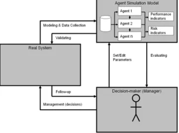
Agent-based simulation can be used to simulate the actions and interactions of individual agents in an agent system to evaluate the agents’ effects on the system as a whole as well as to evaluate the system in general. This implies that an agent-based simulation model can be used as a decision support system (Figure 2). The simulation model consists of the interacting agents and some performance and risk indicators. The utilized data in the simulation model can be collected from databases, observations, interviews or documents in the real system. Decision-makers, can set parameters in the simulation model, run the simulation and evaluate the results. Based on the retrieved information/knowledge they can make decisions regarding how to handle the real system. They could also continually alter different parameters and simulate again to evaluate different management alternative. This implies that an agent-based decision support system fuses information from different sources in a synergistic manner into a situation image that provides effective support for human decision-making. Therefore, it could be regarded as an IF method.
Figure 2 – Agent-based decision support system
Nilsson and Darley (2006) conclude in their empirical study that decision-makers aided by agent-based simulations can benefit in several ways: (1) help them acquire an increased understanding of the impact of unscheduled factors (e.g. breakdowns, accidents, demands change), (2) guide decision-makers’ instinct, since interactive agents generate an emergent pattern, which can be explained and understood and therefore beneficial for the improvement of decision-making in companies and (3) help decision-makers to find where the highest leverage is to be gained among improvement alternatives.
Even if the interest in implementing agent models in various types of business is increasing (e.g. Albino et al., 2007; Chen et al., 2008; Hilletofth, 2007; Shen et al.,
experiments and developed systems have been reported in the academic literature. Davidsson et al. (2005) reviewed the maturity of agent approaches presented in the literature and used the following four main levels: (1) conceptual proposal, (2) simulation experiment, (3) field experiment, and (4) deployed system. In their sample of 56 journal articles published between 1992 and 2005, it was only identified one level 4 and three level 3 research works. A more recent literature review confirms that this situation still exists (Hilletofth et al., 2009); only one manuscript from 33 journal articles published during 2000-2008 included empirically verified results after the implementation of agent-based models. Furthermore, this literature review showed that only small amount of research works were based on real-life observations or systems. Research Environment
In this research work an agent-based simulation model for service related maintenance has been developed. It is inspired by an actual case company but additional data has also been used. The case company tries to manage all customer orders and inquires through a service central. The service central primary works with orders and inquires concerning operative maintenance. These types of orders stand for a big share of the total amount of orders. However, the service central also answer question concerning product and service assortment and guide customer in the organization. Only maintenance coordinators are connected to the service central: which implies that customer asking for other services is further guided in the organization. Customer orders and inquires concerning other services than operative maintenance go through sales department, which handles customer contacts and communicates with different coordinators in the organization. The maintenance coordinators are responsible for the weekly maintenance planning as well as for day-to-day planning. This implies that they determine which technicians that should be assign to which tasks. Currently the organization is divided into two divisions, mechanical and electrical maintenance. The technicians are responsible for conducting the tasks and also reporting what have been done. Currently the reported information mostly concerns information for invoicing.
The case company has identified the service fulfillment process and its management to be one of the most important improvement areas. It has been recognized that there is a need to change the service organization. The company wants to manage all orders and inquires, irrespective of type, through a sales and service central in order to make the operations more efficient (optimize resource utilization) and more effective (enhance turnover and profits). Essentially it‘s about enhancing the planning of maintenance services, which in a recently completed customer questionnaire has been ranked as one of the case company’s most important improvement areas. The company is, however, not clear on how the sales and service central should be structured and managed. One discussed solution is to enlarge the current service central responsibilities in order to create a centralized order entrance handling the entirely product and service assortment. Another discussed solution is to have today’s decentralized structure supported with a software application supporting the coordinators when they handle order entrance and customer service (virtual service organization). An advantage with the decentralized structure is that experts interview the customers and a disadvantage is that it makes resource planning and follow-up more difficult. The decentralized structure is also beneficial, if tactical knowledge can not be transformed into explicit knowledge. Irrespective of alternatives, the sales and service central should store, collect, and fuse information to provide appropriate decision support. Information can be gathered from customers (customer information, service needs, location of target/problem, information about target/problem), simulations (simulate “what-if” scenarios), databases (customer
information concerning system, equipment and what that have been done earlier) and staff (staff, skills, utilization, working radius) to support decisions concerning needed maintenance services.
Simulation Model
The simulation model is inspired by an actual case company, e.g. some stochasticity estimates are gained from service times, travel times, demand types and operating structure of the case company. However, additional data has been used to allow the simulation model to be developed. Empirical data was collected during a three year period (2006-2008) from various sources including databases, interviews, observations, and internal documents. The sources contain information such as: operation structure, customer locations, service times, travel times, demand types and type of maintenance tasks.
The model contains two kinds of agents: engineers and tasks. Each task requires a finite time to be completed and the individual engineers work on these tasks. Both kinds of agents send a lot of messages to each other in order to inform about changes in their states. There are two types of engineers: mechanical and electrical engineers, in this model each task requires one type of engineers to work on them, e.g. an electrical engineer cannot work on a task, which requires the services of a mechanical engineer. Also, the engineers have further been divided to engineers working on corrective tasks and to engineers working on planned tasks. Thus, there are four different types of engineers in the model and their numbers can be altered. Each engineer has four different states: waiting at home, heading for a task, working on a task, and heading home. The engineers start at their home location and wait for a task to arrive; when it does they will change their state to “heading for a task”. As soon as the engineer reaches its target, it will change its state to “working on a task”. At the same time the engineer will send a message to the task to inform that it is being worked on. The engineer will work on the task until it receives a message from the task. When the message arrives, the state changes to “heading for home” and it will further change to “waiting at home” as soon as the engineer arrives at home. These states are presented in Figure 3.
Figure 3 – State charts for engineer and task agents
There are two types of tasks: corrective and planned. The locations of the tasks have been predefined and there are 28 different locations where they can occur. The corrective tasks occur all of a sudden while the planned tasks are planned well-ahead of their occurrence. The generation of both corrective and planned tasks is extracted from real task data for reality. In the model the task lengths and frequency of occurrence are however estimations. Table 1 provides information on how corrective tasks are
require only one visit from an engineer (or engineers). The duration of the visit is normally distributed with a mean value of 2.8 hours and a standard deviation of 5 hours (each task will always have a positive length). 75% of corrective tasks require a mechanical engineer.
It is also possible that the customer gives incorrect information about the required task and wrong type of engineer is send to the task first. As soon as the “wrong” engineer arrives at the location, he immediately notices that he is not capable of completing the task. The engineer will then head home and the task is then given to the other types of engineers. When the first engineer arrives (right type or wrong type) the waiting time will be reported. Figure 3 shows an example of the states in a corrective task.
The tasks (both corrective and planned) have only three states. The first one, “corrective situation”, only initiates the agent. Immediately after this the state changes to “Backlog” which is used to calculate the time waited for service. As soon as the first engineer arrives, the state is changed to “being worked on”.
Corrective tasks can be allocated to the engineers in two ways; as soon as a new corrective task is generated, each of the right type of engineers will inform whether they are working on a task or not. If there are no available engineers, the task will go to a queue to wait for an engineer to become free. If the amount of free engineers is higher than the amount of corrective tasks to be worked on (in queue plus new tasks) more than one engineer will be assigned for the task. However, when this happens, each task waiting for work will always have at least one engineer assigned on it. The engineers will also look for a job as soon as they arrive at home if they do not have an assigned task. The heuristics is the same, e.g. there might be more than one engineer to be sent to a task. Each planned task is generated every 10 to 30 hours, uniformly distributed. Unlike the corrective tasks, planned tasks can have anything between 1 to 3 sub-tasks and the length for each sub-task comes from a normal distribution with a mean value of 10 and a standard deviation of 5. There will always be at least one task, but there is a 50% chance to have a second sub-task. If there is a second sub-task, a third one will also have a 50% chance of occurring. A planned task will also have a randomized preferred starting date. In planned tasks each engineer has a schedule for two weeks. When a new planned task is generated, the total length of the task is used to fit the task to a free time-slot. The time-slots will be checked one at a time for each engineer so the actual starting date will not be minimized. If a planned task cannot be fitted to any of the engineers, the planned will be tried to be fitted at a later time (each hour in the model). If there is more than one unscheduled planned task, the shorter one will “steal” a time-slot for the longer one. This is because there will be a free slot earlier for a smaller task. This does not reflect reality well, but it is only an initial model. Overall there are a lot of different variables which can be altered to study the behavior of the model. These all are summarized in Table 1.
Four of the variables only indicate how many engineers exist in the model. The rest of the variables are stochastic variable or impact a stochastic variable. Overall the simulation model has a lot of randomness and each simulation run differs greatly from the previous ones. Thus, the model should be used for a Monte Carlo analysis in order to get more accurate results, also using a number of different seed values. The statistics that are recorded in the simulation model are presented in Table 2. These indicators provide a situation image of the system’s overall performance (performance indicators), these indicators can also highlight risks in the system, e.g. if the values are higher/lower than expected or wanted (risk indicators).
Table 1 – Variables inside the simulation model.
Variable Current values
Number of corrective electrical engineers 3 Number of corrective mechanical engineers 3 Number of planned electrical engineers 2 Number of planned mechanical engineers 3
Time between corrective tasks 4 – 12 hours, uniformly distributed Time between planned tasks 10 – 30 hours, uniformly distributed Length of planned tasks Mean: 10 hours, standard deviation 5 hours Length of corrective tasks Mean: 2.8 hours, standard deviation 5 hours Chance of ordering the wrong engineer 10 percent
Table 2 – Statistics gathered from the simulation model.
Statistics
Amount of hours spent waiting at home Amount of hours spent moving
Amount of hours spent working on a task
Amount of corrective tasks at each customer location Amount of hours waiting for service at each customer location Amount of kilometers driven
Most of the statistics can be calculated with the help of the states of the agents, the time spent waiting, moving and working on a task can directly be calculated with the amount of agents each hour at each state. Also, the amount of hours waiting for service can be calculated with the amount of corrective tasks in “Backlog” state and amount of tasks at each location with the amount of tasks in “Corrective situation” state. The last one, amount of kilometers driven, is calculated with the help of transitions in the engineer agents.
Simulation Results
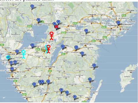
The simulation model has a graphical view (Figure 4): the red stick-figures are electrical engineers while the mechanical ones are cyan. The crosses are corrective tasks while the circles are planned tasks.
Figure 4 – The main view of the simulation model
As the model contains a lot of stochastic variables, a Monte Carlo analysis should be used to estimate the results of the model. In the Monte Carlo analysis the same statistics
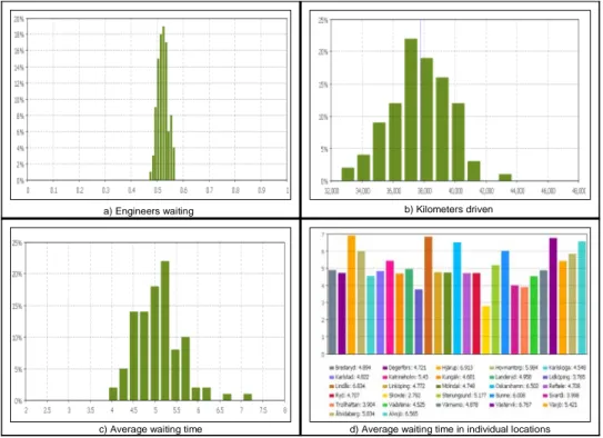
the amount of tasks at individual locations and this statistics indicates the average waiting time for each task. Figure 5a shows an example of one of these statistics and most of the statistics is presented in Table 3. On average the engineers have to wait for work 52% of their time. Only 26% of their total working time is used on the actual value adding time of servicing while 22% is spent of moving between locations. As the engineers have to spend much time traveling between locations, the amount of kilometers driven has a strong impact on the profitability of individual customers. Figure 5b shows the average amount of kilometers driven. The mean value is 37781 kilometers and the amount of standard deviation is 1979 kilometers.
Table 3 – The results for the most important variables.
Variable Mean Standard deviation
Engineers waiting 52.2% 2
Engineers moving 21.6% 1.1
Engineers working 26.2% 1.4
Total kilometers driven 37 781 km 1 979 Corrective waiting time 5.14 hours 0.68
The final statistics, average waiting time overall and at each individual location, mean value depends on a lot of different things. Each individual task’s waiting time does not depend solely on the location but also from the availability of the engineers. This, on the other hand, is impacted by the location of the previous tasks and their length. Also, if a wrong engineer is sent to a corrective task, it requires a lot of time from the engineers. These waiting times are presented in Figures 5c and 5d.
a) Engineers waiting b) Kilometers driven
d) Average waiting time in individual locations c) Average waiting time
Figure 5 – Statistics in the Monte Carlo analysis
As it can be noticed from Figure 5d, the average waiting time on individual locations differs a lot. It should be noted, that even in the town, where the MSP is located, the average waiting time is three hours, despite the fact that the engineers spend 50% of their time waiting for tasks. This can be expected, when the rate of corrective tasks is
relatively high with respect to planned tasks. Figure 5d can also be used to estimate the availability promised to customers.
Discussion and Conclusions
In this research an agent-based decision support system of service related maintenance has been developed. This implies that the real system of interest is modeled and implemented using Agent-Based Modeling and Simulation (ABMS). The resulting simulation model enables the decision-maker to iteratively set parameters, run simulations and evaluate the results. Based on the retrieved information/knowledge the decision-maker can make decisions regarding how to handle the real system. This implies that this type of decision support system fuses information from different sources in a synergistic manner into a situation image that provides effective support for human decision-making.
Some conclusions can be made about the problem domain based on this work. The simulation research findings reveal that response lead time in corrective maintenance differs greatly based on two factors, namely the amount of needed resources, and the travel time. Demand itself is relatively easy to manage since typically only one maintenance resource visit is required when service is actually needed. However, in planned maintenance demand management has a more significant role, since more than one visit on site is typically needed, and the predictability of the number of visits as well as maintenance hours is larger. As the maintenance operator uses a centralized service structure (all resources in one location), considerable amount of time and accumulated costs are tied in traveling to the customer sites. Our simulation experiment shows that management of travel times and costs should receive more attention, and possibly that the centralized service strategy should be modified in the future for a decentralized one.
Additionally an evident problem in successful operation of MSP is the utilization rate of resources vs. customer service level. These parameters are described as a percentage of billed hours vs. total hours and the waiting time spent by customers with regard to rapid, non-planned tasks. By increasing visibility of maintenance tasks and increasing the number of long-term customers, this excluding characteristic can be overcome reducing waiting time for both customer and provider. Increased visibility of incoming tasks could be achieved by: i) increase of accessible information, and increased data capture, ii) change of ratio to favor long-term customers rather than one-stop-shoppers, and iii) increased data gathering for all types of customers, specifically longer term, to enable prediction of maintenance demand.
Based on these results it can be argued that this agent-based decision support system has improved the understanding of problem domain (i.e. maintenance planning) and also generated a basis for decision-making. These results should be generic for other types of service organizations since the problem of achieving a high customer service rate and a high utilization rate is inherently difficult in low-beforehand demand information contexts (e. g. some instances of taxi-operations, ambulance etc). The results of using this type of simulation approach is twofold; i) it is possible to, once the simulation is validated, test the outcome of different settings to find a balance between e. g. customer service rate and utilization rate, the result of new locations on the ratio travel-time and work-time at customers, ii) estimate and motivate the actual value of increased data gathering and information generating in most parts of the work process, e.g. service reports, customer production data etc.
Avenues for further research can be two-fold: (i) the application usage in company management is the most critical (how and where this simulation is useful) and (ii) how
this simulation model could be connected to other decision support systems (e.g. customer relationship management programs or databases).
References
Akkermans, H. and B. Vos (2003). Amplification in service supply chains: an exploratory case study from the telecom industry. Production and Operations Management, 12, 204-223.
Albino, V., N. Carbonara, and I. Giannoccaro (2007). Supply Chain cooperation in industrial districts: A simulation analysis. European Journal of Operational Research, Vol. 177, No. 1, pp. 261-280. Boström, H., Andler, S.F., Brohede, M., Johansson, R., Karlsson, A., van Laere, J., Niklasson, L.,
Nilsson, M., Persson, A. and Ziemke, T., (2007). On the Definition of Information Fusion as a Field of Research,Technical Report HS-IKI-TR-07-006, Informatics Research Centre, University of Skövde.
Cantamessa, M. (1997). Agent-based modelling and management of manufacturing systems. Computers in Industry, Vol. 34, No. 2, pp. 173-186.
Chen, D-N, B. Jeng, W-P Lee, C-H Chuang (2008). An agent-based model for consumer-to-business electronic commerce. Expert Systems with Applications, Vol. 34, No. 1, pp. 469-481. Davidsson, P., L. Henesey, L. Ramstedt, J. Törnquist, and F. Wernstedt (2005). An analysis of
agent-basedapproaches to transport logistics. Transportation Research Part C, Vol. 13, No. 4, pp. 255-271.
Garg, A. and S.G. Deshmukh (2006). Maintenance management: literature review and directions. Journal of Quality Maintenance Engineering, 12, 205-238.
Hilletofth, P., Aslam, T. and Hilmola, O-P. (2009), “Multi-Agent based Supply Chain Management: Case Study of Requisites”, International Journal of Networking and Virtual Organisations, (accepted, forthcoming).
Hilletofth, P., Ujvari, S. and Hilmola, O-.P. (2007), “Information Fusion in Maintenance Planning”, Proceedings of the Swedish Production Symposium, 28-30 August, Göteborg.
Lim, M.K. and Z. Zhang (2003). A multi-agent based manufacturing control strategy for responsive manufacturing. Journal of Materials Processing Technology, Vol. 139, No. 1/3, pp. 379-384. Macal, C.M. and North, M.J. (2006).Tutorial on Agent-based Modeling and Simulation Part 2: how to
Model with Agetns. Proceedings of the 2006 Winter Simulation Conference
Nilsson, F., V. Darley (2006). On complex adaptive systems and agent-based modeling for improving decision-making in manufacturing and logistics settings. International Journal of Operations & Production Management, Vol. 26, No. 12, pp. 1351-1373.
Shen, W., Q. Hao, S. Wang, Y. Li, and H. Ghenniwa (2007). An agent-based service-oriented integration architecture for collaborative intelligent manufacturing. Robotics and Computer-Integrated Manufacturing, Vol. 23, No. 3, pp. 317-325.
Wang, D., S.V. Nagalingam, and G.C.I. Lin (2007). Development of an agent-based Virtual CIM architecture for small to medium manufacturers. Robotics and Computer-Integrated Manufacturing, Vol. 23, No. 1, pp. 1-16.