Pipeline design characteristics of some industrial paste-like slurries

(1)

Pipeline Design Characteristics of

Some Industrial Paste-Like Slurries

G. Addie, M. Carstens, A. Sellgren, R.

Visintainer, and L. Whitclock

(2)

There is a wide variety of industrial pastes or

non-settling slurries pumped in mining,

dredging and reclamation projects as products,

refuse and tails.

Common types / names are:

￫￫￫￫

alumina red mud

￫￫￫￫

phosphate clays

￫￫￫￫

tar sands manure

￫￫￫￫

fine tails

￫￫￫￫

tar sands

￫￫￫￫

(CT) consolidated clays

(3)

Non-settling slurries are formed by a mixture

of fine solid particles and water in which the

solid particles will settle very slowly.

Non-settling slurries flowing in a pipeline

exhibit a nearly uniform distribution of particles

across the flow section and an axisymmetric

velocity distribution and are analyzed as a

pseudo fluid having the specific gravity, Sm.

(4)

The pipeline performance or friction of

these varies dramatically with the type,

its concentration, and the particulars of

the actual slurry making it difficult to

select pumping equipment and to design

associated pipelines.

(5)

The GIW Hydraulic Laboratory in Grovetown

Georgia has tested a number of these

slurries over the last 30 years for various

mining customers.

Where available in the public domain and/or

where permission has been obtained, the

results of those tests are presented in this

paper in a form usable for pipeline and

(6)

Small scale slurry testing can be accomplished in GIW’s 3” closed slurry loop, shown here with a temporary section of 6” piping for a specialty test.

Testing within this type of loop is more economical and requires less

(7)

GIW’s largest closed slurry loop is currently comprised of 20” steel piping (yellow).

Water testing capabilities in excess of 100,000 gal/min can be achieved with the 48” steel pipe loop in conjunction with a 56,400 gallon sealed tank as shown here in blue.

(8)

All permanent GIW test loops are fed by centrifugal slurry pumps.

Specialty testing can be conducted with other pump types as illustrated here by a membrane positive displacement pump.

(9)

The objective in this paper is to present

generalized pipeline loop friction loss results

at various solids concentrations for a variety

of non-settling fine-particle industrial slurries

and briefly discuss the pumpability with

centrifugal slurry pumps.

The pipeline friction loss evaluations are

limited to laminar flows with the focus on

pipeline scaling.

(10)

The pressure gradient, ∆∆∆∆p / ∆∆∆∆x (Pa/m), for flow in a horizontal pipeline is:

j

g

x

p

⋅

ρ

=

∆

where:

j is the friction losses expressed in m of slurry per m of pipe,

ρρρρ is the density of the slurry,

g is the acceleration due to gravity (9.8 m/s2).

(11)

where :

ρρρρo is the density of water

C is the solids concentration by volume calculated by:

where :

ρρρρs is the density of solids

1 S

C

S m

−

=

O S S

S

ρ

=

and:

The slurry density ratio can be expressed as:

3

)

1 S

(

C

1 S

_S O m

=

+

−

ρ

=

2 4

(12)

A force balance for the flowing slurry between two sections a distance ∆x apart relates the pressure gradient, ∆p/∆x and the friction loss gradient, j (eqn 1) to the pipeline wall shear stress,

τ

₀₀₀₀, through the following relationship:

where:

D is the pipeline diameter

4 gjD

4 D

)

x

/

p

(

0

ρ

=

∆

=

τ

5

Pipeline pumping design parameters can be calculated for particular flow rates and velocities with Equation 5 based on friction loss results expressed in terms of shear stresses.

(13)

In all fluids, internal shear stress, τ

₀

, is a

function of the rate of strain.

In uniform flow in a pipe, the rate of strain is

the velocity gradient, du/dr, in which:

u = velocity at a point and

r = the radius

For a Newtonian fluid flowing uniformly in a pipe:

(14)

Equation 6 together with a similar force balance as in Equation 5 for a cylinder with radius r within the flowing fluid in the pipe results after integration and rearrangements (Wilson et al, 1997) in Equation 7 for the wall shear stress:

where:

8V/D is the shear strain at the wall for a Newtonian fluid flowing at velocity V













µ

=

τ

D

V

8

o 7

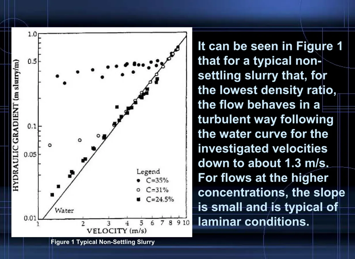
(15)

It can be seen in Figure 1

that for a typical

non-settling slurry that, for

the lowest density ratio,

the flow behaves in a

turbulent way following

the water curve for the

investigated velocities

down to about 1.3 m/s.

For flows at the higher

concentrations, the slope

is small and is typical of

laminar conditions.

(16)

)

D

/

V

8 (ln

d

(ln

d

n

=

τ

0

)

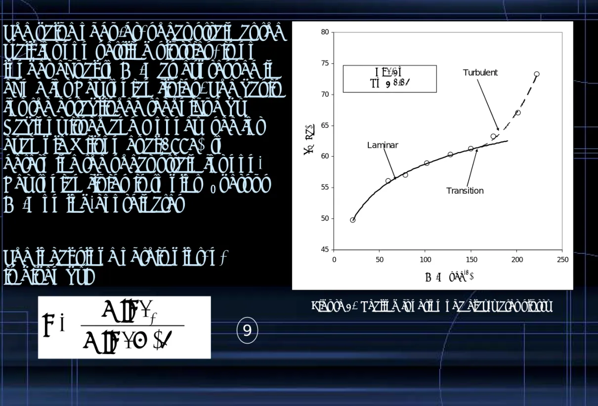
The value of du/dr, shear strain at the wall for non settling slurries, is no longer equal to 8V/D as expressed in eqn 7 for Newtonian fluids. The basis for the established technique by

Rabinowitsch and Mooney (see for example Wilson et al,1997) to

determine the shear strain for non-Newtonian fluids is to plot

τ

₀₀₀₀versus 8V/D on log-coordinates 45 50 55 60 65 70 75 80 0 50 100 150 200 250 8V/D (sec-1) ττττ O (P a ) D=0.2m Sm _≅≅≅≅ 1.13 Turbulent Transition Laminar

Figure 2. Scaling function of a clay-water slurry

The local slope of this plot, n, is given by:

(17)

0.0 0.1 0.2 0.3 0.4 0.5 3 4 5 ln 8V/D lnττττ O n = 0.1087

Figure 3. Graphical determination of n

























+

=

−

D

V

8 n

4 n

3

1 dr

du

As shown in Figure 3, where n is obtained over a considerable span. The rate of strain of a fluid particle adjacent to the pipe wall can then be expressed as:

(18)

Figure 4. Rheogram of clay-water slurry 0 10 20 30 40 50 60 70 80 90 100 0 100 200 300 400 500 Shear Strain ττττ O (P a ) Bingham Fluid

Bingham Coefficient of rigidity η = (0.02 Pas)

Yield Stress τ_yabout 50 Pa

This technique has been applied to the example in Figure 4 with n= 0.11 to obtain the shear strain. The relationship between shear stress and strain rate is known as a rheogram. The rheogram

(19)

From this rheogram, the clay-water slurry closely approximates a so called Bingham fluid with a coefficient of rigidity, η of 0.02 Pas and a yield stress,

τ

_yyyy of about 50 Pa. The Bingham model is

expressed in the following way:













−

η

+

τ

=

τ

_dr

du

y

The power law, or pseudoplastic model, is defined by:

n

dr

du

B

_











−

=

τ

where:

(20)

In order to obtain scaling relationships, evaluated pipeline data for a variety of slurries and concentrations can be empirically fitted to Sm-1 and a constant B and n in an expression similar to eqn 12.

n

0

=

B

(

8 V

/

D

)

τ

(21)

Red Mud 0 50 100 150 200 0 50 100 150 200 250 300 8V/D (sec-1) ττττ 0000 ( P a ) SM = 1.65 SM = 1.55 SM = 1.45

Figure 6. Pipe wall shear stress versus 8V/D for the red mud at various

concentrations Fly Ash 0 50 100 150 200 0 50 100 150 200 250 300 8V/D (sec-1) t 0 ( P a ) SM = 1.58 SM = 1.56 SM = 1.53

Figure 7. Pipe wall shear stress versus 8V/D for fly ash at various concentrations

(22)

Phosphate Clay 0 50 100 150 200 0 50 100 150 200 250 300 8V/D (sec-1) ττττ 0000 (P a ) SM = 1.21 SM = 1.20 SM = 1.18

Figure 8. Pipe wall shear stress versus 8V/D for phosphate clay at various concentrations

Fine Tails & Gypsum

0 10 20 30 40 50 0 50 100 150 200 250 300 8V/D (sec-1) ττττ 0000 (P a ) SM = 1.60 SM = 1.50

Figure 9. Pipe wall shear stress versus 8V/D for fine tails and gypsum at

(23)

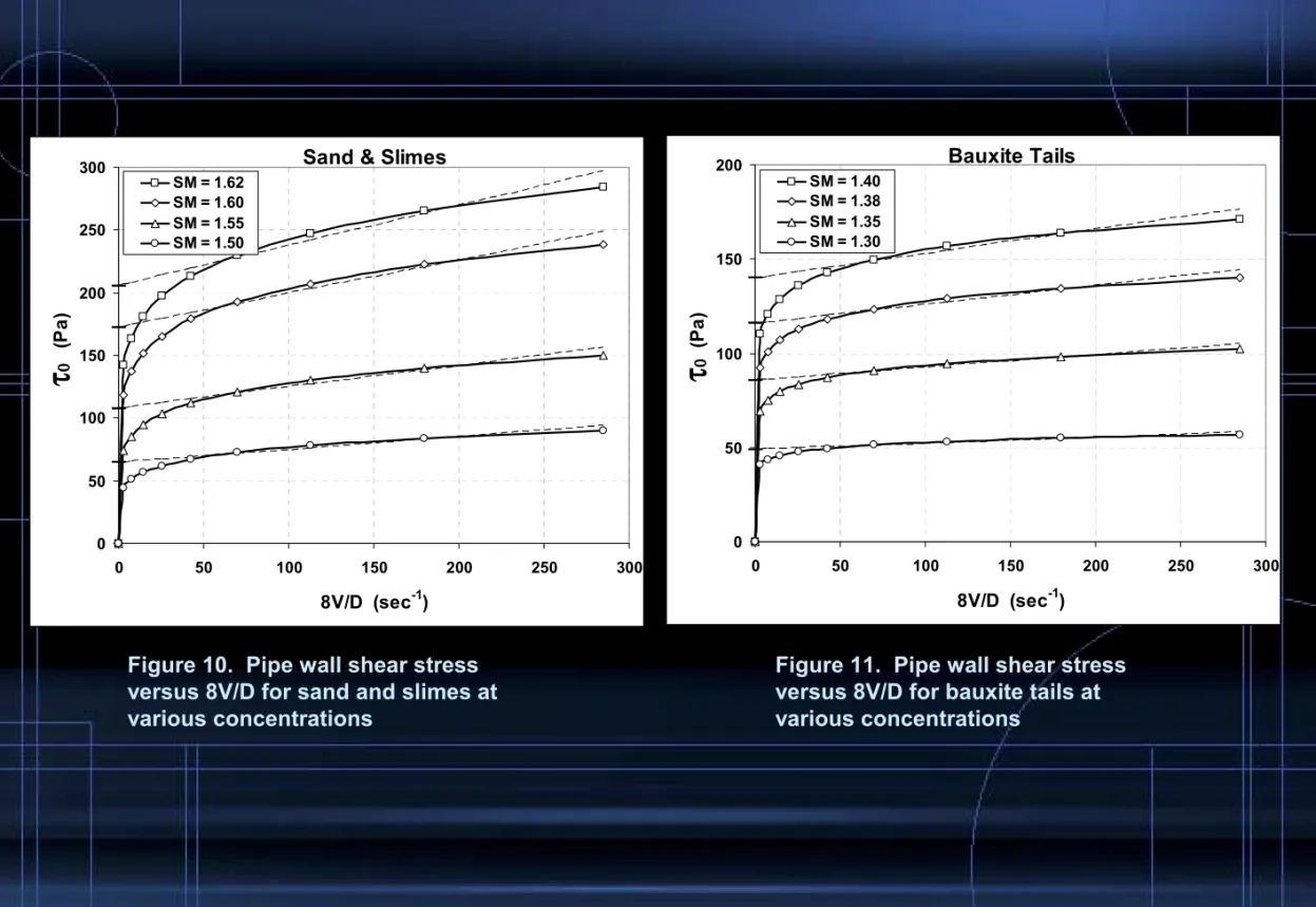
Sand & Slimes 0 50 100 150 200 250 300 0 50 100 150 200 250 300 8V/D (sec-1) ττττ 0000 (P a ) SM = 1.62 SM = 1.60 SM = 1.55 SM = 1.50

Figure 10. Pipe wall shear stress versus 8V/D for sand and slimes at various concentrations Bauxite Tails 0 50 100 150 200 0 50 100 150 200 250 300 8V/D (sec-1) ττττ 0000 (P a ) SM = 1.40 SM = 1.38 SM = 1.35 SM = 1.30

Figure 11. Pipe wall shear stress versus 8V/D for bauxite tails at various concentrations

(24)

Floor

(25)

Trench deposition

(26)

The designer and the owner of a pipeline-pumping

system for a non-settling non-Newtonian slurry

needs to obtain accurate friction loss values for the

full-scale application at a range of operating

conditions. The most reliable way to obtains this is

to scale up experimental results directly with the

scaling parameter 8V/D, based on data in a

pipeline of reasonable size compared to the full

size system.

(27)

A characteristic for all the tested slurries is

the sensitivity of the friction losses to the

solids content with dramatically increased

losses beyond a certain concentration for a

small increase in slurry density.

Variable speed operation for laminar flows

and tight density control are recommended

for centrifugal pumps.

(28)

The yield stress is a key parameter in the design and operation of high density thickening systems. If one parameter was to be

considered as representative of the slurries investigated here, then the effective zero velocity yield stress would be that value that tells most about a given non-settling slurry.

0 50 100 150 200 250 1.0 1.1 1.2 1.3 1.4 1.5 1.6 1.7 SM ττττ Y (P a ) Red Mud Fly Ash Phosphate Clay Fine Tails & Gypsum Sand & Slimes Bauxite Tailings

(29)

Where it is not possible to get enough sample to carry out pipeline tests, a simple test designed by the principle author may be helpful.

As in the picture below a wooden pencil is stuck vertically in a sample in a beaker.

If the pencil falls over, the slurry will likely be pumpable using centrifugal pumps and have shear mess less than 100 Pa.

If it holds firm vertical it will be difficult or impossible to pump.