Active versus
Passive Investing
MASTER THESIS WITHIN: BUSINESS ADMINISTRATION NUMBER OF CREDITS: 15HP
PROGRAMME OF STUDY: MSc International Financial Analysis AUTHOR: Lennart J.P. van Loo & Jonathan Molander
JÖNKÖPING 05 2020
Master Thesis in Business Administration
Title: Active versus Passive Investing, a Comparative Analysis. Authors: Lennart J.P. van Loo and Jonathan Molander
Tutor: Michael Olsson Date: 2020-05-18
Key terms: Active investing, Passive investing, Market timing ability, investor alpha, Fama French 3 factor
Abstract
The increasing popularity of passive investment strategies causes the long-term feasibility of active investing to be questioned more often. Therefore, this research aimed to uncover whether active investors' influence on fund performance is positive and significant enough to offset the cost involved, thereby providing reasoning for active rather than passive investing. A comparative analysis of 211 actively managed funds and 191 market and industry-specific indices is performed. Security selection skills and market timing ability are captured through a model comprising of the Fama French three-factor and the Treynor and Mazuy market timing model. The sample is tested between 2005 and 2020, with 5-year sub-periods.
Over the full period, active and passive returns are found to be nearly indistinguishable. However, active funds seem to excel during bearish periods, where passive funds excel in bullish periods. The standard deviation is higher overall for passive investing. This difference, however, disappears during bearish periods. The security selection skill is barely distinguishable from zero for either strategy. On the other hand, market timing ability is existent for active investors, indicating a positive effect in bearish markets and a negative effect in bullish markets. Additionally, for both investing strategies, more than 90% of the returns are explained by the movements of the general market.
Table of Contents
1 Introduction ... 1 1.1 Problem Statement ...2 2 Literature Review ...3 2.1 Active Investing ...3 2.2 Passive Investing ...52.3 Capital Asset Pricing Model ...7
2.4 Factor Models ...7
2.5 Market Timing ...9
2.6 Time Series Analysis ... 11
2.7 Hypotheses ... 13
3 Data and Methodology ... 14
3.1 Data ... 14 3.2 Descriptive Statistics ... 16 3.3 Methodology ... 23 4 Empirical Results ... 27 4.1 Data Validation ... 27 4.2 Model Selection ... 28 4.3 Regression Results ... 29 4.4 Comparative Analysis ... 30 5 Discussion ... 34 6 Conclusion ... 39 6.1 Limitations ... 41 6.2 Delimitations ... 41 Works Cited ... 42
1 Introduction
The roots of active investing are found over 50 years ago, right after the cold war. What started as a conservative and controlled practice of buying and holding of blue-chip stocks, quickly grew into a booming industry. Active investors attempt to achieve superior returns by uncovering mispriced assets and by timing the market (Han & Hirshleifer, 2012). Uncovering mispriced assets, however, requires firms to gain and interpret information on market developments quickly. To do so, firms started vast research departments to support their traders. Naturally, trading is often done by highly skilled and paid individuals. In addition to the various supporting departments, this quickly accumulated the cost of active investing (Ellis, 2014). However, institutions did not have much choice, as growing competition made the discovery of mispriced assets increasingly harder.
While active investing took off, passive investing commenced in the 1970s, with the creation of the first index fund (Index Industry Association, 2019). Contrary to active investing, passive investing is historically not aimed at market timing and price discovery. Instead, it focusses on purchasing a “basket” of stocks within a specific category. These categories often represent a countries stock market or a particular industry. Once the basked is purchased, the typical strategy is to hold the stocks and prevent interference. By neglecting market timing and price discovery, passive returns have historically been more volatile than active returns.
However, through the development of passive investment strategies, such as factor investing, this gap has decreased over the years. Diversification has always been a central topic within both active and passive investing. However, after the 2008 financial crisis, the desire to diversify grew even further. During this period, factor investing became a trending topic (Roncalli, 2015). The aim of factor investing is to construct a rule-based portfolio that either captures or avoids specific characteristics of securities (Blaise & Quance, 2019). These characteristics are called factors. Though factor investing only gained popularity in the past years, it originates from the Fama and French three-factor model, created in (1992).
1.1 Problem Statement
Passive investing outperformed active investing in terms of the quantity invested for the first time in 2019 (Bloomberg, 2019). Therefore, nearly half of all funds invested globally are still under active management. Yet, in recent years it has become increasingly difficult for active investors to deliver returns superior to the market. While the cost involved in active investing has not diminished, the historic premium for doing so has (Ellis, 2014). Therefore, many investors possibly inefficiently invested large sums of money, fueling an industry run by vastly remunerated individuals, at the cost of the investor’s return on investment.
Attaining an accurate estimation of the cost involved in active and passive investing is hard, especially for a large number of funds. Not only because the cost for investors is often based on multiple variables, but it is also difficult to pinpoint how much firms spent on departments that support traders with research and market analyses.
The value added by the active investor can, however, be measured. Models such as the Fama French five-factor model, and the market timing model by Treynor and Mazuy, attempt to explain the origins of fund returns. The former model, for example, explains returns through factors. The remaining intercept, Jensen’s Alpha, describes the effect of the investor's security selection on the fund's overall performance. The latter model aims to explain an investor’s capability to judge whether the market will go up or down and invest accordingly.
Cost estimation is, therefore, not necessary to judge whether passive investing can outperform active investing. It is possible to argue if active investing has the potential to sustain in the future by uncovering whether the active investor’s influence on the portfolio return is positive and significant. Therefore, under the assumption that active investing is more costly than passive investing, this research aims to uncover whether:
“The influence that active investors have on fund performance is positive and significant enough to offset the cost involved, and thereby provide reasoning for active rather than passive
investing."
In support of the conclusion, several hypotheses will be tested. Prior to introducing these hypotheses in chapter 2.7, the relevant literature will be discussed.
2 Literature Review
In this chapter, a historical overview of active and passive investing is provided. Hereafter, a theoretical background is offered on time series analysis, and the models used for data analysis.
2.1 Active Investing
Active investing is an investment strategy that gained momentum about 55 years ago (Ellis, 2014). It focuses on continually monitoring the money market to exploit profitable opportunities (Han & Hirshleifer, 2012). Right after the second world war and the cold war, the risk aversion was still high. Therefore, active investing was very conservative and under the tight control of the bank and insurance companies' senior management. The primary investment strategy was to buy-and-hold a portfolio that consisted of merely blue-chip stocks. With low trading volumes and long processing times for orders, active investing had a slow start (Ellis, 2014). However, as soon as the early adopters managed to achieve returns superior to the market, it sparked the interest of others, leading to the creation of numerous new firms. The sole purpose of these new firms was to achieve returns superior to those of traditional mutual funds. According to Ellis (2014), excellent opportunities to discover mispriced assets existed during the 1970s and 1980s. This often enabled investment managers to deliver superior returns. Alongside the increased competition technology advanced, and new aids such as the Bloomberg terminal were introduced, making it easier to discover mispriced assets. The increased transparency in asset pricing naturally led to a more efficient market. This made it much harder for an individual investor to discover a mispriced asset, decreasing his chances of delivering superior returns (Fama & Litterman, 2012).
According to Ellis (2014), the management fee banks levied on actively managed assets were historically as low as 0.1%. However, as time passed, fees got higher and higher. The reason given for the price increase is that firms presumed they could simply ask more in fees since a higher fee was associated with higher expected returns. Other types of investors followed suit, and instead of the fees decreasing through increased competition, they rose (Kacperczyk, Van Nieuwerburgh, & Veldkamp, 2014). Wermers (2000) found that the alpha gained from mutual funds before fees and expenses had a positive result. However, after taking the expenses and fees into account, the alpha turned negative, a finding shared by Alexi Savov (2010).
Besides higher management costs, actively managed funds also devote significantly more resources to achieve superior returns, contrary to passive funds. French (2008) compared the cost of active and passive investing throughout 1980-2006. He estimated that the total cost that active investment firms invested in outperforming the market amounted to 101.8 billion USD in 2006. To put this in perspective: "in 2006 investors searching for superior returns in the U.S. stock market consumed more than 330 dollars in resources for every man, woman, and child in the United States” (French K. , 2008). The significance of this amount clearly explains the drive behind the question whether passive investing strategies can ultimately replace active management.
Warren (2020) argues that the diminishing returns and increasing costs of active management do not explain why nearly half of all funds are still being actively managed if doing so is irrational in many cases. However, he states that “decision-making by active investors is impaired by behavioral effects that result in them making an irrational choice. This might be possible, and perhaps the current strong growth in passive investing is a sign of people waking up to past errors” (Warren G. J., 2020). If this is the case, the transition from active to passive is likely to continue.
Ellis (2014) concluded that the funds allocated to passive assets globally grew from 1 to 12.4 percent between 1984 and 2002. Less than a year ago, Bloomberg reported that for the first time in history, more funds are managed passively than active (Bloomberg, 2019). The transition from 1 percent passive management in 1984 to over 50 percent in 2019 signifies a strong trend towards passive investing (Ellis, 2014). Fama analyzed the performance of active U.S. mutual funds for ten years and provided additional reasoning behind the move to passive investing. He pointed out that merely the top three percent of active managers outperformed the market when adjusted for the costs. This means that the highest performing active investors only managed to yield as much as a
2.2 Passive Investing
The introduction of the first index fund in the 1970s marked the beginning of passive investing. Throughout the years, more indices have been created; there are, according to the Index Industry Association, currently over 2.96 million indices worldwide (Index Industry Association, 2019). An example of an index is the OMX-30, which is a capitalization-weighted index of the 30 most traded companies listed in the Swedish stock market.
A passive investing strategy focuses on buying a "basket" of stocks that capture specific characteristics. For example, it can capture an industry, or the entire stock market in a country (Sushko & Turner, 2018). These baskets of stocks are commonly held for an extended period. A passive vehicle, such as an index, is refreshed at a set rate, to include companies that are new to or leaving a market (Strampelli, 2018). Rule-based passive strategies are often refreshed more frequently, as will be further discussed in the coming chapter.
The main downfall of indices is perhaps that they are 'too passive.’ Because of the low refresh rates and straight forward goals, they miss out on many opportunities in the money market, while also not adjusting for the equally opportune risk (Carosa, 2005). Alternative passive investment strategies have been upcoming. These strategies aim to further diversify and lower risk exposure in the case of extreme market movements. Two of the more discussed strategies, factor investing and alternative risk premia, will be discussed.
2.2.1 Factor Investing
The characteristics of securities that help to explain their returns are called factors. Contrary to generic stocks, the value of a factor cannot be directly observed, since factors are constructed based on historical observations. Three different factor types exist: macroeconomic, fundamental, and statistical factors. The macroeconomic factor includes measures such as economic growth, inflation, and interest rates. Fundamental factors, or style factors, are the most widely used today. They focus on capturing stock characteristics, such as valuation ratios and technical indicators. Finally, statistical factors identify characteristics using analytical techniques, such as principal
The need for investments uncorrelated to the market grew after the 2008 global financial crisis. Though factor investing had been around for decades, actively pursuing this strategy required processing large data sets, which was previously impossible. However, due to technological developments in the same period, computing power increased, and alternative (factor) investment strategies became accessible (Roncalli, 2016). One of the strategies that gained ground is alternative risk premia, which is a systematic and rule-based investment strategy. As with factor investing, alternative risk premia utilize factors. The difference between the former and latter is that where factor investing focusses solely on long positions, alternative risk premia combine long and short positions (Goldman Sachs, 2019). An example is the "carry currency" risk premium, which enters a long position in currencies that have high interest rates while shorting currencies with low interest rates (Roncalli, 2017).
Roncalli (2016) identified the lack of regulation as a major shortcoming of alternative risk premia. Currently, no ruling exists on characteristic requirements to brand a security as ‘alternative risk premia’. Reid and van der Zwan (2019), confirm that regulation around the naming of securities poses a potential risk for investors, as securities can be labeled as 'alternative risk premia,' while their structural composition differs greatly, leading to dramatically diverging risk-return profiles.
The most widely used factors are fundamental factors: value, growth, size, and momentum (Bender, Briand, Melas, & Subramanian, 2013). These factors have been studied for decades and are captured by various models, which will be further discussed in the following chapter.
2.3 Capital Asset Pricing Model
The Capital Asset Pricing Model, CAPM hereafter, is an asset pricing theory created by Sharpe and Lintner (1964). CAPM is an equilibrium model that measures the relationship between risk and return; it estimates the cost of capital and helps evaluate portfolio performance (Fama & French, 2004). The model uses a market sensitivity factor to explain the performance of an asset. This measures the movement of an asset in relation to the market. The relation is captured in a beta coefficient (Berk & DeMarzo, 2017). The model states:
𝐸(𝑅𝑖) = 𝑅𝑓 + 𝛽1𝑖(𝐸(𝑅𝑚) − 𝑅𝑓). (1) Where E(Ri) equals the expected return on asset i, the risk-free rate of return is indicated by Rf, and the coefficient representing market sensitivity is denoted as 𝛽𝑚,𝑖.
Michael C. Jensen (1967) evaluated the performance of 115 mutual funds using the CAPM model, after which he proposed an addition to extend the model; Jensen's alpha was created. Jensen's alpha compares an asset's performance with the market's performance while considering both return and risk (Berk & DeMarzo, 2017). Alpha is used to measure an investor’s skill in security selection. A positive alpha indicates a positive impact through security selection, where a negative alpha indicates a negative impact (Elton, Gruber, Brown, & Goetzmann, 2011). Jensen’s alpha, represented by 𝛼𝑖, is introduced to the CAPM model:
𝛼𝑖 = 𝐸(𝑅𝑖) − [𝑅𝑓+ 𝛽1𝑖(𝐸(𝑅𝑚) − 𝑅𝑓)] (2)
2.4 Factor Models
Fama and French (1993) introduced a modified version of the capital asset pricing model. Their model differentiated itself through the introduction of two factors. The size factor, denoted as SMB (Small minus big), captures a corporation's market equity. It is created by differencing a portfolio of small-capitalization stocks with one of large-capitalization stocks, Based on the
The assumption this factor is based on is that firms with a low book-to-market ratio are undervalued, whereas those with a high book-to-market ratio are overvalued (Fama & French, 2012). The addition to the CAPM model is visualized through the SMB and HML variables, with their respective beta coefficient. The Fama and French three-factor model states:
𝐸(𝑅𝑖) − 𝑅𝑓 = 𝛼𝑖 + 𝛽1𝑖(𝐸(𝑅𝑚) − 𝑅𝑓) + 𝛽2𝑖𝑆𝑀𝐵 + 𝛽3𝑖𝐻𝑀𝐿. (3)
Carhart (1997) created a four-factor model by extending the three-factor model with the momentum factor. Carhart recognized the importance of Jagadeesh and Titman’s (1993) one-year momentum anomaly. The momentum factor, denoted as WML (winners minus losers), combines the best-performing stocks in a long portfolio, with the worst-performing stocks in a short portfolio. He performed a comparative analysis of the CAPM, the three-factor model, and the four-factor model. His test included ten different mutual funds from 1963 to 1993. The results indicated that the four-factor model had a higher explanatory factor than the old three-factor model. The momentum variable and its beta coefficient are added to the three-factor model:
𝐸(𝑅𝑖) − 𝑅𝑓 = 𝛼𝑖 + 𝛽1𝑖(𝐸(𝑅𝑚) − 𝑅𝑓) + 𝛽2𝑖𝑆𝑀𝐵 + 𝛽3𝑖𝐻𝑀𝐿 + 𝛽4𝑖𝑊𝑀𝐿. (4)
Fama and French (2014) revised their three-factor model after “evidence provided by Novy-Marx (2013), Titman, Wei, and Xie (2004) that the model was incomplete since it missed a lot of the variation in average returns related to profitability and investments.” Instead of expanding Carhart’s four-factor model, Fama and French ignored the momentum factor and instead used the evidence provided by Novy-Marx to add the profitability and investment factors. In the style of previous factors, the two new factors differentiate the two extremes in their respective category. Robust Minus Weak (RMW) and Conservative Minus Aggressive (CMA), with their corresponding coefficients were added to the three-factor model:
2.5 Market Timing
Treynor and Mazuy (1966) first described market timing ability as the skill to: “increase the portfolio’s exposure to the market or a particular asset class when the manager expects high returns in that asset class and to decrease the portfolio’s exposure when the manager expects low returns.” Treynor and Mazuy created a model to capture market timing skill under the assumption that there should be a relationship between the return of the portfolio and the return of the market if an active investor can predict or forecast stock prices, the model states:
𝐸(𝑅𝑖) − 𝑅𝑓= 𝛼𝑖+ 𝛽1𝑖𝑅𝑚,𝑡 + 𝛽2𝑖𝑅𝑚,𝑡2 + 𝜀𝑖,𝑡 (6)
The alpha generated by security selection is denoted as α𝑖, and the market timing ability factor is
denoted as 𝛽2𝑖. The beta coefficient of the squared market excess return, 𝑅𝑚,𝑡2 , is captured. A
positive coefficient indicates a level of market timing ability is present, that a negative coefficient indicates the investor's attempt resulted in a negative impact on returns (Jagannathan & Korajczyk, 2014). When Treynor and Mazuy tested their model on a sample of 50 funds over ten years, they found only one fund to contain a positive 𝛽2𝑖 at a 5% significance level. Therefore, they had to conclude that there was little evidence to support market timing ability.
Market timing ability was later studied by Henriksson (1984). Rather than using the model by Treynor and Mazuy, he created a new model with Merton. This study divided parametric and nonparametric returns. The difference between which is that parametric requires the fund's returns to be based on a multifactor model or the capital asset pricing model. The model is built up as follows:
𝐸(𝑅𝑖) − 𝑅𝑓= 𝛼𝑖+ 𝛽1𝑖(𝑅𝑀,𝑡− 𝑅𝐹,𝑡 ) + 𝛽2𝑖(𝑅𝑀,𝑡 − 𝑅𝐹,𝑡 ) ⋅ 𝐷 + 𝜀𝑖,𝑡 (7)
The model is reasonably similar to Treynor and Mazuy's model. It does not square the market excess return; instead it multiplies market excess return by a dummy variable, D. The dummy is
Neither researches found evidence that active traders are skilled in market timing. For passive investing, the (Baker & Ricciardi, 2014) technology is not advanced enough to analyze micro/macro economical events and predict stock price movements based hereon. Perhaps artificial intelligence will enable this in the future, until then, only active traders can possess the market ability to time. On the other hand, passive strategies also have advantages over active strategies, such as their ability to eliminate the emotional aspect active traders deal with (Baker & Ricciardi, 2014). Nevertheless, the lack of evidence on the existence of market timing skill is a significant disadvantage for active management. A relevant remark, as pointed out by Baker and Ricciardi (2014), is that both researches focused on mutual fund returns. They suggested hedge funds, which are subject to fewer regulations, can perhaps provide significant evidence of market timing ability. Chen & Liang (2007) studied this and provided significant proof of market timing ability in their sample of 221 hedge funds. They found market timing ability to be especially strong in volatile -and bear markets.
2.6 Time Series Analysis
Fundamental theories on time series analysis are considered. Initially, the choice of regression-model is argued for, after which the trustworthiness of the data and regression outputs are ensured.
2.6.1 Regression Models
Large data sets that contain multiple variables are often tested using a panel data regression (Hsiao, 2007). This type of regression contains observations from different periods, as well as different cross-sectional units. These units describe the independent variables that are tested on the dependent variable. In a panel data regression, both periods and cross-sectional variables are used simultaneously (Gujarati & Porter, 2009). Three different panel data regression models exist. These models differ in how the intermediate effects are handled; the differences will be briefly discussed. The Fixed Effect Model assumes the intercept is equal for all time-series. However, the coefficients for the independent variables all have an identical slope, which is constant over time.
𝐸(𝑅𝑖) − 𝑅𝑓 = 𝛼𝑖+ 𝛽1𝑖 𝑋𝑖,𝑡 + 𝜀𝑖,𝑡 (8)
The Random Effect Model, on the other hand, assumes the intercept consists of a common intercept, plus a random variable that differs between the cross-sections, both of which are time-invariant. The coefficients of the independent variables are considered identical for all time-series and constant over time (Carter Hill, Griffiths, & Lim, 2011).
𝐸(𝑅𝑖) − 𝑅𝑓 = 𝛼1𝑖+ 𝛽2 𝑋𝑖,𝑡 + 𝜀𝑖,𝑡 𝛼1𝑖 = 𝛼1+ 𝜀𝑖
(9)
The Pooled-OLS Model is the simplest model. It 'pools' data from the different time series together, without accounting for different coefficients on the independent variables. The downside of the pooled-OLS model is that it assumes both intercept and all coefficients are equal and time-invariant, which is a dominant assumption.
2.6.2 Model Validation
Stationarity or nonstationarity is an essential element in time-series. Stationary time series are preferred, as they are suitable for forecasting. Nonstationary series are not preferred because they can indicate significant relationships when there are none. This would label the regression as spurious and deem the conclusions taken from it worthless (Carter Hill, Griffiths, & Lim, 2011). A time-series is stationary if both the mean and variance of the random variables are equal within the series, and no autocovariance exists (Gujarati & Porter, 2009)). The Augmented Dickey-Fuller Test can be used to test for unit roots, from which (non)stationarity can be concluded.
To prevent a spurious regression, it is common to prove that the error term variance is constant. If this is not the case, heteroscedasticity occurs, and relevant information can be hidden in the error term. If the error terms are consistent, we have Homoscedasticity (Gujarati & Porter, 2009). Though the Ordinary Least Squares method is built upon the assumption that error terms are normally distributed, and thus homoscedastic, this assumption is often not valid for economic time-series (Brooks, 2008). If the assumptions are violated, the standard error terms in the output can be disturbed. In the case of heteroscedasticity, the regression can be run using the 'robust error term' function, which ensures correct standard errors. The Breusch-Pagan-Godfrey test is used to test for heteroscedasticity.
Finally, it is essential to rule out that the values in the time-series are correlated with a lagged version of themselves, this is called autocorrelation, and it exists in a positive or a negative form. Autocorrelation is another reason for spurious regressions. Proving nonexistence indicates the test results are reliable. The autocorrelation of error terms can be tested using the Durbin Watson test (Gujarati & Porter, 2009).
2.7 Hypotheses
The main research question in this paper reads:
Is the influence that active investors have on fund performance positive and significant enough to offset the cost involved, and thereby provide reasoning for active rather than
passive investing?
In support of the conclusion, argumentation is provided by the following three hypotheses. As mentioned, we will assess the added value of the active investor to the returns of his fund. To uncover whether an active investor's choices in asset allocation leads to above-average returns, we will test whether:
𝐇𝟏: Alpha is indistinguishable from zero.
The results of which will be discussed in chapter 4.3. Additionally, to assess whether an active investor possesses the ability to time the market, and as a result of this achieve above-average returns, we will test whether:
𝐇𝟐: A significant and positive coefficient for market timing ability is nonexistent.
The results of which will also be discussed in chapter 4.3. Finally, regardless of the active investor’s skill, the performance differences between active and passive funds will be assessed by testing if:
𝐇𝟑: Passive and Active investment vehicles achieve indistinguishable performances.
3 Data and Methodology
The coming chapter will describe how the datasets were sourced and what alterations were required to run the regression analyses. Separate panel data are created to represent passive and active investing. Descriptive statistics on both panels will be discussed to share a first impression on the data. The choice between the Fama French three-factor, Carhart four-factor, or the Fama French five-factor model is argued. Finally, this chapter will debate the validity of the data and the model.
3.1 Data
The data in this research consists of monthly price information on active and passive investment vehicles, complemented by data on various factor models. The data was obtained from different sources. G. Haag at Nordnet Bank AB provided data on actively traded funds, which was extracted from a Bloomberg terminal. The Thomson Reuters DataStream repository was used to download price information on passive funds, and the factor data is downloaded from Kenneth French’s data library at the Tuck School of Business. Though the data on active funds dated back to 1999, many of the funds only started operating halfway throughout the sample period or missed data on specific dates. In addition to this, all but the original Fama French three-factor models were introduced after this point in time.
Therefore, the sample was set from January 2005 till January 2020 to capture the most impeccable dataset. This resulted in a 15-year data set; however, previous research has pointed out that effects might be overlooked when analyzing periods that are too long. Bartholdy & Peare (2005) studied this and found that monthly data for periods up to 5 years had the most accurate and relevant results. Therefore, an analysis will not only be performed over the entire sample period but also the following sub-periods:
- Subperiod 1: January 2005 – January 2010 - Subperiod 2: January 2010 – January 2015 - Subperiod 3: January 2015 – January 2020
This way, we can ensure to capture and discuss effects specific to the intermediate periods, such as the 2008 financial crisis.
Focusing on the Eurozone allows us to use area-specific data, which increases the relevance of the results compared to a global focus. For passive funds, applying a geographical focus is straight forward; we opt for indices that solely contain Eurozone stocks. It is challenging to apply the focus for active funds, as a trader in New York can buy a European stock. Therefore, we utilize the Bloomberg geographical focus feature. Bloomberg (2013) states that a fund classified as “U.S." focused, entails that: “the fund invests in equity securities of domestic issuers listed on a nationally recognized securities exchange or traded on the NASDAQ System.” For factor data, the geographical-specific returns are provided by Kenneth French (2020). In addition to this, a more specific market return and risk-free rate data were sourced. The MSCI Europe Index represents the market return, and the EURIBOR monthly rate represents the risk-free rate.
Initially, the passive investment category was supposed to focus on factor investing and alternative risk premia. However, a review of the literature pointed out that funds marketed as alternative risk premia are not necessarily constructed as such. Additionally, many funds were found to dedicate only a percentage of their portfolio to alternative risk premia rather than operating a full alternative risk portfolio (Haag, 2019). Therefore, drawing conclusions on the performance of specific alternative risk premia and factor investing is very hard. Instead, country and industry-specific indexes were chosen as the passive vehicles in this analysis. These indexes can be bought on the stock exchange, just like any other ETF, making them a suitable vehicle to represent passive investments in comparison with actively managed funds.
Nordnet provided global data on 1319 open-end actively managed funds. The scope set on Eurozone funds, with complete data for the entire sample period, left a sample of 211 actively managed funds. An identical amount of passive funds was downloaded from the Thomson Reuters DataStream repository. After filtering, 191 passive funds were found suitable for analysis. A list with the names of the funds included in this analysis is available in Appendix 12 and 13. All data was downloaded as, or converted to, monthly data in U.S. Dollars.
3.2 Descriptive Statistics
The presentation of the descriptive statistics will provide an introduction to the data. Statistics on both the full sample and the relevant sub-periods are discussed. However, some tables that are too vast to present; these will be included in Appendix 1. The implications of the descriptive statistics will be discussed in Chapter 5.
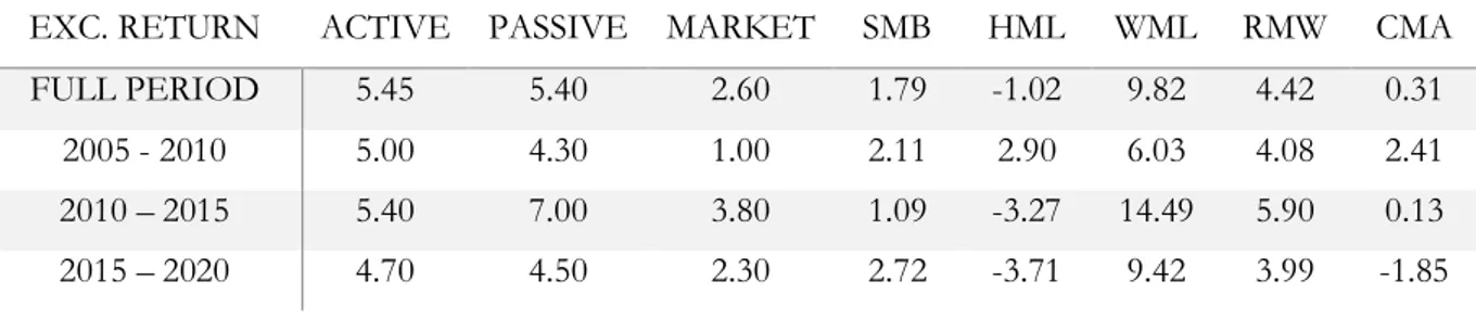
3.2.1 Mean Excess Return
By subtracting the appropriate risk-free rate form raw returns, excess returns are calculated. Table 1 presents the annualized mean excess returns, 'returns' hereafter. When considering the entire sample period, the active and passive portfolios scored a similar return of 5.45 and 5.40 percent. It is important to note that the difference between the better and worse performing investment strategy is the maximum that strategy can cost more in order to truly achieve an edge over the other strategy. Where the returns for the active, passive, and profitability (RMW) were relatively similar, the other variables' returns were significantly lower during the full period. The two most extreme returns are observed for the value factor (HML), which scored the lowest return at -1.02 percent, and the momentum factor (WML), with the highest return, at 9.82 percent, nearly doubling the next highest returning variable.
The difference between active and passive returns is considerably more substantial in the first (two) sub-periods. Though the average first period returns were not affected as much as might have been expected, we observe a higher deviation in returns from Appendix 2. The lowest recorded returns were -6.10 and -32.80 percent for the active and passive panels. During the full period, the minimum returns were merely -2.80 and -7.00 percent. Contrary to the other factors, the mean return of the market was significantly lower, at merely 1.00%. However, the Appendix shows that while the return was lower on average, the highs and lows were less extreme than those of the previously mentioned portfolios.
The momentum factor (WML), is the best performing factor in the first sub-period. The factor managed to continue increasing its lead in the following sub-periods, achieving the highest overall recorded return at 14.49 percent between 2010 and 2015. The momentum factor was not the only variable that scored well during this period, with some exceptions, this sub-period saw the highest returns in general. In the same period, passive investing outperformed active investing, delivering 7.00 percent, whereas active portfolios only managed 5.40 percent, respectively.
This lead was lost during the final sub-period, where a collective decrease in returns is observed. However, the decrease is not as significant as the first sub-period, and the highs and lows are less extreme than in the other sub-periods.
There are some additional significant findings from Table 1. While the first sub-period was, on average, the worst-performing period, the value factor (HML) excelled at this time. Where the other variables thrived in later periods, the value factor scored highly negative returns. On the contrary, the size factor (SMB), had its worst period from 2010 to 2015, which is where all other factors performed best. Finally, the investment factor (CMA), also presented a different development throughout the sub-periods. Where the general pattern was low, high, low, the investment factor was the only factor to boast a constant, gradually decreasing return pattern.
Table 1: Annualized Excess Return
EXC. RETURN ACTIVE PASSIVE MARKET SMB HML WML RMW CMA
FULL PERIOD 5.45 5.40 2.60 1.79 -1.02 9.82 4.42 0.31
2005 - 2010 5.00 4.30 1.00 2.11 2.90 6.03 4.08 2.41
2010 – 2015 5.40 7.00 3.80 1.09 -3.27 14.49 5.90 0.13
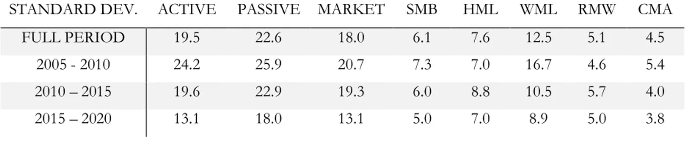
3.2.2 Standard Deviation
The standard deviation uncovers how returns are positioned around the mean. Higher standard deviations indicate that the returns tend to be placed further away from the mean, where lower standard deviations have returns positioned closer to the mean. Table 2 presents the standard deviation of the tested variables.
By far, the highest standard deviation is achieved by active and passively managed funds during the first sub-period, at 24.30 and 25.90 percent. The market portfolio and momentum factor followed suit with a slightly lower deviation. However, most of the other factors had a significantly lower standard deviation than the previously mentioned variables. Over time, the passive and market portfolio decrease their standard deviation at the same rate. Active traders, however, manage to decrease their standard deviation by nearly 50 percent, to 13.10 percent, identical to the market portfolio. This is a significantly more substantial decrease than the passive funds realized, which decreased to 18.00 percent. For most other factors, a slight decrease, or a stable standard deviation was observed over the subsequent periods.
Remarkably, the standard deviation for the momentum factor (WML) is by far lower than the active, passive, market portfolio, while the excess return for this factor was high. An identical observation, with a smaller difference, is observed for the profitability factor.
Table 2: Standard Deviation
STANDARD DEV. ACTIVE PASSIVE MARKET SMB HML WML RMW CMA
FULL PERIOD 19.5 22.6 18.0 6.1 7.6 12.5 5.1 4.5
2005 - 2010 24.2 25.9 20.7 7.3 7.0 16.7 4.6 5.4
2010 – 2015 19.6 22.9 19.3 6.0 8.8 10.5 5.7 4.0
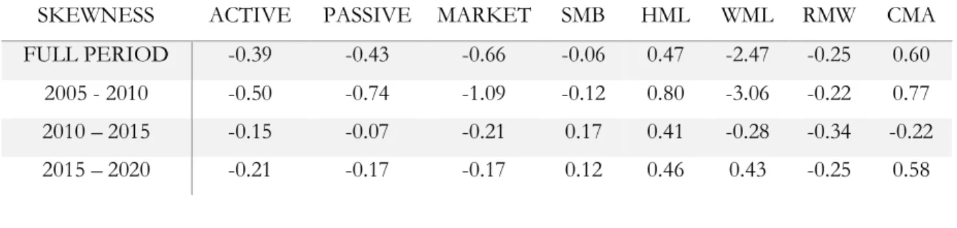
3.2.3 Skewness
Skewness indicates whether a distribution is positioned leftwards or rightwards of the mean, as presented in Table 3. Over the entire period, the active and passive portfolios indicated a negative skewness of -0.39 and -0.43, respectively. Negative results indicate a leftward skewed distribution, which results in a mean lower than the median. The same observation is made for all factors except the value and investment factor, which were highly positive. From the development in the sub-periods, we get a better understanding of how the numbers of the full sample period are built up. In the first sub-period, the most extremely skewed distributions are observed. The market and momentum factors indicate the most negatively skewed distributions.
Meanwhile, the value and investment factors are the only factors with positive skewness. In the two following sub-periods, all factors move closer to 0, and thus a normal distribution. Extreme increases are seen for the market and momentum factor. It is interesting to note that the size, momentum, and investment factor even switch signs during the sub-periods. Overall the distributions grow closer to normal over time; however, the active and passive portfolios both drifts slightly further away again in the last sub-period, with skewness of -0.21 and -0.17.
Table 3: Skewness
SKEWNESS ACTIVE PASSIVE MARKET SMB HML WML RMW CMA
FULL PERIOD -0.39 -0.43 -0.66 -0.06 0.47 -2.47 -0.25 0.60
2005 - 2010 -0.50 -0.74 -1.09 -0.12 0.80 -3.06 -0.22 0.77
2010 – 2015 -0.15 -0.07 -0.21 0.17 0.41 -0.28 -0.34 -0.22
3.2.4 Kurtosis
Kurtosis indicates how sharp the peak in a distribution of returns is. Over the entire period, a broad range in kurtoses are observed, from 0.12 to 17.45, while the median is only 1.89. Most factors have a kurtosis close to the median, only the size, value, and profitability factor score lower at 0.12, 0.81, and 0.49, respectively. The low kurtosis levels, in general, indicate thinner tails than those of a normal distribution. When observing the sub-periods, it is very apparent that there are extreme changes in the kurtosis levels compared to the overall period. As seen in Table 4, the active, passive, and market portfolio all have a positive and relatively high kurtosis of 2.02, 2.83, and 2.72 in the first sub-period, after which all drastically decrease. For some, such as the market factor, kurtosis even becomes negative. The most drastic decrease is seen in the momentum factor, which starts at 15.56 and ends at 0.46.
Table 4: Kurtosis
KURTOSIS ACTIVE PASSIVE MARKET SMB HML WML RMW CMA
FULL PERIOD 2.30 1.99 1.79 0.12 0.81 17.45 0.49 2.04
2005 - 2010 2.02 2.83 2.72 -0.13 3.89 15.56 3.46 2.37
2010 – 2015 0.91 0.21 0.11 0.26 -0.70 1.97 -0.67 -0.32
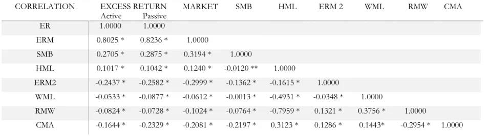
3.2.5 Correlation
Correlation indicates if there is a relationship between two variables. The table for active and passive investing was merged since all variables except for the excess returns are equal. Table 5 represents the correlation matrix for the full sample period, the significance levels are indicated with asterixis. The correlation tables for the sub-periods are accessible in Appendix 1.
Over the full period, we observe similar correlations between active and passive funds and the independent variables. All independent variables show high significance levels for both the active and passive portfolios. The market excess return, size, and value factor show a positive correlation to the two portfolios. The remaining independent variables show a negative correlation. From the negatively correlated variables, the market timing and investment variable show the most significant negative correlation towards active and passive portfolios, at -0.2582 and -0.2437 for market timing, and -0.2329 and -0.1644 for the investment factor. The size and value factors both indicated a low but positive correlation with the portfolios. The market excess return has the highest correlation, with 0.8236 for active, and 0.8025 for passive.
From Appendix 1, we observe that the correlation between the independent variables and the two portfolios is relatively in the first sub-period, compared to the following sub-periods1. All independent variables are highly significant in the first period. In the second and third sub-periods, all variables are significant, except for the investment variable in the second, which is insignificantly correlated. The correlation for the market return is similar in the first and second sub-periods, ranging between 0.8157 and 0.8501. A decrease is visible in the third sub-period, towards 0.7396 and 0.7208 for the active and passive portfolios. From the sub-periods, it is interesting to note that nearly all variables change from positive to negative, or vice versa.
Table 5: Correlation
(* = significant at one percent. ** = significant at five percent.)
CORRELATION EXCESS RETURN
Active Passive MARKET SMB HML ERM 2 WML RMW CMA
ER 1.0000 1.0000 ERM 0.8025 * 0.8236 * 1.0000 SMB 0.2705 * 0.2875 * 0.3194 * 1.0000 HML 0.1017 * 0.1042 * 0.1240 * -0.0120 ** 1.0000 ERM2 -0.2437 * -0.2582 * -0.2999 * -0.1362 * -0.1615 * 1.0000 WML -0.0533 * -0.0877 * -0.0612 * -0.0013 * -0.4931 * -0.0348 * 1.0000 RMW -0.0824 * -0.0728 * -0.1024 * -0.0764 * -0.7959 * 0.1321 * 0.3756 * 1.0000 CMA -0.1644 * -0.2329 * -0.2081 * -0.2197 * 0.3123 * 0.1286 * 0.1443* -0.2954 * 1.0000
3.3 Methodology
The sample consists of 211 actively managed funds, 191 indices, and Fama French European factor data. This data is considered between January 2005 and January 2020, while also taking the three intermediate, five-year sub-periods into account. All data is downloaded as, or converted to monthly prices in US-dollar, after which returns are calculated using:
𝑅𝑖𝑡 = 𝑅𝑖𝑡− 𝑅𝑖𝑡−1
𝑅𝑖𝑡−1 (11)
Apart from the regression, a comparison of active and passive performance over the past 15 years is conducted. Herefore, we consider key performance measures such as returns, standard deviation, expected shortfall, Sharpe ratio, and Sortino ratio. These statistics will enable a comparison between the two investment types while disregarding factors like cost and value-added by an investor.
3.3.1 Regression Model
This research uses the 'Panel Least Squares' approach because it allows the analysis of over 200 funds simultaneously. An Individual ‘Ordinary Least Squares’ regression would have entitled us to conclude how many, and which funds achieve a positive alpha, however, for this research that would not contribute to the outcome. Being able to conclude whether alpha exists, on average, in the sample, is sufficient to argue whether active -or passively managed funds possess an advantage over one another.
The original Fama French 3 factor model, as well as the four-factor extension created by Carhart, and the five-factor model by Fama French, will be considered. Though the older three-factor model has been used more widely, recent research promotes the relevance of the newer factors. In 2012, research by Connor, Hagmann, & Linton pointed out that the two newest factors are at least as important, if not more important, than the original three factors when explaining returns (Connor, Hagmann, & Linton, 2012). The most suitable model will be chosen based on the
The three regression models considered in this research are as presented below. In the coming paragraphs, the variables in these regression models will be further explained.
𝐸(𝑅𝑖) − 𝑅𝑓 = 𝛼1+ 𝛽1 (𝐸(𝑅𝑚) − 𝑅𝑓) + 𝛽2,𝑖𝑆𝑀𝐵 + 𝛽3,𝑖𝐻𝑀𝐿+ 𝛽4,𝑖𝑅𝑚,𝑡2 (12) 𝐸(𝑅𝑖) − 𝑅𝑓 = 𝛼1+ 𝛽1 (𝐸(𝑅𝑚) − 𝑅𝑓) + 𝛽2,𝑖𝑆𝑀𝐵 + 𝛽3,𝑖𝐻𝑀𝐿 + 𝛽4,𝑖𝑊𝑀𝐿 + 𝛽5,𝑖𝑅𝑚,𝑡2 (13) 𝐸(𝑅𝑖) − 𝑅𝑓 = 𝛼1+ 𝛽1 (𝐸(𝑅𝑚) − 𝑅𝑓) + 𝛽2,𝑖𝑆𝑀𝐵 + 𝛽3,𝑖𝐻𝑀𝐿 + 𝛽4,𝑖𝑅𝑀𝑊 + 𝛽5,𝑖𝐶𝑀𝐴 + 𝛽6,𝑖𝑅𝑚,𝑡2 (14) Jensen’s Alpha
Jensen’s Alpha, Denoted as "𝛼," is perhaps the most widely used approach to measure the value managers added to the performance of their portfolio (Bunnenberg, Rohleder, Scholz, & Wilkens, 2018). The measure is included in many financial and economic models, such as the Capital Asset Pricing Method, and all factor models considered in this research. These factor models try to explain returns through factors such as size or value. If, after accounting for the factors, a positive and significant alpha is found, it indicates that the manager's contribution to asset selection had a positive impact on the portfolio's return.
Market Return and Risk-Free Rate
The market return and risk-free rate denoted as 𝑅𝑚, and 𝑅𝑓, are two crucial variables. Through
the use of geographically relevant rates, increased significance is expected.
Therefore, the MSCI Europe index represents the market return. This index "Covers more than 2,700 securities across large, mid, small and micro-cap size segments and across style and sector segments in 15 developed markets” (MSCI, 2020). As the index covers a broad spectrum of the European stock market, it is an excellent index to represent the market return.
The risk-free rate is represented by the one-month Euro Interbank Offered Rate, Euribor. Within the European market, the Euribor is considered to be the foremost used reference rate (Euribor, 2020).
Fama French Factors
Kenneth French provides factor data. The three-factor model's size and value factors are denoted as 𝛽2,𝑖𝑆𝑀𝐵, and 𝛽3,𝑖𝐻𝑀𝐿. The size factor represents the difference in small and large-cap stocks
returns, hence its antonym SMB, Small Minus Big. The value factor, denoted as High Minus Low, represents the difference between growth and value stocks, measured by their book to market ratio (Bodie, Kane, & Marcus, 2018). Carhart later introduced the momentum factor, denoted as 𝛽4,𝑖𝑊𝑀𝐿, Winners Minus Losers. This factor utilizes the difference between winning and losing stock over the past 12 months. Fama and French later reworked their original model in 2014. However, instead of including Carhart's momentum factor, they opted to introduce the profitability and investment factors (Fama & French, 2014). These factors are denoted as 𝛽4,𝑖𝑅𝑀𝑊, and 𝛽5,𝑖CMA, for Robust Minus Weak and Conservative Minus Aggressive. Each of
which takes the difference between the best and worst-performing stocks in this category. (French K. , Data Library, 2020)
Market Timing Ability
The market timing ability factor by Treynor and Mazuy, denoted as 𝛽4,𝑖𝑅𝑚,𝑡2 , is incorporated into the Fama French model. We create a new variable, based on the MSCI Europe returns, by squaring them. The presence of market timing ability can be concluded if the coefficient (𝛽4,𝑖) is significant and positive.
3.3.2 Model Validation
The models are tested for several potential issues, to ensure that regression outputs are reliable. Initially, arguments for the choice between a fixed effect, random effect, or pooled-OLS regression model will be presented. After this, we will provide evidence that our regression
is not spurious.
A Hausman test is performed to uncover whether the random or fixed effect model provides the best fit to the data. This test checks for correlation between the independent variables and the error term. If the correlation is nonexistent, both the random and fixed effect models will produce
A Breusch Pagan test is used to differentiate between the random-effect and the Pooled-OLS model. As mentioned in the literature review, the Pooled OLS model assumes all time-series have an identical intercept. This would mean that there is no variance in the random effect of the random effect model's intercept. Significant test results indicate that the Random Effect Model is required; otherwise a Pooled-OLS model is sufficient. Additionally, the Breusch Pagan test can also be used to test for heteroscedasticity. A significant Chi-square from the test will conclude heteroscedasticity, where an insignificant result indicates Homoscedasticity. In the case of heteroscedasticity, robust standard errors are calculated.
Stationarity is an essential factor to validate the data in a time series analysis. A popular test to conclude stationarity is the Dickey-Fuller Test, which tests for unit roots. In this research, testing is performed using the augmented panel version of the Dickey-Fuller Test, as this allows for testing models of unknown order (Zivot & Wang, 2006).
Finally, data validity is ensured through the nonexistence of autocorrelation using the Durbin Watson test for autocorrelation. The output is more complicated than other types of tests. The analysis presents a number in the range of 0 to 4. Results close to 0 and 4 indicate positive and negative autocorrelation, while a number close to 2 indicates no signs of autocorrelation. A complicating factor is the inconclusive area in the outputs, the borders of which tell one exactly how close to 2 their Durbin Watson statistic has to be in order to conclude nonexistence of autocorrelation. These critical values depend on the number of variables and the sample size of the regression.
4 Empirical Results
This chapter will present the findings and all results that are necessary for the discussion chapter that follows.
4.1 Data Validation
Initially, we tested to find the best fitting regression model for our data, after which several tests will validate the data quality and trustworthiness of the regression outputs.
The Hausman test indicates whether the fixed effect model or the random effect model gives more consistent results. For the passive and active funds, the Hausman test results were highly insignificant, with a probability of 1.0000. The test outputs are included in Appendix 3 the test stated: "Cross-section test variance is invalid. Hausman statistic set to zero.". This message occurs because the test is unable to identify variations between the random and fixed effect cross-section effects. With a probability of 1.0000, we cannot reject the 𝐻0. Therefore, both the fixed effect and
random effect model can be used. The Breusch Pagan test points out whether pooled-OLS provides more consistent results.
The Breusch-Pagan test delivers sub-hypotheses for the time and cross-section effects. All results were highly significant at 0.0000, therefore, the null hypothesis can successfully be rejected. The test results are included in Appendix 10. These results indicate that the random effect model is preferred over the pooled-OLS model.
Apart from the test results, the random effect model would also be found most relevant, as it allows for an individual intercept (alpha). It makes sense to capture individual alphas in each fund, as identical alphas would make it hard to compete on the market. Additionally, the significant test results from the Breusch-Pagan test also conclude the existence of heteroskedasticity, which can cause a disturbance of the error terms. To prevent distorted error terms, we ensured robust standard errors through the ‘white period’ coefficient covariance method is in the regression.
4.2 Model Selection
As mentioned in the literature review, several variations of the Fama French factor model have been released in the past years. Though other research has pointed out the relevance of the later additions to the original three-factor model, we have tested all three models to find out which one is the best fit to our data. The characteristics considered in this analysis are the adjusted R-squared and the probability values of the independent variables. The probability values indicate how significant the independent variables are in explaining the dependent variable. In addition, the adjusted R-squared gives an overall score on how well the model describes the dependent variable. The normal squared will always slightly increase when new variables are added. The adjusted R-squared, however, shrinks when the newly introduced value does not explain the dependent variable better than the model without this new variable. Table 6 presents the adjusted R-squared results for each model computed using the random effect model.
ADJUSTED R-SQUARED ACTIVE ∆% PASSIVE ∆%
FAMA FRENCH 3 FACTOR + MT1 0.68055 - 0.64458 -
CARHART 4 FACTOR + MT 0.68464 + 0.00409 0.64464 + 0.00006
FAMA FRENCH 5 FACTOR + MT 0.68302 - 0.00162 0.64459 - 0.00005
Table 6: Adjusted R-squared
By introducing the 4th factor, the adjusted R-squared grows. However, when evaluating the five-factor model, the adjusted R-squared shrinks. Though the four-five-factor model has a higher overall adjusted R-squared, the increase in adjusted R-squared is only by 0.002075 percent. Therefore, we conclude that the introduction of the fourth factor does not result in a significantly better model. To prevent the omitted variable bias, we opt to stick to the Fama French 3 Factor model, complemented by the market timing ability factor.
An adjusted R-squared statistic of 0.68055 and 0.64458 can be perceived as a good fit. Comparable research by Orback and Nordlinder (2019) found values between 0.4931 and 0.5541.
4.3 Regression Results
A random effect panel data regression is run on the Fama French 3 factor model with a market timing variable. All variables were sourced with a focus on the Eurozone. The regression results are included below:
Table 7: Active Regression Outputs (* = significant at one percent. ** = significant at five percent. “-“ = Insignificant)
Table 8: Passive Regression Outputs (* = significant at one percent. ** = significant at five percent. *** = significant at ten percent. “-“ = Insignificant)
Prior to presenting the results, we consider the Durbin Watson statistic. This statistic only becomes available once a regression has run. The active funds' Durbin Watson statistic of 2.0117, as well as the passive funds' statistic of 1.9588, fall within the critical values. This means we can reject the 𝐻0 and conclude the nonexistence of autocorrelation.
The alpha coefficient in either passive and active panel is highly significant, with a probability of 0.0000. However, the coefficients read 0.0028 for active funds and 0.0023 for passive funds, which is barely distinguishable from zero. Regardless of the size of the coefficient, it is interesting to see
ACTIVE ADJ. R2 ALPHA ERM SMB HML ERM 2
FULL PERIOD 0.6806 0.0028* 0.9135* 0.0894* - -0.1238*
2005 – 2010 0.6988 0.0021* 1.0124* 0.1352* 0.0299** 0.2559*
2010 – 2015 0.7235 0.0023* 0.9022* -0.0662* - -0.2037*
2015 - 2020 0.5507 0.0028* 0.7676* -0.0528* -0.0671* -
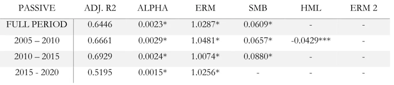
PASSIVE ADJ. R2 ALPHA ERM SMB HML ERM 2
FULL PERIOD 0.6446 0.0023* 1.0287* 0.0609* - -
2005 – 2010 0.6661 0.0029* 1.0481* 0.0657* -0.0429*** -
2010 – 2015 0.6929 0.0024* 1.0074* 0.0880* - -
For both fund types, excess market return is highly significant. The coefficient reads 0.9135 and 1.0287, for active and passive funds. Throughout the sub-periods, excess market return’s coefficient has remained stable slightly above 1 for passive investing. Active investing, on the other hand, showed a steady decrease to 0.7676 in the final period.
Though its coefficients are lower than market excess return, the size factor is highly significant, with a probability of 0.0000. The coefficients are 0.0894 and 0.0609 for active and passive funds, respectively. For the size factor, again, there is an inverse growth pattern between the active and passive funds. Where the coefficient grows for passive funds, it decreases for active funds.
For both active and passive funds, the value factor was highly insignificant, with probabilities of 0.4613 for active, and 0.4023 for passive funds. During testing with the four and five-factor model, this factor's probability shrank slightly. However, it never became significant, not even at the 10% level. From sub-period testing, the factor appears to be significant only for the last sub-period, 2015-2020, for active funds. Here, the value factor had a negative coefficient of -0.0671.
With a probability of 0.0004, market timing is found to be highly significant in actively managed funds, with a negative coefficient of -0.1238 on average. However, a strong trend is found in the sub-periods. Where the first period posted a positive effect of 0.2559, this effect steadily declined into negative -0.3100 in the last subperiod. The coefficient is found highly insignificant for passive funds, with a probability of 0.5063, this pattern of insignificance continues throughout all sub-periods.
4.4 Comparative Analysis
The focus of this analysis lies in several financial ratios that provide a broader view of the active and passive fund performance. Two variables that belong to the comparative analysis are the mean excess return and the standard deviation, which have already been presented in Chapter 3.2. These topics will not be repeated, but their repercussions will be reflected in the discussion.
4.4.1 Sharpe ratio
The Sharpe ratio provides a clear insight into the trade-off between the risk and return of a given asset. A higher Sharpe ratio results in an investor being rewarded with additional return for every bit of extra risk he takes on (Dowd, 2000).
Over the full period, a ratio of 0.28 and 0.24 is observed for active and passive investing. With lower minimums and higher maximums, active investing appears to offer better risk-return payoff. The sub-periods offer more detailed insight. The global financial crisis in 2008, captured in the first sub-period, showcases the smallest gap between active and passive Sharpe ratio. Though the averages are very similar, significant differences are observed when considering the minimum and maximum values. Active investing indicated that the lowest Sharpe ratio was -0.55 during the crisis, just under twice as low as the average. On the other hand, passive investing scored -2.22 for the lowest Sharpe ratio, more than four times as low as the average ratio. On the up-side, passive indices also scored a higher maximum Sharpe ratio than actively managed portfolios. From these results, we can conclude that the 'passive' nature of indices causes them to be more vulnerable to bearish market conditions. On the contrary, the passive nature of indices is not all bad, as we have seen in the descriptive statistics. Though the deviation is larger, the average return exceeds that of actively managed funds. During the periods following the crisis, an increase in the Sharpe ratio is seen for both investing strategies. Whereas the maximum observed ratio is relatively stable for passive investing, a vast increase is seen for active investing.
SHARPE RATIO Active Passive AVERAGE Active Passive MINIMUM Active Passive MAXIMUM Active Passive MEDIAN
FULL PERIOD 0.28 0.24 -0.28 -0.50 0.47 0.37 0.29 0.27
2005 – 2010 0.20 0.17 -0.55 -2.22 0.55 0.64 0.18 0.17
2010 – 2015 0.28 0.31 -0.77 -0.92 0.77 0.53 0.30 0.38
4.4.2 Sortino ratio
Where the Sharpe Ratio takes both positive and negative returns into account, the Sortino ratio only considers the negative returns. Therefore, this metric is included to give a clearer image of the downside risk taken, compared to the returns achieved. Over the full period, results similar to the Sharpe ratio are observed. With 0.37, the actively managed funds score better than the passive indices, which score 0.33, a small difference. During the crisis period, a more significant difference between active and passive is observed than in the Sharpe ratio, indicating that active investors are better at protecting their downside risk during bearish periods. Additionally, extreme minimums and maximums are observed for passive investing. This indicates that besides very bad indices, some indices outperformed the average active investor during a crisis period. A positive growth pattern developed after the crisis. Contrary to the Sharpe ratio, we observe lower minimum scores accompanied by higher maximum scores. This indicates that not all active investors were able to decrease their exposure to downside risk after the crisis, as their exposure worsened.
SORTINO RATIO Active Passive AVERAGE Active Passive MINIMUM Active PassiveMAXIMUM Active PassiveMEDIAN
FULL PERIOD 0.37 0.33 -0.41 -0.72 0.63 0.55 0.37 0.35
2005 – 2010 0.26 0.20 -0.75 -2.95 0.69 0.72 0.22 0.21
2010 – 2015 0.40 0.49 -1.31 -1.38 0.85 0.95 0.44 0.60
2015 - 2020 0.56 0.40 -1.03 -1.71 1.58 0.81 0.56 0.41
4.4.3 Expected Shortfall
The expected shortfall, also known as conditional value at risk, measures the expected loss in the worst-case scenario. It quantifies the loss that occurs if the threshold of the value at risk is broken. In the worst-case scenario, the average expected loss for the active and passive portfolios is -17 and -19 percent. The minimum and maximum values are close to the average, which indicates the expected losses are similar across the panel. Throughout the sub-periods, a clear downward trend is visible. Both active and passive strategies have their worst expected shortfall in the first sub-period, after which they follow a similar trend upwards. Active investing has a slight edge over passive in the final sub-period. Active investing also has more favorable results for maximum values, though the lead is barely distinguishable. A different pattern is found for the minimum values. Where the active investors seem to decrease their worst expected shortfall, the passive score barely changes; after a slight decrease, it remains stable at -0.24. Over all periods and measures, the active funds have a slight edge over the passive indices.
EXP SHORTFALL Active Passive AVERAGE Active Passive MINIMUM Active PassiveMAXIMUM Active PassiveMEDIAN
FULL PERIOD -0.17 -0.19 -0.28 -0.33 -0.08 -0.10 -0.18 -0.19
2005 – 2010 -0.16 -0.17 -0.27 -0.29 -0.07 -0.10 -0.17 -0.18
2010 – 2015 -0.12 -0.13 -0.19 -0.24 -0.05 -0.07 -0.13 -0.13
5 Discussion
This chapter will discuss the findings in this research. Initially, the choices made around the regression model are discussed. Hereafter, the outcomes of the factors can be discussed. At first, the factors that are not related to a hypothesis will be discussed. Afterward, the remaining factors will be discussed in the order the hypotheses are presented in chapter 2.7.
Regression Model
Literature by Linton et. all concluded that the additional factors introduced in the Carhart four-factor and Fama French five-four-factor model explained significantly more than the original Fama French three-factor. However, our research found the opposite to be true. Though the Adjusted R-squared, which measures the fit of the model used, was higher, the four and five-factor model only explained +0.0021% more and -0.0008% less than the original Fama French three-factor model. This change is so small that we avoided adding more variables to our regression to prevent overfitting the model. The difference between this and Linton's research rests on the fact that the sample sizes differ tremendously. Where Linton researched a sample of yearly data between 1970 and 2007, this research considered monthly data from 2005 till 2020. This makes that the sample considered in their research is significantly larger, which could influence the fit of the model. Still, in this research, it did not explain significantly more enough to include the additional factors in the model.
Factors
The two rule-based factors in this regression are the size and value factor. Unfortunately, the value factor was highly insignificant in all but two regressions. The reason here fore should be discussed. Both the size and value factors are factors that track the co-movements of stocks that share characteristics. However, it is essential to note that the characteristics determine the significance, not their co-movements (Chung, Johnson , & Schill, 2006). Therefore, the insignificance is likely caused by a weak correlation with the book-to-market ratio. This ratio is possibly distorted because funds and indices are used rather than individual stocks, where the characteristics would be more specific.
Naturally, a positive coefficient for a size factor indicates dominance by large-cap stocks. However, Chen and Basset (2014) indicated that when large-cap stocks dominate the market factor, a positive