One Tree to Explain Them All
Ulf Johansson
School of Business and Informatics University of Borås
Sweden
Email: ulf.johansson@hb.se
Cecilia Sönströd
School of Business and Informatics University of Borås
Sweden
Email: cecilia.sonstrod@hb.se
Tuve Löfström
School of Business and Informatics University of Borås
Sweden
Email: tuve.lofstrom@hb.se
Abstract—Random forest is an often used ensemble technique, renowned for its high predictive performance. Random forests models are, however, due to their sheer complexity inherently opaque, making human interpretation and analysis impossible. This paper presents a method of approximating the random forest with just one decision tree. The approach uses oracle coaching, a recently suggested technique where a weaker but transparent model is generated using combinations of regular training data and test data initially labeled by a strong classifier, called the oracle. In this study, the random forest plays the part of the oracle, while the transparent models are decision trees generated by either the standard tree inducer J48, or by evolving genetic programs. Evaluation on 30 data sets from the UCI repository shows that oracle coaching significantly improves both accuracy and area under ROC curve, compared to using training data only. As a matter of fact, resulting single tree models are as accurate as the random forest, on the specific test instances. Most importantly, this is not achieved by inducing or evolving huge trees having perfect fidelity; a large majority of all trees are instead rather compact and clearly comprehensible. The experiments also show that the evolution outperformed J48, with regard to accuracy, but that this came at the expense of slightly larger trees.
I. INTRODUCTION
Predictive classification maps each instance x to one of the predefined class labels. The target attribute C (the class label) is a discrete attribute and restricted to values in a predefined set {c1, . . . , cn}. A predictive classification model must be able to assign every possible input vector to one of the predefined classes, so the classes have to be non-overlapping and exhaustive; i.e., the model partitions the input space. The classification model represents patterns in historical data learnt by the specific algorithm in use. More technically, a machine learning algorithm uses a set of pre-classified training instances, each consisting of an input vector xi and a corresponding target value cito learn the function C= f(x; θ). During training, the parameter values θ are optimized, based on a score function. When sufficiently trained, the classifica-tion model is able to predict a class value C, when presented with a novel (test) instance x.
Normally, the primary goal for classification is to obtain high accuracy, when the developed model is applied to novel data. A well-established finding in the machine learning com-munity is that the use of ensembles (i.e., collections of models combined using some scheme) all but guarantees improved predictive performance, compared to single models. The main
reason for this is that uncorrelated errors made by ensemble members tend to be neutralized by the other members [1].
One specific, often employed, ensemble method is Random forests[2]. The base classifiers in a random forest are decision trees (called random trees), and the forest prediction is simply the mode of the predictions made by the individual trees. In order to introduce the necessary diversity among the members, the method uses both instance and attribute resampling. More specifically, each random tree is trained using a bootstrap of the available training data, and only a randomly chosen subset of the attributes are used when calculating the best split in each node. Although the random forest method is quite straightforward and the training is exceptionally fast, the resulting ensembles are remarkably accurate. As a matter of fact, random forests often compare favorably to ensembles built using more elaborate schemes or consisting of more complex base classifiers (like neural networks), with regard to predictive performance.
Random forests are, however, just like most ensemble models inherently opaque. Even though each random tree is in principle transparent, the overall forest, typically consisting of hundreds of random trees, is of course totally incompre-hensible. Whether this is problematic or not depends on the application, but it is safe to say that most human decision makers would require at least a basic understanding of a predictive model to use it for decision support [3]. It must be noted, however, that comprehensible predictive models make it possible to not only trace the logic behind a prediction but also, on another level, to assess the potential knowledge represented by the model.
In practice, when models need to be comprehensible, ac-curacy is often sacrificed by using simpler, but transparent models; most typically decision trees like C4.5/C5.0 [4] or CART [5]. This tradeoff between predictive performance and interpretability is normally referred to as the accuracy vs. comprehensibility tradeoff. The most straightforward way of obtaining transparent models is of course to build decision trees or induce rule sets directly from the training data, but another option is to generate a transparent model based on the corresponding opaque predictive model. This process, which consequently is aimed at explaining individual predictions and/or making predictive models available for human analysis, is normally referred to as rule extraction. Until recently, rule extraction has been used mainly on ANN models, for an 978-1-4244-7833-0/11/$26.00 ©2011 IEEE
introduction and a good survey of traditional methods, see [6], but now rule extraction is regularly applied to all kinds of opaque predictive models, most typically ensembles.
When it comes to model learning, rule extraction actually has an often overlooked advantage, compared to standard induction, since the highly accurate but opaque model is available. Generally, the opaque model is of course a very good representation of the underlying relationship, so it could be used by the rule extraction algorithm for different purposes, most typically to label unlabeled instances, thus yielding additional training instances for the rule extractor. Depending on the situation, those unlabeled instances could be regular training data that, for some reason, could not be labeled initially, or artificially generated instances, as used by the rule extraction algorithm TREPAN [7]. But the opaque model could also be used to label the test instances, i.e., the instances that later will be used for the actual prediction. We have recently suggested a procedure called oracle coaching [8] where a strong classifier, referred to as the oracle (here the opaque ensemble model), is used to label test instances that are used when extracting the interpretable model.
In oracle coaching, any strong classifier could be used as the oracle, and any learning technique producing transparent models could be used for generating the final, interpretable, model. In this paper, we look specifically at random forest en-semble models, investigating how well a single, interpretable, decision tree can approximate a highly accurate random forest. In addition, we compare two totally different techniques for the actual tree learning; the standard tree inducer C4.5 and the procedure of evolving decision trees in a genetic programming framework.
II. BACKGROUND
The generation of a decision tree is done recursively by splitting the data set on the independent variables. Each possible split is evaluated by calculating the resulting purity gain if it was used to divide the data set D into the new subsets {D1, . . . , Dn}. The purity gain ∆ is the difference in impurity between the original data set and the subsets as defined in equation (1) below, where I(·) is impurity measure of a given node and P(Di) is the proportion of D that is placed in Di. Naturally, the split resulting in the highest purity gain is selected, and the procedure is then repeated recursively for each subset in this split.
∆ = I(D) − n X i=1
P(Di) · I(Di) (1) Different decision tree algorithms apply different impurity measures. C4.5 uses entropy; see equation (2) while CART, and hence the random trees in Breiman’s original implemen-tation, optimizes the gini index, see equation (3). Here, c is the number of classes and p(i|t) is the the fraction of instances belonging to class i at the current node t.
Entropy(t) = − c−1 X i=0 p(i|t)log2p(i|t) (2) Gini(t) = 1 − c−1 X i=0 [p(i|t)]2 (3) Decision trees are very popular since they produce transpar-ent yet fairly accurate models. Furthermore, they are relatively fast to train and require a minimum of parameter tuning. It must be noted, however, that any top-down decision tree algorithm working greedily as described above, must in fact be inherently suboptimal since each split is optimized only locally, without considering the global model; see [9].
Although evolutionary algorithms may be used mainly for optimization, Genetic Programming (GP) has also been proven capable of producing accurate classifiers. In this context, GP’s key asset is probably the very general and quite efficient global search strategy. In addition, it is quite straightforward to specify an appropriate representation for the task at hand, just by tailoring the function and terminal sets. Remarkably, GP classification results are normally, at the very least, comparable to results obtained by the more specialized machine learning techniques. In particular, several studies show that evolved decision trees often are more accurate than trees induced by standard decision tree algorithms; see e.g., [10] and [11].
When using tree-based GP to evolve decision trees, each in-dividual in the population is of course a direct representation of a decision tree. Technically, available functions and terminals constitute the literals of the representation language. Func-tions will typically be logical or relational operators, i.e., the operators in the splits, while the terminals are input variables or constants. Naturally, each leaf would represent a specific classification. Normally, GP classification tries to explicitly optimize accuracy; i.e, the fitness function minimizes some error metric directly related to accuracy. The most obvious choice would be to minimize the number of misclassificatons on the training set, or on a specific validation set. Often, the fitness function also contains a length penalty, in order to put pressure on the evolution by rewarding smaller and thus more comprehensible trees.
As mentioned in the introduction, rule extraction is the pro-cess of generating a transparent model based on a correspond-ing opaque predictive model. Craven and Shavlik [12] used the term extraction strategy to describe the transforming process. Historically, there are two fundamentally different extraction strategies, decompositional (open-box or white-box) and peda-gogical(black-box). Decompositional approaches extract rules at the level of individual units within a trained neural network, making them too specialized to perform rule extraction from general opaque models. Pedagogical algorithms, on the other hand, disregard the actual architecture of the opaque model, which is used only to produce predictions. Black-box rule extraction is, consequently, an instance of predictive modeling, where each input-output pattern consists of the original input vector xi and the corresponding prediction f(x; θ) from the opaque model. Two typical and well-known black-box rule extraction algorithms are TREPAN [7] and VIA [13].
Naturally, extracted models must be as similar as possible to the opaque models. This criterion, called fidelity, is therefore
a key part of the optimization function in most rule extracting algorithms. For classification problems, fidelity is normally measured as the percentage of instances classified identically to the opaque model by the extracted model.
A. Related work
Several machine learning schemes employ ideas related to the oracle coaching concept, most notably semi-supervised, transductiveand active learning.
The basic idea of semi-supervised learning (SSL) is that both labeled and unlabeled data are used when building mod-els. Several standard SSL algorithms first build a model using only labeled data, and then use this model to label unlabeled instances, thus creating more labeled training instances. The final classifier is normally trained using a majority of initially unlabeled instances. SSL classification is still inductive, since a model is ultimately built that can be used for classifying instances in the entire input space.
In contrast to inductive learning, transductive learning fo-cuses on accurately classifying the test instances only, rather than aiming for accurate classification of all possible instances. There is, however, no crisp border between transductive and semi-supervised methods, as the former often result in models that may be used for classifying the entire input space, while methods of the latter type can be used also in the transductive setting; see e.g.,[14]. In practice, the term transductive learning is often used to characterize an algorithm utilizing both labeled and unlabeled data to obtain high accuracy on specific production instances; see e.g. [15].
In active learning, the learner obtains labels for selected instances by asking an oracle. The key ingredient in active learning is that the learner has to decide which unlabeled instances to query the oracle about. For a comprehensive survey of active learning, see [16].
Similar to active learning, our oracle coaching approach also relies on an oracle. There are, however, some important differences. First of all, the targeted situation is radically different; active learning is very general since it applies to any kind of predictive model, while oracle coaching assumes that the problem requires the final model to be interpretable. Second, the key part of active learning, i.e., the intelligent choice of instances to query the oracle about, is not part of the oracle coaching procedure. Here, the oracle is queried only about classifying the actual test instances. Finally, the setting is more fixed; the oracle is assumed to be a strong (typically opaque) classifier generated from training data, while the final model is a transparent (typically weaker) classifier, generated from a training set including oracle labeled test data.
We have previously suggested a GP-based rule extraction algorithm called G-REX (Genetic Rule EXtraction) [17]. Since G-REX is a black-box rule extraction algorithm, it is able to extract rules from arbitrary opaque models, including ensem-bles. For a summary of the G-REX technique and a number of previous rule extraction studies, see [18]. Although G-REX was initially devised for rule extraction, it has evolved into a more general GP data mining framework see [19].
Naturally, this includes the ability to evolve classifiers, in a wide variety of representation languages including decision trees and decision lists, directly from the data.
The oracle coaching concept was first introduced in the rule extraction setting, using G-REX as the rule extractor, see [20]. Recently, we extended the suggested methodology to the more general predictive classification task, using well-known and readily available classifiers; see [8].
III. METHOD
As described in the introduction, the overall purpose is to investigate how well a highly accurate but opaque random forest can be approximated by an interpretable decision tree. Specifically, we evaluate oracle coaching and we compare using the standard tree inducer C4.5 to the GP-based method G-REX for the model learning.
When using oracle coaching the random forest is first generated using training data only. The forest (the oracle) is then applied to the test instances, creating test predictions. The true target values of the test instances are of course not used at any time during oracle coaching. This results in two different data sets:
• The training data: this is the original training data set, i.e., original input vectors with corresponding correct target values.
• The oracle data: this is the test instances with correspond-ing predictions from the random forest as target values. In the experimentation, these data sets are evaluated both when used on their own and when used in combination as input for the techniques producing transparent models. In practice, this means that the tree inducer and G-REX will optimize different combinations of training accuracy, training fidelity and test fidelity. These combinations are:
• Induction (I): Standard induction using original training data only. This maximizes training accuracy.
• Extraction (E): Standard rule extraction using original training data only. This maximizes training fidelity. • Explanation (X): Uses only oracle data, i.e., maximizes
test fidelity.
• Indanation1 (IX): Uses training data and oracle data, i.e., maximizes training accuracy and test fidelity.
For simplicity, and to allow easy replication of the experi-ments, the Weka workbench [21] was used. The random forests used as oracles contained 100 random trees2, and the Weka implementation of C4.5 called J48 was used. All Weka settings were left at the default values, with the exception that J48 was restricted to binary splits. The reason for this was to make sure that G-REX and J48 would have identical representation languages. The G-REX representation language is presented using Backus-Naur form in Figure 1 below.
1This name, combining the terms induction and explanation, is of course
made up.
2It should be noted that the Weka random tree implementation uses entropy
F = { if, ==, <, > }
T = { i1, i2, ..., in, c1, c2, ..., cm, ℜ }
DTree :- (if RExp Dtree Dtree) | Class RExp :- (ROp ConI ConC) | (== CatI CatC) ROp :- < | >
CatI :- Categorical input variable
ConI :- Continuous input variable
CatC :- Categorical attribute value
ConC :- ℜ
Class :- c1| c2| ...| cm
Fig. 1. Representation language
For the actual evolution, G-REX used a recently introduced variant, called decision tree injection, which not only automat-ically adjusts the size punishment to an appropriate level, but also guides the GP process towards good solutions in the case of an impractically large search space, for details see [22]. GP parameters are presented in Table I below.
TABLE I GPPARAMETERS
Parameter Value
Algorithm Decision tree injection Crossover rate 0.8 Mutation rate 0.01 Population size 500
Generations 250
Creation depth 6
Creation method Ramped half-and-half Selection Tournament 4
Elitism Yes
Obviously, a decision tree can, in theory, be grown until it classifies every instance correctly, which in the rule extraction setting would translate to perfect fidelity, but using default settings for J48 and auto adjusting length penalties for G-REX should result in less specialized and more reasonably sized trees.
A. Experimental setup
J48 and G-REX are used for building the final, interpretable, model in experiments 1 and 2, respectively. For evaluating the predictive performance, accuracy and area under the ROC curve (AUC) are used. In addition, since the overall purpose is to see how well a random forest can be approximated by just one tree, model sizes (number of nodes) are also reported. For the evaluation, 10x10-fold cross-validation is used. The 30 data sets used are all well-known and publicly available from the UCI Repository [23].
IV. RESULTS
Table II below shows accuracy and AUC results for J48. Starting with accuracies, a first observation is that the random forest (RF) obtained higher accuracy compared to standard J48 (I) on a huge majority of the data sets (25 of 30), although the difference in mean is just over 3 percentage points. The difference between I and E (using J48 as the rule extractor) is marginal, on most data sets.
TABLE II
EXP. 1 - PREDICTIVE PERFORMANCE FORJ48
Accuracy AUC Data set RF I E X IX RF I E X IX bal. Scale .806 .778 .778 .801 .805 .970 .845 .845 .899 .861 bCancer .700 .705 .707 .707 .718 .663 .587 .604 .587 .577 bCancer-W .965 .950 .950 .957 .960 .991 .957 .957 .960 .974 cmc .505 .523 .514 .510 .520 .708 .691 .680 .684 .690 horse-colic .857 .853 .853 .850 .859 .907 .848 .851 .830 .849 credit-a .859 .852 .853 .860 .859 .923 .865 .866 .869 .875 credit-g .758 .706 .706 .747 .752 .774 .639 .639 .666 .663 cylinder-bands .761 .732 .732 .702 .776 .902 .763 .763 .679 .795 dermatology .971 .959 .959 .961 .968 1.000 .989 .989 .996 .996 diabetes .761 .745 .745 .756 .756 .823 .751 .751 .724 .759 ecoli .850 .828 .828 .824 .851 .987 .963 .963 .961 .973 Glass .791 .676 .676 .696 .781 .939 .794 .795 .852 .879 haberman .656 .722 .713 .708 .707 .636 .579 .588 .542 .562 heart-c .815 .786 .786 .801 .820 .895 .780 .780 .808 .809 heart-h .802 .790 .790 .800 .797 .883 .775 .775 .785 .789 heart-s .830 .782 .782 .814 .827 .897 .786 .786 .819 .827 hepatitis .832 .792 .792 .814 .820 .854 .668 .668 .623 .687 ionosphere .937 .897 .897 .930 .936 .983 .891 .891 .915 .926 iris .943 .947 .947 .945 .943 1.000 .990 .990 1.000 1.000 labor .872 .784 .784 .825 .862 .970 .723 .723 .776 .839 liver .723 .658 .658 .688 .709 .765 .650 .650 .671 .710 lymph .830 .770 .770 .796 .817 .938 .785 .785 .846 .815 segment .981 .968 .968 .966 .979 1.000 .994 .994 .996 .997 sonar .853 .736 .736 .830 .844 .937 .753 .753 .830 .860 tae .672 .574 .566 .560 .673 .849 .747 .726 .698 .800 tic-tac-toe .971 .938 .938 .881 .976 .998 .959 .959 .883 .990 vehicle .752 .723 .723 .730 .750 .870 .762 .762 .717 .759 vote .964 .966 .966 .955 .966 .992 .979 .980 .968 .979 wine .979 .932 .932 .975 .977 1.000 .968 .968 .985 .987 zoo .943 .916 .916 .768 .953 1.000 1.000 1.000 .947 .990 mean .831 .800 .799 .805 .832 .902 .816 .816 .817 .841 mean rank - 2.98 3.03 2.60 1.38 - 2.97 2.83 2.65 1.55
Looking at the oracle coached models, X (using only oracle data) does obtain higher accuracies than I, but the differences are often fairly small. Overall, X accuracies are, however, much closer to I than to the RF, which may be slightly discouraging. J48 trees trained on both training data and oracle data (IX), on the other hand, obtained higher accuracies than I on most data sets. As a matter of fact, IX mean accuracy is almost identical to the mean accuracy obtained by the random forest, i.e., when considering the test instances, the single tree produced by J48 using oracle coaching is as accurate as the 100 tree random forest.
Turning to AUC results, the most important difference is that when using AUC, the random forest clearly outperforms all the single tree models. This is not surprising, since a more complex model should be able to perform a more detailed ranking. Looking at the single tree models, it is interesting to see that IX clearly outperforms I, E and X, also with regard to AUC. To determine statistically significant differences, we compare mean ranks and use the statistical tests recommended by Demšar [24] for comparing several classifiers over a number of data sets, i.e., a Friedman test [25], followed by a Nemenyi post-hoc test [26]. With four classifiers (excluding the random forest from this analysis) and 30 data sets, the critical distance (for α = 0.05) is 0.86. So based on these tests, the IX models are significantly more accurate, and have a significantly higher AUC, than I, E or X.
Table III below shows the test and training fidelity results for J48; i.e, the numbers tabulated are the proportions of the instances classified identically to the random forest.
TABLE III EXP. 1 - FIDELITIES FORJ48
Test fidelity Train fidelity
Data set I E X IX I E X IX bal. Scale .863 .863 .887 .975 .898 .898 .716 .909 bCancer .826 .825 .909 .918 .825 .835 .707 .829 bCancer-W .971 .971 .986 .995 .979 .979 .924 .981 cmc .684 .688 .818 .883 .742 .785 .513 .753 horse-colic .961 .961 .980 .986 .886 .886 .847 .885 credit-a .926 .926 .966 .983 .920 .921 .847 .920 credit-g .800 .800 .949 .965 .901 .901 .708 .898 cylinder-bands .710 .710 .907 .928 .928 .928 .610 .927 dermatology .956 .956 .985 .979 .980 .980 .896 .979 diabetes .871 .871 .953 .946 .844 .844 .740 .851 ecoli .902 .903 .953 .980 .926 .927 .751 .927 Glass .784 .784 .877 .983 .927 .927 .538 .944 haberman .791 .794 .827 .892 .812 .825 .727 .820 heart-c .873 .873 .953 .980 .916 .916 .749 .915 heart-h .893 .893 .942 .955 .859 .859 .795 .867 heart-s .882 .883 .961 .986 .926 .926 .746 .926 hepatitis .877 .876 .948 .969 .925 .925 .789 .919 ionosphere .924 .924 .987 .995 .984 .984 .838 .988 iris .976 .976 .997 .999 .980 .980 .881 .981 labor .863 .863 .945 .972 .901 .901 .723 .942 liver .782 .782 .886 .937 .861 .861 .614 .869 lymph .837 .837 .932 .987 .926 .926 .703 .927 segment .973 .973 .982 .995 .992 .992 .901 .991 sonar .776 .776 .963 .987 .982 .982 .652 .983 tae .708 .721 .817 .955 .853 .855 .420 .877 tic-tac-toe .934 .934 .905 .974 .977 .977 .714 .980 vehicle .788 .788 .936 .949 .914 .914 .623 .925 vote .986 .986 .984 .997 .978 .978 .950 .978 wine .944 .944 .996 .998 .988 .988 .782 .989 zoo .902 .902 .822 .980 .987 .987 .706 .989 mean .865 .866 .932 .968 .917 .920 .737 .922 mean rank 3.45 3.35 2.13 1.07 2.37 1.98 4.00 1.65
On the test instances, both techniques using oracle data have very high fidelities. IX has a mean test fidelity of .968, of course saying that almost 97% of all test instances are predicted identically by IX and the random forest. Somewhat surprising, X (only targeting test fidelity) actually has signifi-cantly lower mean test fidelity than IX. The reason is probably that the inner workings of J48, not explicitly optimizing accuracy (here fidelity), will result in less specialized models, when having fewer instances to work with. I and E have mean test fidelities of about 87%, so even without oracle coaching, a single tree agrees with the random forest almost9 times out of 10. I and E often have identical training fidelities, which is due to the fact that the random forest often is perfect on the training data. An interesting observation is, however, that IX has slightly higher training fidelties. This indicates that it is actually beneficiary also for the training accuracy, to include the test instances, even if their targets are not necessarily correct. Finally, X obviously has the worst training fidelity on all data sets, which is as expected since X models are built using only the10% of the data currently in the test fold. Sumarizing fidelities, IX had significantly higher test fidelity than all other setups, while X had significantly higher test
fidelity than I and E. I, E and IX all had significantly higher training fidelities than X.
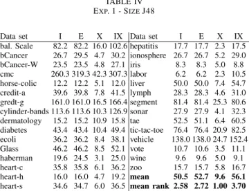
Looking at model sizes, in Table IV below, the results are as expected, i.e., more training instances results in larger J48 trees. Specifically, building the tree based on test instances only always resulted in the smallest tree. On average, the trees that are produced by X are less than one fifth of the size of the trees induced by I. So, if the purpose is to understand the random forest predictions, trees induced using X could provide very compact explanations.
TABLE IV EXP. 1 - SIZEJ48
Data set I E X IX Data set I E X IX
bal. Scale 82.2 82.2 16.0 102.6 hepatitis 17.7 17.7 2.3 17.5 bCancer 26.7 29.5 4.7 30.2 ionosphere 26.7 26.7 5.2 29.0 bCancer-W 23.5 23.5 4.8 27.1 iris 8.3 8.3 5.0 8.8 cmc 260.3 319.3 42.3 307.3 labor 6.2 6.2 2.3 10.5 horse-colic 12.2 12.2 5.1 12.0 liver 50.0 50.0 7.4 54.7 credit-a 39.6 39.8 7.8 41.5 lymph 28.3 28.3 4.6 31.0 gredt-g 161.0 161.0 16.5 166.4 segment 81.4 81.4 25.3 80.6 cylinder-bands 113.6 113.6 10.3 126.9 sonar 27.9 27.9 4.1 32.3 dermatology 15.2 15.2 10.9 15.8 tae 52.5 51.1 6.4 60.5 diabetes 43.4 43.4 10.4 49.4 tic-tac-toe 76.4 76.4 20.9 82.5 ecoli 36.2 36.2 8.4 38.1 vehicle 138.0 138.0 24.7 152.4 Glass 46.2 46.2 8.5 52.1 vote 10.7 10.6 3.5 11.1 haberman 19.6 24.5 3.1 25.0 wine 9.6 9.6 5.0 9.1 heart-c 35.8 35.8 6.1 36.2 zoo 15.7 15.7 5.8 16.7 heart-h 16.0 16.0 4.7 19.2 mean 50.5 52.7 9.6 56.1 heart-s 34.6 34.7 6.0 36.5 mean rank 2.58 2.72 1.00 3.70
Looking at the mean ranks, X produced significantly smaller trees than all other setups, while I and E trees were signifi-cantly smaller than IX trees. Comparing absolute numbers, however, the difference in comprehensibility between I, E and IX, is actually marginal, on most data sets. In addition, it is fair to say that for a number of data sets (e.g. cmc, credit-g, cylinder-bands and vehicle) the trees built using I, E or IX are probably too complex to be deemed comprehensible. Still, a large majority of all J48 models built must be considered compact enough to allow human understanding and analysis.
Experiment 1 is summarized in Table V below, where a + (-) for a pair of methods indicates a statistically significant difference in favor of the row (column) method.
TABLE V
EXP. 1 - SIGNIFICANT DIFFERENCESJ48 Accuracy AUC Test Fid. Train Fid. Size Data set E X IX E X IX E X IX E X IX E X IX
I - - - - + - +
E - - - - + - +
X - - - + +
IX + + + + + + + -
-Turning to experiment 2, Table VI below, shows the accu-racy and AUC results for G-REX.
TABLE VI
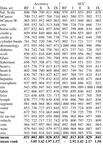
EXP. 2 - PREDICTIVE PERFORMANCE FORG-REX
Accuracy AUC Data set RF I E X IX RF I E X IX bal. Scale .806 .788 .790 .811 .806 .970 .853 .853 .893 .876 bCancer .700 .712 .697 .704 .716 .663 .580 .573 .592 .572 bCancer-W .965 .953 .952 .965 .963 .991 .951 .948 .963 .965 cmc .505 .552 .542 .513 .548 .708 .728 .719 .666 .731 horse-colic .857 .832 .841 .857 .856 .907 .799 .806 .834 .845 credit-a .859 .850 .849 .860 .863 .923 .856 .855 .865 .877 credit-g .758 .702 .698 .748 .738 .774 .671 .662 .640 .708 cylinder-bands .761 .702 .720 .746 .747 .902 .711 .721 .717 .738 dermatology .971 .955 .954 .947 .971 1.000 .988 .988 .996 .996 diabetes .761 .742 .744 .758 .761 .823 .737 .743 .720 .767 ecoli .850 .821 .816 .849 .849 .987 .959 .956 .962 .968 Glass .791 .692 .693 .791 .790 .939 .814 .803 .870 .892 haberman .656 .707 .708 .671 .702 .636 .549 .551 .553 .551 heart-c .815 .776 .774 .813 .815 .895 .761 .750 .810 .813 heart-h .802 .768 .780 .805 .804 .883 .749 .761 .776 .803 heart-s .830 .787 .783 .827 .827 .897 .769 .757 .822 .815 hepatitis .832 .781 .778 .832 .832 .854 .609 .630 .673 .664 ionosphere .937 .905 .904 .937 .939 .983 .888 .886 .922 .922 iris .943 .950 .947 .943 .945 1.000 .994 .989 1.000 1.000 labor .872 .866 .857 .872 .876 .970 .850 .846 .842 .850 liver .723 .656 .658 .721 .717 .765 .641 .637 .705 .705 lymph .830 .777 .770 .830 .830 .938 .806 .760 .843 .836 segment .981 .968 .968 .963 .980 1.000 .994 .993 .997 .997 sonar .853 .736 .727 .853 .845 .937 .735 .724 .850 .847 tae .672 .581 .574 .662 .660 .849 .738 .725 .759 .773 tic-tac-toe .971 .954 .955 .959 .980 .998 .965 .964 .957 .986 vehicle .752 .722 .717 .732 .742 .870 .800 .797 .723 .809 vote .964 .957 .957 .963 .964 .992 .948 .947 .961 .964 wine .979 .941 .942 .979 .977 1.000 .968 .964 .987 .987 zoo .943 .940 .934 .943 .946 1.000 .988 .985 .976 .980 mean .831 .802 .801 .828 .833 .902 .813 .810 .829 .841 mean rank - 3.05 3.42 1.97 1.57 - 2.92 3.42 2.17 1.50
The first impression is probably that the results are very similar to the first experiment. There is, however, one major difference; the results obtained by X are here more like IX than I and E. The explanation is that G-REX actually optimizes accuracy (here fidelity), while J48 optimizes the information gain. IX is, however, still more accurate and has higher AUC than X. Overall, X and IX are significantly more accurate than I and E, so the oracle coaching pays off also when evolving the decision tree. Again, IX mean test accuracy is actually higher than the accuracy obtained by the random forest. IX AUC is again significantly higher than I and E, while X has significantly higher AUC than I. A quick comparison between J48 and G-REX results (this is analyzed in more detail later in the paper) shows that the predictive performance is comparable, with the exception of the X setup, where G-REX is clearly better.
Looking at the G-REX fidelities in Table VII below, the most striking result is that X now obtains over 98% test fidelity, which is even higher than IX. This coupled with the quite low training fidelitys, clearly show that X by focusing solely on high test fidelity, produces very specialized models. All in all, X obtained significantly higher test fidelity than all other setups, while IX, at the same time, had significantly higher test fidelity than I and E. Comparing training fidelities, E has the highest overall mean, even if the results for I of course are identical on many data sets. The only statistically
significant differences are, however, that all other setups have higher training fidelity than X. So, even if the differences often are small, the effects of G-REX targeting fidelity more directly, are obvious in the results.
TABLE VII
EXP. 2 - FIDELITIES FORG-REX
Test fidelity Train fidelity
Data set I E X IX I E X IX bal. Scale .871 .875 .961 .958 .905 .905 .705 .902 bCancer .808 .781 .984 .937 .881 .889 .689 .882 bCancer-W .969 .967 1.000 .991 .980 .980 .935 .979 cmc .646 .643 .868 .728 .650 .655 .507 .646 horse-colic .922 .923 .998 .991 .934 .933 .821 .920 credit-a .915 .914 .982 .976 .929 .932 .838 .928 credit-g .803 .798 .960 .911 .830 .829 .691 .825 cylinder-bands .708 .718 .973 .861 .845 .848 .592 .831 dermatology .954 .954 .973 .978 .979 .978 .794 .974 diabetes .866 .866 .972 .966 .883 .881 .725 .881 ecoli .899 .892 .991 .985 .929 .928 .747 .933 Glass .769 .775 .998 .979 .944 .944 .526 .949 haberman .778 .787 .970 .891 .847 .845 .692 .843 heart-c .854 .854 .996 .975 .929 .934 .727 .917 heart-h .879 .870 .991 .976 .917 .915 .781 .914 heart-s .883 .871 .998 .979 .917 .924 .742 .914 hepatitis .848 .840 1.000 .992 .971 .972 .791 .969 ionosphere .933 .932 .999 .986 .970 .969 .795 .963 iris .976 .975 1.000 .997 .983 .984 .883 .983 labor .882 .860 1.000 .992 .991 .992 .734 .989 liver .761 .768 .985 .963 .902 .902 .614 .897 lymph .837 .810 1.000 .973 .944 .953 .691 .954 segment .974 .972 .979 .996 .991 .992 .902 .992 sonar .781 .774 1.000 .984 .959 .956 .632 .962 tae .747 .758 .986 .952 .852 .872 .434 .870 tic-tac-toe .945 .946 .986 .981 .989 .989 .702 .990 vehicle .796 .791 .939 .913 .868 .869 .614 .864 vote .977 .977 1.000 .997 .984 .983 .947 .981 wine .952 .951 1.000 .998 .990 .991 .796 .989 zoo .933 .934 1.000 .990 .995 .993 .765 .995 mean .862 .859 .983 .960 .923 .925 .727 .921 mean rank 3.38 3.62 1.07 1.93 1.85 1.68 4.00 2.47
Model sizes for G-REX follow the same pattern as for J48, i.e., X models are significantly more compact than all other setups, see Table VIII below.
TABLE VIII EXP. 2 - SIZEG-REX
Data set I E X IX Data set I E X IX bal. Scale 94.0 95.0 31.5 96.7 hepatitis 34.7 35.7 4.0 36.9 bCancer 67.4 71.4 11.6 73.0 ionosphere 24.2 24.2 9.0 20.0 bCancer-W 23.4 22.9 6.2 22.0 iris 9.8 10.4 5.2 9.6 cmc 98.0 97.4 71.1 97.9 labor 11.5 11.9 3.1 12.3 horse-colic 44.5 44.6 7.0 36.5 liver 84.6 84.4 16.1 85.3 credit-a 62.3 65.8 12.2 63.4 lymph 36.0 40.2 6.0 42.8 gredt-g 97.9 97.8 26.1 97.8 segment 88.6 89.0 27.1 91.4 cylinder-bands 77.0 79.3 20.7 74.9 sonar 40.7 40.9 8.2 46.2 dermatology 17.2 17.2 15.4 17.2 tae 60.5 63.6 13.6 67.4 diabetes 88.0 85.2 17.9 87.4 tic-tac-toe 95.1 95.4 46.6 94.3 ecoli 46.0 45.4 13.1 50.4 vehicle 98.8 98.9 33.4 99.0 Glass 64.7 64.0 17.1 63.9 vote 19.1 19.1 5.5 16.1 haberman 41.5 39.0 13.3 42.2 wine 10.1 10.5 6.3 9.3 heart-c 58.7 60.4 10.6 52.3 zoo 21.0 20.7 9.6 21.7 heart-h 47.2 45.8 8.5 47.0 mean 53.4 54.0 16.2 53.8 heart-s 40.6 44.9 9.9 39.6 mean rank 2.92 3.03 1.00 3.05
Overall, G-REX models are actually slightly larger than corresponding J48 models, especially for the X setup. Table IX below summarizes the results from experiment 2.
TABLE IX
EXP. 2 - SIGNIFICANT DIFFERENCESG-REX
Accuracy AUC Test Fid. Train Fid. Size Data set E X IX E X IX E X IX E X IX E X IX
I - - - +
-E - - - +
-X + + + - - + +
IX + + + + - +
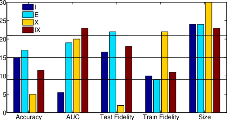
-Figure 2 below shows pair-wise comparisons between J48 and G-REX, for all setups. Bars show the number of data sets where J48 outperform G-REX, with regard to that specific metric. With 30 data sets, a standard sign test requires 21 wins, so bars higher than 21 indicate a significant difference in favor of J48, while bars lower than9 are significant in favor of G-REX.
Accuracy AUC Test Fidelity Train Fidelity Size 0 5 10 15 20 25 30 I E X IX
Fig. 2. Pair-wise comparisons. Bars show the number of wins for J48 against the corresponding G-REX setup
There are a number of interesting observations in this chart. First of all, it is obvious that oracle coached G-REX models clearly outperform their J48 counterparts, with regard to accuracy. Looking specifically at the X setup, G-REX models are significantly more accurate, due to a significantly higher test fidelity. J48, on the other hand, obtain generally higher AUCs (with the exception of standard rule induction I), and produces significantly more compact models, for all setups. Summarizing this comparison, G-REX would be the choice of technique for the oracle coaching (X and IX), if accuracy is prioritized and the slightly larger models are acceptable. For the most basic task (inducing or evolving trees directly from the data set) the techniques win 15 data sets each, with regard to accuracy. G-REX trees have, however, significantly higher AUCs, but are also significantly larger. When used as rule extractors (E) finally, there are only small differences in accuracy and AUC, but the the small advantage for J48 is due to higher test fidelity, which probably is the result of smaller trees, generalizing better to the unseen data; i.e., the larger G-REX trees have overfit the training data slightly.
In order to understand how the oracle coached single tree models are able to obtain accuracies comparable to the random forest, without producing gigantic trees with perfect fidelities, a deepened analysis is necessary. For this analysis we define the following measures:
• Correct fidelityis the proportion of production instances correctly predicted by the oracle that was also correctly predicted by the coached model.
• Incorrect fidelity is the proportion of production in-stances that was initially wrongly predicted by the oracle, and then also incorrectly predicted by the coached model. • Correct infidelity is the proportion of production in-stances that was initially wrongly predicted by the oracle, but then correctly predicted by the coached model. • Incorrect infidelity is the proportion of production
in-stances that was initially correctly predicted by the oracle, but then incorrectly predicted by the coached model. Table X below shows correct fidelities (CF) and correct infidelities (CI), as defined above, for the X and IX setups.
TABLE X FIDELITY ANALYSIS J48 G-REX X IX X IX Data set CF CI CF CI CF CI CF CI bal. Scale .950 .185 .992 .028 .988 .076 .989 .049 bCancer .940 .162 .954 .166 .991 .034 .967 .131 bCancer-W .989 .085 .995 .004 1.000 .004 .994 .093 cmc .868 .145 .924 .107 .859 .171 .819 .278 horse-colic .984 .046 .993 .055 .999 .006 .994 .027 credit-a .980 .125 .990 .063 .990 .067 .988 .099 gredit-g .959 .082 .972 .060 .967 .060 .928 .143 cylinder-bands .900 .069 .963 .181 .927 .005 .831 .036 dermatology .987 .103 .988 .318 .971 .533 .989 .716 diabetes .966 .087 .961 .102 .979 .052 .978 .071 ecoli .961 .051 .990 .063 .995 .024 .991 .046 glass .870 .038 .984 .011 .999 .004 .986 .047 haberman .907 .327 .957 .231 .989 .065 .952 .226 heart-c .963 .089 .991 .068 .997 .005 .985 .068 heart-h .963 .141 .969 .101 .997 .029 .986 .065 heart-s .967 .070 .990 .033 .997 .000 .986 .057 hepatitis .958 .103 .974 .057 1.000 .000 .995 .023 ionosphere .989 .050 .997 .032 .999 .000 .993 .122 iris .999 .047 .999 .000 1.000 .000 .999 .047 labor .942 .027 .978 .068 1.000 .000 .998 .041 liver .897 .141 .947 .088 .988 .023 .970 .055 lymph .942 .043 .980 .063 .994 .000 .978 .031 segment .984 .061 .997 .063 .981 .084 .997 .068 sonar .965 .049 .987 .013 1.000 .000 .986 .029 tae .792 .085 .975 .052 .983 .004 .957 .052 tic-tac-toe .905 .069 .989 .536 .987 .033 .995 .478 vehicle .952 .059 .967 .093 .955 .057 .944 .131 vote .988 .101 .999 .076 1.000 .000 .999 .057 wine .996 .000 .998 .000 1.000 .000 .998 .000 zoo .815 .000 .998 .207 1.000 .000 .998 .086 mean .943 .088 .980 .098 .984 .045 .972 .112
The correct fidelity scores show that the vast majority of all instances correctly classified by the random forest are also correctly classified by the coached model. When averaging over all data sets, all setups except J48(X) have a correct fidelity rate of over 97%. An even more interesting, and somewhat surprising, result is that as many as 10% of the
instances where the random forrest is wrong, are still predicted correctly by both J48 setups and G-REX(IX). As a matter of fact, the correct infidelities of both IX setups often more than compensates for the incorrect fidelities, producing single tree models that actually have higher accuracies than the random forest. So, the overall conclusion is that oracle coaching is able to mimic the performance of the random forest, not by explicitly copy its every prediction, but by using the oracle for building a fairly compact yet very accurate model.
V. CONCLUSION
We have in this paper shown that it is often possible to approximate a random forest, with good precision, using just one decision tree. From the results, it is obvious that the oracle coaching produced very accurate models, clearly comparable to the the random forest, on the specific test data. Models evolved using only oracle data were very compact and ex-tremely accurate, thus providing comprehensible explanations of the predictions. The best results overall were, however, obtained by combining training and oracle data, resulting in models significantly more accurate than models induced or evolved directly from the data. As demonstrated, most extracted models were not overly complex, indicating that the oracle data was not severely overfit. This was also verified when the analysis found the number of correct infidelities to be considerable, on many data sets. Comparing J48 and G-REX, most differences were, in absolute numbers, fairly small. Still, in the oracle coaching setting, G-REX produced significantly more accurate models, compared to J48. Regarding model sizes, J48 models were, on the other hand, generally more compact than the corresponding G-REX models. More impor-tantly, though, almost all models were compact enough to be considered comprehensible. Based on this, we conclude that oracle coaching is a powerful tool for providing explanations of ensemble predictions, and for enabling human analysis of complex ensemble models.
ACKNOWLEDGMENT
This work was supported by the INFUSIS project www. his.se/infusis at the University of Skövde, Sweden, in part-nership with the Swedish Knowledge Foundation under grant 2008/0502.
REFERENCES
[1] T. G. Dietterich, “Machine-learning research: Four current directions,”
The AI Magazine, vol. 18, no. 4, pp. 97–136, 1998.
[2] L. Breiman, “Random forests,” Machine Learning, vol. 45, no. 1, pp. 5–32, October 2001.
[3] P. Goodwin, “Integrating management judgment and statistical methods to improve short-term forecasts,” Omega, vol. 30, no. 2, pp. 127 – 135, 2002.
[4] J. R. Quinlan, C4.5: programs for machine learning. Morgan Kaufmann Publishers Inc., 1993.
[5] L. Breiman, J. Friedman, C. J. Stone, and R. A. Olshen, Classification
and Regression Trees. Chapman & Hall/CRC, January 1984. [6] R. Andrews, J. Diederich, and A. B. Tickle, “Survey and critique of
techniques for extracting rules from trained artificial neural networks,”
Knowl.-Based Syst., vol. 8, no. 6, pp. 373–389, 1995.
[7] M. W. Craven and J. W. Shavlik, “Extracting tree-structured repre-sentations of trained networks,” in Advances in Neural Information
Processing Systems. MIT Press, 1996, pp. 24–30.
[8] U. Johansson, C. Sönströd, and T. Löfström, “Oracle coached decision trees and lists,” in IDA, ser. Lecture Notes in Computer Science, P. R. Cohen, N. M. Adams, and M. R. Berthold, Eds., vol. 6065. Springer, 2010, pp. 67–78.
[9] S. K. Murthy, “Automatic construction of decision trees from data: A multi-disciplinary survey,” Data Mining and Knowledge Discovery, vol. 2, pp. 345–389, 1998.
[10] A. Tsakonas, “A comparison of classification accuracy of four genetic programming-evolved intelligent structures,” Information Sciences, vol. 176, no. 6, pp. 691 – 724, 2006.
[11] C. Bojarczuk, H. Lopes, and A. Freitas, “An innovative application of a constrained-syntax genetic programming system to the problem of predicting survival of patients,” in Genetic Programming, ser. Lecture Notes in Computer Science, C. Ryan, T. Soule, M. Keijzer, E. Tsang, R. Poli, and E. Costa, Eds. Springer Berlin / Heidelberg, 2003, vol. 2610, pp. 11–59.
[12] M. W. Craven and J. W. Shavlik, “Using neural networks for data mining,” Future Gener. Comput. Syst., vol. 13, no. 2-3, pp. 211–229, 1997.
[13] S. Thrun, G. Tesauro, D. Touretzky, and T. Leen, “Extracting rules from artificial neural networks with distributed representations,” in Advances
in Neural Information Processing Systems 7. MIT Press, 1995, pp. 505–512.
[14] O. Chapelle, B. Schölkopf, and A. Zien, Eds., Semi-Supervised Learning. Cambridge, MA: MIT Press, 2006.
[15] T. Joachims, “Transductive inference for text classification using support vector machines.” Morgan Kaufmann, 1999, pp. 200–209.
[16] B. Settles, “Active learning literature survey,” University of Wisconsin – Madison, Computer Sciences Technical Report 1648, 2009. [17] U. Johansson, R. König, and L. Niklasson, “Rule extraction from trained
neural networks using genetic programming,” in ICANN, supplementary
proceedings, 2003, pp. 13–16.
[18] U. Johansson, Obtaining Accurate and Comprehensible Data Mining
Models: An Evolutionary Approach. PhD-thesis. Institute of Technol-ogy, Linköping University, 2007.
[19] R. König, U. Johansson, and L. Niklasson, “G-REX: A versatile framework for evolutionary data mining.” in ICDM Workshops. IEEE Computer Society, 2008, pp. 971–974.
[20] U. Johansson and L. Niklasson, “Evolving decision trees using oracle guides,” in CIDM. IEEE, 2009, pp. 238–244.
[21] I. H. Witten and E. Frank, Data Mining: Practical Machine Learning
Tools and Techniques, Second Edition (Morgan Kaufmann Series in Data Management Systems). Morgan Kaufmann, June 2005.
[22] R. König, U. Johansson, T. Löfström, and L. Niklasson, “Improving gp classification performance by injection of decision trees,” in IEEE
Congress on Evolutionary Computation. IEEE, 2010, pp. 1–8. [23] A. Frank and A. Asuncion, “UCI machine learning repository,” 2010.
[Online]. Available: http://archive.ics.uci.edu/ml
[24] J. Demšar, “Statistical comparisons of classifiers over multiple data sets,”
J. Mach. Learn. Res., vol. 7, pp. 1–30, 2006.
[25] M. Friedman, “The use of ranks to avoid the assumption of normality implicit in the analysis of variance,” Journal of American Statistical
Association, vol. 32, pp. 675–701, 1937.
[26] P. B. Nemenyi, Distribution-free multiple comparisons. PhD-thesis. Princeton University, 1963.