2016:05 Technical Note, Assessment of SKB TR-14-15 Assessment of SKB TR-14-15 “Possible influence from stray currents from high voltage DC power transmission on copper canisters”

Technical Note

Assessment of SKB TR-14-15 “Possible influence

from stray currents from high voltage DC power

transmission on copper canisters”

2016:05

SSM perspektiv

Bakgrund

Strålsäkerhetsmyndigheten (SSM) granskar Svensk Kärnbränslehantering AB:s

(SKB) ansökningar enligt lagen (1984:3) om kärnteknisk verksamhet om upp­

förande, innehav och drift av ett slutförvar för använt kärnbränsle och av en

inkapslingsanläggning. Som en del i granskningen ger SSM konsulter uppdrag

för att inhämta information i avgränsade frågor. I SSM:s Technical note­serie

rapporteras resultaten från dessa konsultuppdrag.

Syfte

Det övergripande syftet med denna rapport är att ta fram synpunkter på SKB:s

säkerhetsredovisning SR­Site eller dess underlagsrapporter. Specifikt för denna

rapport är syftet att granska SKB:s redovisning av eventuell påverkan på slutför­

varet av läckströmmar från högspänningskablar.

Författarens sammanfattning

I denna rapport sammanfattas först bakgrundsmaterial som ingår i en simulerings­

modell för beräkning av vertikala elektriska spänningsfall över deponeringshål. De

viktigaste parametrarna för bestämning av detta spänningsfall är den elektriska

ledningsförmågan (eller den inversa storleken resistiviteten) av ben tonit leran som

används som fyllnadsmaterial i det förseglade slutförvaret, strömstyrkan i elektro­

den och avståndet från slutförvaret till elektroden. Däremot har den elektriska

ledningsförmågan hos bergarterna i Forsmarksområdet ganska liten betydelse för

bestämningen av ”batteri”­spänningen i slutförvaret.

Bentonitleran som fyller deponeringshålen och det mesta av de förseglade

delarna av slutförvaret antas vara vattenmättad och allt vatten antas stanna kvar

i deponeringshålen. Detta är mycket viktigt för att upprätthålla ett lågt elektriskt

motstånd i deponeringshålet och ett lågt spänningsfall över kopparkapseln.

Geometrin i FEM­modellen innehåller en förenklad beskrivning av depone­

ringstunnlar, schakt och transporttunnlar, men inte detaljerna i själva depo­

neringshålen. FEM­simuleringar visar att en ekvivalent elektrisk krets med

en batterispänning och ett inre motstånd är tillräcklig för att beräkna det

vertikala spänningsfallet under deponeringstunnlarna för ett givet elektriskt

motstånd av deponeringshålet.

Fyra olika simulerade scenarier har beskrivits. Två av dessa relaterar till de nuva­

rande förhållandena kring Forsmark och de verkar beskriva spänningsförhållan­

dena i slutförvaret realistiskt om Skan­Link transmitterar energi i enbart en kabel.

De övriga två scenarierna beskriver fall utgående från den hypotetiska händelsen

att en elektrod någon gång i framtiden kommer att placeras rakt över eller nära

slutförvaret.

Den maximala spänningen över en given kopparkapsel beräknas att vara mindre

än 500 mV, vilket indikerar att korrosionsströmmar ligger i det linjära område där

kopparkapseln kan karakteriseras ha ett högt korrosionsmotstånd så att de möj­

liga korrosionsströmmarna blir mycket låga.

SSM 2016:05

Effekten av ”Geomagnetically Induced Currents” (GIC) kan ge upphov till spän­

ningar över kopparkapslar större än 500 mV, men bara i korta tidsintervall av

storleksordning en timma vid kraftiga geomagnetiska stormar. Ju längre avstån­

det är mellan jordningspunkter i ett högspänningsnät desto större är spänningen

mellan dem och desto större blir strömmen i jordningspunkten.

En viss osäkerhet finns gällande själva FEM­programmet som har använts. Det

testades mot en enkel kil­modell, för vilken en analytisk lösning finns, där all

ström är riktad radiellt bort från elektroden så att ingen ström flyter vinkelrätt

mot gräns ytor där ledningsförmågan ändras diskontinuerligt. Resultaten av denna

simulering visade mycket bra överensstämmelse med den analytiska lösningen.

Emellertid blev en mera komplicerad modell inte validerat mot oberoende simu­

leringar, antingen analytiska lösningar (en referens till en sådan lösning har

angetts) eller modell beräkningar med till exempel integralekvationsmetoden.

Speciellt lämpar sig scenario 1 med bara en deponeringstunnel bra åt en lösning

med den senare metoden. Ytterligare tester med bra överensstämmelse skulle öka

tillförlitligheten av de beräknade batterispänningarna.

Projekt information

Kontaktperson på SSM: Lena Sonnerfelt

Diarienummer ärende: SSM2015­3998

Aktivitetsnummer: 3030012­4118

SSM perspective

Background

The Swedish Radiation Safety Authority (SSM) reviews the Swedish

Nuclear Fuel Company’s (SKB) applications under the Act on Nuclear

Activities (SFS 1984:3) for the construction and operation of a reposi­

tory for spent nuclear fuel and for an encapsulation facility. As part of

the review, SSM commissions consultants to carry out work in order to

obtain information on specific issues. The results from the consultants’

tasks are reported in SSM’s Technical Note series.

Objective

The general objective of the present project is to provide independ­

ent review comments for one area of SKB:s post closure safety analysis,

SR­Site. With this in mind, the purpose of this report is to review SKB’s

presentation on possible influence from stray currents from high voltage

DC power transmission on a repository for nuclear fuel.

Summary by the author

In this report background material for setting up a simulation model for

calculating the vertical electrical voltage drops over deposition holes is

first summarized. The main factor controlling this voltage is the elec­

trical resistivity of the bentonite clay filling the sealed repository, the

amount of current injected at an electrode and the distance from the

repository to the electrode. The electrical resistivity of the background

medium below the Forsmark repository level has small influence on the

“battery” voltage at the repository.

The bentonite clay filling most of the sealed parts of the repository

and the deposition holes is water saturated and no water is assumed to

escape from the deposition holes with time. This is very important for

keeping a low resistance of a deposition hole and hence a low battery

voltage over the copper canister.

The geometry of the FEM model contains representations of the deposi­

tion tunnels, shafts and ramp, but not of the details of the deposition

holes. The FEM simulations prove that an equivalent electrical circuit

with a battery voltage and an internal resistance is sufficient for calcu­

lating the vertical voltage drop below the deposition tunnels once the

total resistance of the deposition system is fixed.

Then the four different scenarios simulated are discussed. Two scenarios

relate to the present situation at Forsmark and it is believed that they

realistically describe the voltage conditions at repository level when the

Skan­Link transmits energy in only one cable. Two scenarios relate to a

rather improbable situation where an electrode is located right on top

of or close by the repository.

The four scenarios studied all had maximum battery voltages below

500 mV which indicates that corrosion currents lie in the linear range

where the copper canister can be characterized by a high corrosion

SSM 2016:05

The effect of Geomagnetically Induced Currents can give rise to voltages

over copper canisters greater than 500 mV, but only for a very short time

interval. The longer the distance is between grounding points in a power

network the greater is the voltage between them and the greater is the

grounding current.

A main concern is the FEM code itself. The code was tested for a simple

wedge model where all currents flow radially whereby no charges are

produced when currents cross resistivity interfaces. This simulation was

in very good agreement with the analytical solution. However, a more

complicated model was not tested against independent simulations,

either analytical solutions (a reference to one such solution is given) or

simulations using for example integral equations. Especially a simplified

scenario 1 with only one deposition tunnel would be easy to check with

the latter method.

If such tests show a reasonable agreement it would strongly enhance

the credibility of the calculated battery voltages.

Project information

2016:05

Author: Laust B Pedersen

Uppsala University, Uppsala, Sweden

Assessment of SKB TR-14-15 “Possible influence

from stray currents from high voltage DC power

transmission on copper canisters”

SSM 2016:05

This report was commissioned by the Swedish Radiation Safety Authority

(SSM). The conclusions and viewpoints presented in the report are those

of the author(s) and do not necessarily coincide with those of SSM.

Summary:

In this report background material for setting up a simulation model for calculating the vertical electrical voltage drops over deposition holes is first summarized. The main factor controlling this voltage is the electrical resistivity of the bentonite clay filling the sealed repository, the amount of current injected at an electrode and the distance from the repository to the electrode. The electrical resistivity of the background medium below the Forsmark repository level has small influence on the “battery” voltage at the repository.

The bentonite clay filling most of the sealed parts of the repository and the deposition holes is water saturated and no water is assumed to escape from the deposition holes with time. This is very important for keeping a low resistance of a deposition hole and hence a low battery voltage over the copper canister.

The geometry of the FEM model contains representations of the deposition tunnels, shafts and ramp, but not of the details of the deposition holes. The FEM simulations prove that an equivalent electrical circuit with a battery voltage and an internal resistance is sufficient for calculating the vertical voltage drop below the deposition tunnels once the total resistance of the deposition system is fixed.

Then the four different scenarios simulated are discussed. Two scenarios relate to the present situation at Forsmark and it is believed that they realistically describe the voltage conditions at repository level when the Skan-Link transmits energy in only one cable. Two scenarios relate to a rather improbable situation where an electrode is located right on top of or close by the repository.

The four scenarios studied all had maximum battery voltages below 500 mV which indicates that corrosion currents lie in the linear range where the copper canister can be characterized by a high corrosion resistance so that possible corrosion currents are very small.

The effect of Geomagnetically Induced Currents can give rise to voltages over copper canisters greater than 500 mV, but only for a very short time interval. The longer the distance is between grounding points in a power network the greater is the voltage between them and the greater is the grounding current.

A main concern is the FEM code itself. The code was tested for a simple wedge model where all currents flow radially whereby no charges are produced when currents cross resistivity interfaces. This simulation was in very good agreement with the analytical solution. However, a more complicated model was not tested against independent simulations, either analytical solutions (a reference to one such solution is given) or simulations using for example integral equations. Especially a simplified scenario 1 with only one deposition tunnel would be easy to check with the latter method.

If such tests show a reasonable agreement it would strongly enhance the credibility of the calculated battery voltages.

Contents

Summary: ... 1

1. Introduction ... 5

2. Calculation of potential drops over deposition holes ... 7

2.1 SKB’s presentation ... 7

2.1.1. Voltage measurements ... 7

2.1.2 Influence of the sea ... 7

2.1.3 Influence of the earth’s upper crust ... 8

2.1.4 Model representation of the repository ... 8

2.1.5 Model representation of the HVDC electrode ... 8

2.1.6 Scenario 1. Uniform electric field resulting from a remote electrode with uniform deposition holes ... 8

2.1.7 Scenario 2. Forsmark Power station as a secondary electrode ... 8

2.1.8 Scenarios 3 and 4. Possible future HVDC electrode at various distances from the repository ... 9

2.1.9 The voltage along the copper canister in a deposition hole ... 9

2.1.10 The current through the copper canister in a deposition hole ... 10

2.2 Assessment of results ... 10

2.2.1 Background resistivity in the upper crust ... 10

2.2.2 Calculated and measured voltages at the surface ... 11

2.2.3 The FEM code ... 11

2.2.4 Scenario 1 ... 11

2.2.5 Scenario 2 ... 11

2.2.6 Scenarios 3 and 4 ... 12

2.2.7 The voltage along the copper canister in a deposition hole and the current through the copper canister ... 12

3. The four scenarios ... 13

3.1. SKB’s presentation ... 13

3.1.1. Land uplift and sea level changes ... 13

3.2. Assessment ... 13

4. Telluric currents ... 15

4.1. Calculation of maximum electrical field without grounding points ... 15

4.2. The Consultants’ assessment ... 17

1. Introduction

High Voltage Direct Current (HVDC) technology is used to transmit electric power over long distances such as is the case between Sweden and Finland in the so-called Fenno-Skan cable. The cable is grounded in Sweden at Fågelsundet, located about 25 km north of the Forsmark nuclear power station with the other grounding point located about 200 km away close to the Finnish coast.

HVDC power transmission can take place using either one or two cables. If only one cable is in use the return current is transmitted through the earth/sea system, and with two cables it is possible to balance the two currents so that virtually no DC current is injected into the earth/sea. In the former case stray currents spread out from the grounding point and at small distances away from a grounding point compared with the distance between the two grounding points the current system can be well approximated by considering only the closest grounding point. Thus to calculate the currents inside the earth up to distances of 25 km from the grounding point at Fågelsundet it is only necessary to consider the current injected at Fågelsundet and disregard the oppositely directly current in Finland.

DC stray currents decay slowly with distance away from grounding points and therefore large electric fields can be observed at several km away from grounding points carrying a few thousand A. Directly below a grounding point the electric field is entirely vertical and at large distances the field is dominantly horizontal even at 500 m depth. At current densities some distance away the electrodes at the grounding point Ohm’s law is valid, stating that the current density, j [A/m2_{] is} directly proportional to the prevailing electric field, E [V/m]

𝒋 = 𝜎𝑬 =1

𝜌𝑬,

where 𝜎 and 𝜌 are the electrical conductivity [S/m] and resistivity [Ohm-m], respectively. Thus, for high electrical resistivity the current density will be small and vice versa. By integrating the current density over a given area the total current, I passing through that area can then easily be calculated. In the end the amount of current in a copper canister is an important factor for controlling the amount of corrosion.

In this report the details relating to corrosion will not be reviewed. Only the aspects related to the estimates of possible electric fields (voltage gradients) over copper canisters in deposition holes in a nuclear waste repository of the Forsmark type will be considered.

TR-14-15 presents detailed calculations of the vertical electric field from a variety of scenarios relating to geometry and distribution of electrical resistivity in the earth and in the repository. The first assumption made is that power transmission is monopolar (only one cable) even though nowadays the Fenno-Skan power transmission is bipolar most of time.

Four main scenarios are presented

1. A hypothetical case with a large horizontal field of 50 V/km impressed on the boundaries of a model of the repository.

SSM 2016:05 ₆

2. A realistic case describing the effect of the grounding of overhead lines close to the Forsmark power station leading to secondary currents into the ground of 20 A.

3. A hypothetical case with a future HVDC sea-based electrode operating at 2500 A located right above the repository.

4. A hypothetical case with a future HVDC sea-based electrode operating at 2500 A located at various distances from the repository.

In the following I will discuss each case separately with regard to the issues defined by SSM

 Are the potential drops over the deposition holes as shown in TR-14-15 correct?

 Are the four scenarios representative for the present and possible future location of grounding points for HVDC transmission and repository for nuclear waste?

 Influence of telluric currents on the potential drops over the deposition holes.

Appendix A include the results of calculations using simplified models to get an idea of the order of magnitude of the voltage drops found in TR-14-15. An annotated copy of TR-14-15 with comments is also included.

2. Calculation of potential drops over

deposition holes

The calculation of potential drops over a deposition hole is split up into several steps. In the first step the potential distribution is calculated using a FEM code without taking into account the details of the conditions in the deposition hole (spent nuclear fuel, copper canister, bentonite clay). The details of the FEM program or the description of the discretization used for the various cases are not presented. These calculations form the basis for setting up an equivalent electrical model in which the whole repository is represented by a battery with a given voltage (referred to as electro-motive force) and internal resistance. In the second step the electrical properties of the deposition hole are described by a combination of resistors representing the bentonite clay and the copper canister represented as a kind of diode with its polarization voltage and polarization resistance.

2.1 SKB’s presentation

2.1.1. Voltage measurements

The present situation with the electrode at Fågelsundet is described. Voltage measurements around Fågelsundet are shown as a function of distance away from the electrode. It is noticed that the voltage on the land side is much higher than the corresponding one on the sea side. The highest voltage registered at the shoreline, located 2.3 km away from the electrode, was 0.2 V/m and the voltage drop from 2.3 to 5 km away from the electrode was 200 V.

Voltage measurements around Forsmark show circular symmetry indicating that superimposed on the primary voltage distribution from current injected at Fågelsundet (calculated to 0.5 V/km) is a voltage generated by a point current injected close to Forsmark, increasing the gradient locally to 1.5 V/km. The point current is generated by local grounding lines that act as a short circuit to locally change the potential at a grounding point close to Forsmark. The resulting voltage distribution can be modelled approximately by a point electrode carrying 20 A.

2.1.2 Influence of the sea

The Fågelsundet electrode is located 2.3 km from the shoreline. Depending on the bathymetry of the sea a proportionally large part of the total current injected will be confined to the sea. Using a simple wedge model for the sea bottom with a slope of 0.001 and locating the electrode right on the shore predicts that the potential is reduced by a factor of about 3. The FEM model results agree very well with analytic solution for this simple case where all currents flow radially away from the electrode and they do not cross discontinuities in electrical resistivity.

SSM 2016:05 ₈

2.1.3 Influence of the earth’s upper crust

A number of stratified models for the Earth’s resistivity as a function of depth are used to model the potential distribution. The simplest one has a constant resistivity of 10000 Ohm-m and five other distributions have resistivities that decrease to about 1000 Ohm-m down to about 2000 m depth.

2.1.4 Model representation of the repository

Several different representations are used. For the scenarios 1 and 2 where currents are predominantly horizontal the repository model only contains horizontal deposition and main tunnels. For the scenarios 3 and 4 where vertical currents are significant the vertical shafts and ramp that connect the ground level to the repository level are included as well.

2.1.5 Model representation of the HVDC electrode

A detailed description of the HVDC electrode is used when the repository is located close to the electrode, namely scenarios 3 and 4. When located far away compared with the depth of the repository the electric field is taken to be horizontal and uniform and for scenario 2 when representing the secondary source in the Forsmark area a single point electrode is used.

2.1.6 Scenario 1. Uniform electric field resulting from a remote

electrode with uniform deposition holes

This case study is a realistic simulation of the conditions that would exist at the Forsmark repository if only one of the SCAN LINK cables were used for power transmission and a horizontal field of 50 V/km were produced at the repository. In the first simulations the deposition holes were assumed to have the same

electrical resistivity as the surrounding rock, i.e. close to 10000 Ohm-m. The voltage drops from 500 m to 508 m depth was calculated for various positions along the deposition tunnels. The largest voltage drop occurs close to the end of the tunnel where it reaches values in the range 2-5 V, which drops slowly to zero in the middle of the tunnel.

The next simulations describe how the voltage drop and the current in the deposition hole changes when its electrical resistivity is varied from 10000 m to 2 Ohm-m. The result shows that there is a linear relationship between voltage and current such that for large currents the voltage over the hole is small and vice versa. The slope of the relationship is effectively independent of the location of the deposition hole, leading to the idea to represent the tunnel system without the deposition holes as an equivalent electrical circuit with a “battery” of voltage from 2 – 5 V and an internal resistance of about 750 Ohm.

2.1.7 Scenario 2. Forsmark Power station as a secondary

electrode

Forsmark Power station is well grounded with a low resistance of about 5 Ohm. The potential drop from Forsmark to a remote site due to the HVDC current at

be 20 A. This is a much smaller current than the current impressed at Fågelsundet, but the distance from Forsmark to the center of repository system is only 800 m and therefore the effect on the vertical potential drop can be substantial.

Using a simplified model without the influence of the sea and without including vertical shafts and ramps the simulations give vertical voltage drops at deposition hole positions (but with the same high resistivity as the surrounding rock) of about 3 V. This is very close to the range calculated for scenario 1 and the internal resistance of the equivalent circuit is also close to 750 Ohm.

2.1.8 Scenarios 3 and 4. Possible future HVDC electrode at

various distances from the repository

Here is assumed that that the electrode is located 2 km from the shoreline and again that the slope of the seabed is 0.001. The model of the repository now include representations of the vertical shafts and ramps filled with bentonite clay from 200 m downwards and by crushed rock above that level. An effective layered model with varying conductivity as a function of depth is used to represent the combined effect of rocks, crushed rock, saline water in porous parts and bentonite clay above the deposition tunnels.

With a current of 2500 A impressed directly over the repository the maximum voltage drops were found close to the end of the deposition tunnels as before. But now the voltage drops were considerably higher, about 30 V.

Many examples were finally presented with varying distance between the electrode and depository. Not surprisingly the voltage drops were reduced with increasing distance.

2.1.9 The voltage along the copper canister in a deposition hole

The bentonite in the deposition holes is assumed to form a closed system with respect to water loss with time. A linear relation between water content and electrical conductivity is assumed and in that case it is shown that the total vertical conductance of the bentonite in the deposition hole is essentially independent of how the water is distributed away from the copper canister to the wall of the deposition hole. In Appendix A a general proof for that is given.

The total resistance of the bentonite in a deposition hole is calculated to vary from 7.4 Ohm to 2.3 Ohm corresponding to 17 and 28 % water, respectively. The so-called polarization resistance, i.e. the resistance to drive currents through the copper canister, is supposed to be independent on voltage and equal to 3580 Ohm for oxygen free conditions. This is much larger than the resistance of the bentonite part of the current path and the voltage across the canister is largely independent of the polarization resistance.

The voltage across the copper canister (that drives the current through it) is then entirely determined by the voltage across the deposition hole that would exist if the copper canister and the fuel inside were replaced with insulating material.

The voltage across the deposition holes can then be calculated from the equivalent circuit once the “battery” voltage, the internal resistance and the bentonite resistance in the deposition hole are specified. Once the equivalent circuit is specified the only difference between the four scenarios is the difference in the distribution of

SSM 2016:05 ₁₀

Typical maximum values for the calculated voltages along the copper canister close to the end walls of deposition tunnels are 100-200 mV, 30-60 mV, 200-300 mV, 200-300 mV for scenarios 1, 2, 3 and 4, respectively. For scenario 3 an extra simulation with the repository located at a depth of 700 m depth instead of 500 m give slightly lower values.

2.1.10 The current through the copper canister in a deposition

hole

A polarization resistance of 3580 Ohm was measured under oxygen free conditions which are the conditions expected to prevail in the repository except for the initial phase after deposition. This value of the polarization resistance was obtained experimentally with a potential difference of 365 mV around the so-called corrosion potential. Referring to other experimental data (King and tang, 1998) it is argued that the high polarization resistance prevails for voltages smaller than 500 mV. Referring to section 2.1.9 above we note that all maximum voltages lie below 500 mV limit and hence the high polarization resistance can be used to determine the current through the copper canister. With 500 mV across the canister a corrosion rate of 0.2 µm/year is estimated. The corresponding typical maximum corrosion rates for the four scenarios are smaller than that, typically 40-80 nm/year, 1.2-2.4 nm/year, 80-120 nm/year and 80-120 nm/year, respectively.

2.2 Assessment of results

2.2.1 Background resistivity in the upper crust

It can be argued that the chosen decreasing resistivity with depth in the upper crystalline crust is improbable since the amount of a conducting phase in crystalline rocks decrease because porosity generally decreases with increasing pressure (depth). Only if a conducting phase in the form of graphite or sulphides in the upper crust (typically the upper 20 km in this part of Sweden) is present can the resistivity decrease to much lower values. In Norrland such mineralizations are common, but not in the Uppland area.

Generally speaking, if the resistivity decreases with depth a larger proportion of the current will be found at depth compared with the case where the resistivity is independent of depth. This also means that the vertical gradient (the vertical electric field) at a given location close to the surface becomes slightly larger. The reason for choosing six different models for the resistivity distribution in the upper crust is that the authors believe that some models give better agreement with the measured data than others. This will be discussed later in the assessment. However, the many examples with different models of the crustal resistivity distribution are superfluous, and it would be sufficient to show in just one example that the calculated voltage drops are effectively independent of the chosen resistivity distributions. The report would be easier to read and considerably shorter as well.

2.2.2 Calculated and measured voltages at the surface

The lack of agreement between measured and calculated voltage from the electrode at Fågelsundet is explained partly as a result of using the wrong background resistivity depth variation. Probably this is not the main reason for the disagreement. Instead, by taking into account that the water depth variation is much more

complicated than the simple slope model used the agreement between measurements on land and model calculations becomes much better as shown in Appendix A.

2.2.3 The FEM code

It is difficult to assess the accuracy of the numerical calculations. One example is given to show the agreement between an analytic solution and a numerical solution. The voltage distribution from a simple wedge model representing the deepening sea over the earth’s crust away from the shoreline is shown in Figure 4-22 for both solutions. The agreement is excellent. However, the source is located right at the coast line so that all currents flow radially and no currents cross the interface between sea and crust.

When currents cross interfaces electrical surface charges are generated to account for the discontinuity of the electric field orthogonal to the interface. It is

recommended that such a test be carried out because in the simulations of the voltages at the repository such currents play a dominant role as sources for the vertical electric field in the deposition holes.

An analytic solution exists for the wedge model where the electrode is located in the sea away from the coast (Maeda, 1955; Hunt et al., 2001). A good agreement with this solution would ensure that the fundamental physics is taken into account. Another model that can easily be tested using an integral equation approach is the model used in scenario 1 where a homogeneous horizontal field is impressed.

2.2.4 Scenario 1

A primary horizontal electric field of 50 V/km represents a typical electric field at Forsmark generated by an electrode at FågelsundetThe calculated voltage drops over future deposition holes (length 8 m) close to the end faces of (not excavated yet) are typically 3-5 V, corresponding to an average vertical electric field below the floor of the deposition tunnels of 375-625 V/km.

Such large vertical electric fields were puzzling and the author made a simplified calculation of the same field assuming that only one tunnel was present using a so-called Born approximation (see Appendix A for more details). The calculated voltage drop 5 m away from the end face was only 0.02 V decaying very rapidly from the end face. The author would have liked to solve the problem without the Born approximation, but insufficient time was availableto set up the integral equation and solve it numerically.

Under all circumstances the large voltage drop reported in TR-14-15 intriguingly is high and it is recommended that an independent test calculation be carried out.

2.2.5 Scenario 2

SSM 2016:05 ₁₂

injected. A current of 20 A was chosen, which is believed to be a good estimate of a realistic maximum current. But again it is suspected that the calculated voltage drops of about 3 V at repository level located very close to the electrode to be too high. At least when compared with a simple calculation from a point source in a

homogeneous half-space of 10000 Ohm-m as shown in Appendix A (Figure 1).

2.2.6 Scenarios 3 and 4

The calculated voltage drops are much higher than for the other scenarios because the electrode carrying 2500 A either is located directly on top of the repository displaced by a few km. The typical value of 30 V seems realistic in view of the reduced average resistivity caused by bentonite clay and saline water in transport tunnels and vertical shafts. The voltage drop from a homogeneous half-space of 10000 Ohm-m would be maximum 90 V as found from Figure 1 in Appendix A. With a reduced resistivity in the model above the repository a comparatively larger part of the current will flow there causing the electric field below to be smaller than it would have been if the resistivity above the repository would have been equal to 10000 Ohm-m.

2.2.7 The voltage along the copper canister in a deposition

hole and the current through the copper canister

Provided that the calculated “battery” voltages are correct then the calculated voltages over deposition holes are also correct. In scenario 1 the relatively high voltage drops calculated are still below the critical voltage drops above which corrosion currents start to rapidly increase dramatically.

3. The four scenarios

3.1. SKB’s presentation

3.1.1. Land uplift and sea level changes

The present day uplift of Scandinavia due to the unloading of the Weichselian ice sheet ranges from nearly zero in Southern Sweden to more than 10 mm/year at the Ångerman river south of Skellefteå (Lidberg et al., 2007) with 6 mm/y in the Forsmark area. This process is likely to continue with slightly reduced speed for thousands of years only to be reversed if/when a new ice sheet forces the crust close to present shoreline to be submerged below sea level. Upon subsequent melting of the ice sheet the shoreline will be located far to the west of Forsmark and slowly migrate towards the east after thousands of years. On page 24 of TR-14-15 it is referenced that during a 120000 years glacial cycle the Forsmark site will be submerged below the sea for about 16 % of the time. Thus it could happen that a new HVDC electrode be located in the sea a few km from the shoreline very close to the present repository.

3.2. Assessment

Scenarios 1 and 2 are realistic in the sense that they represent the current conditions at Forsmark in case that only one cable is used to transmit electric power at

Fågelsundet with the return current confined to the sea and underlying crystalline crust. Scenarios 3 and 4 would require that information about the location of the repository be lost and forgotten by future generations. If that would happen then Scenarios 3 and 4 would be representative. It is difficult to imagine other scenarios in relation to the Forsmark area. In other areas like in Southern Sweden where far less resistive rocks make up the upper few km of the earth’s crust vertical voltage drops would be much smaller than at Forsmark. On the other hand sedimentary rocks are generally not well suited for the storage of nuclear waste.

4. Telluric currents

The effect of Geomagnetically induced currents (GIC) were not analysed in TR-14-15. A short introduction and a calculation of their effect on the voltage drops over copper canisters is presented below.

GICs are well-known phenomena observed in power lines and pipelines between grounding points. Such currents are also used in the co-called Magnetotelluric method for studying the distribution of electrical resistivity inside the earth from a depth of few hundred m to hundreds of km into the Earth’s mantle.

In 1989 an extreme example of a GIC event happened in Canada where the currents caused blackouts across power grid in Quebec.

GIC is generated by geomagnetic disturbances due to the interaction between the charged particles of the solar wind the Earth’s magnetosphere leading to large magnetic fields that in rare cases can reach levels around 1000 nTesla at the surface of the Earth. On average, 200 days of strong to severe geomagnetic storms that could produce strong GICs on the surface of the Earth can be expected during a typical 11-year solar cycle (http://geomag.usgs.gov/research/GIC.php). In order to know the magnitude of induced currents at a given grounding point of a power grid it is necessary to know how the transmission line is designed and how the electrical resistivity varies with depth and laterally. Below we first treat the case where no power grid is present and speculate about the case where such a grid is present.

4.1. Calculation of maximum electrical field without

grounding points

In this case we can treat the earth as a medium with an average resistivity for horizontal current flow typical for the electrical field caused by electromagnetic induction in the Earth. We also must specify the typical time scale of geomagnetic storms. For Sweden, in the area of Uppland the average resistivity for a time scale of 1000 s is about 1000 Ohm-m or less. Assuming that the magnetic field has an extreme amplitude of 1000 nTesla we can calculate the horizontal electric field, E observed in the upper part of crust from the formula (can be derived directly from the well-known formula for apparent resistivity for a plane wave as in the magnetotelluric method, for example Pedersen (1982)

𝐸[𝑚𝑉 𝑘𝑚] = √

5𝜌

𝑇 𝐵[𝑛𝑇𝑒𝑠𝑙𝑎]

where E is the horizontal electric field, B is the horizontal magnetic field, 𝜌 is the electrical resistivity [Ohm-m] and T is the time scale (period) [s]. Inserting the values above into the equation gives a horizontal electric field of around 2.2 V/km. This electric field can be compared directly with the assumed horizontal electrical field of 50 V/km for scenario 1.

SSM 2016:05 ₁₆

The actual design of the power grid around Forsmark is unknown to me. Assuming that the distance between grounding points is 100 km gives a maximum voltage for the extreme case defined above of 220 V which is close to the voltage used in scenario 2. On shorter time scales much larger electrical fields can be generated (Pulkkinen, 2003) that can cause very large GIC values. An example from Finland is shown below.

Figure 4-1. Snapshot of geoelectric field (arrows) computed from the ground magnetic data and the corresponding computed GIC (circle) distribution during an intense event on April 7, 1995 at 16.47 UT. The radius of the circle corresponds to the magnitude of GIC flowing through the neutrals of the power transformer. Figure from Pulkinen’s ph.d. thesis (2003)

If we assume that a current of 200 A is injected instead of 20 A as in scenario 2 the maximum voltage over a copper canister would be of 300-600 mV during a short time interval.

4.2. The Consultants’ assessment

The effect of GIC currents on the horizontal electrical field is generally low in the absence of grounded power lines. Only during magnetic storms can injected currents into grounding points cause voltages over copper canisters at repository levels greater than 500 mV

The TR-14-15 report provides a detailed description of the repository model used both with regard to the geometry and to the parameters used to estimate realistic values of the electrical resistivity in different parts of the repository.

The electrical resistivity of the background medium without the repository is varied in great detail to take into account a possible decrease with depth, which however has small influence on the “battery” voltage at the repository. The bentonite clay filling most of the sealed parts of the repository and the deposition holes is water saturated and the assumption made by the authors is that no water will escape from the deposition holes over time. This is very important for keeping a low resistance of a deposition hole and a low voltage drop over the copper canister.

The geometry of the FEM model contains representations of the deposition tunnels, shafts and ramp, but not of the details of the deposition holes. The FEM simulations prove that an equivalent electrical circuit with a battery voltage and an internal resistance is sufficient for calculating the vertical voltage drop below the deposition tunnels once the total resistance of the deposition system is fixed.

Two scenarios relate to the present situation at Forsmark and they are believed to realistically describe the voltage conditions at repository level when the Skan-Link transmits energy in only one cable.

Two scenarios relate to a rather improbable situation where an electrode is located right on top of or close by the repository.

The four scenarios studied all had maximum battery voltages below 500 mV which indicates that corrosion currents lie in the linear range where the copper canister can be characterized by a high corrosion resistance so that possible polarization currents are very small.

The effect of Geomagnetically Induced Currents can give rise to voltages over copper canisters greater than 500 mV, but only during short time intervals, typically less than an hour corresponding to the maximum intensity of a geomagnetic storm. The longer the distance is between grounding points in a power network the greater is the voltage between them and the greater is the grounding current.

A main concern is the FEM code itself. The code was tested for a simple wedge model where all currents flow radially, whereby no charges are produced when currents cross resistivity interfaces. This simulation was in very good agreement with the analytical solution. However, a more complicated model was not tested against independent simulations, either analytical solutions (a reference to one such solution is given in the list of references) or simulations using for example integral equations. Especially a simplified scenario 1 with only one deposition tunnel would be relatively easy to check with the latter method.

If such tests show a reasonable agreement it would strongly enhance the credibility of the calculated battery voltages.

5. References

Hohmann, G.W., 1987. Numerical modeling for electromagnetic methods of geophysics. In Electromagnetic Methods in Applied Geophysics, vol 1, Theory, edited by M.N. Nabighian, Society of Exploration Geophysics, Tulsa, Oklahoma. Hunt, P., N. Powell, K.A. Watson, 2001. Limiting apparent-resistivity values for dipping-bed earth-models. Geophysical Prospecting 49, 577-591.

Lidberg, M., Johansson, J.M., Scherneck, H.-G., Davis, J.L., 2007. An improved and extended GPS-derived 3D velocity field of the glacial isostatic adjustment (GIA) in Fennoscandia. Journal of Geodesy, 81, 213-1230.

Maeda, K., 1955. Apparent resistivity for dipping beds. Geophysics 20, 123-139. Pulkkinen, A., 2003. Geomagnetic induction during highly disturbed space weather conditions: studies of ground effects. Ph.D. thesis, Department of Physical Sciences, Faculty of Science, University of Helsinki, Helsinki, Finland.

Pedersen, L.B., 1982. The magnetotelluric impedance tensor – its random and bias errors. Geophysical Prospecting, 30, 188-210.

APPENDIX A. VOLTAGE DROPS FROM A

POINT ELECTRODE

The author has made a few simple calculations with a homogeneous half-space model of 10000 Ohm-m to give an independent view of the order of magnitude of the calculated electric fields and voltages from a point source as observed on the surface or at a depth of 600 m. In addition the effect of a conducting half-cylinder representing a deposition tunnel filled with bentonite clay is modelled with a Born approximation. Finally a model for the effect on resistance of the redistribution of water in bentonite in a deposition hole is given.

1. Calculation of voltage distribution from a point

electrode in a homogeneous resistive half-space

For a simple homogeneous Earth model characterized by a constant resistivity, 𝜌1

fed at the origin by a current, I the voltage distribution, V(x,y,z) in the Earth and on the surface of the Earth is given by the formula

𝑉(𝑥, 𝑦, 𝑧) = 𝑉(𝑟) =𝐼𝜌1

2𝜋𝑟,

where 𝑟 = √𝑥2_{+ 𝑦}2_{+ 𝑧}2 _{is the distance from the source point to the observation}

point.

The electric field E is the negative gradient of the potential and is given by 𝑬 = −∇𝑉 = 𝐼𝜌1 2𝜋𝑟2( 𝑥 𝑟, 𝑦 𝑟, 𝑧 𝑟)

In the context of the possible corrosion effects on copper cannisters containing nuclear waste oriented vertically, the vertical component of the electric field is the most important driving agent for electrical currents.

The vertical voltage difference over a small distance, ∆𝑧 is then ∆𝑉𝑣= 𝑉(𝑥, 𝑦, 𝑧) − 𝑉(𝑥, 𝑦, 𝑧 + ∆𝑧) ≅

𝐼𝜌1𝑧

2𝜋𝑟3∆𝑧

and the horizontal voltage difference over a small distance, ∆𝑥 is ∆𝑉ℎ = 𝑉(𝑥, 𝑦, 𝒛) − 𝑉(𝑥 + ∆𝑠, 𝑦, 𝑧) ≅

𝐼𝜌1𝑥

2𝜋𝑟3∆𝑥

This approximation very accurate as long as ∆𝑧 𝑎𝑛𝑑 ∆𝑧 are much smaller than the distance, r from the source point to the observation point. It is immediately noted that the voltage is proportional to the current, I and the resistivity, 𝜌1 as well as the

distances ∆𝑥 𝑎𝑛𝑑 ∆𝑧.

I have calculated the voltage difference for a few important cases

Case 1

The voltage drop at the depth 600 m as a function of distance along the surface. We choose ∆𝑥 = ∆𝑧 = 8 𝑚, 𝜌1= 10000 Ohm-m, I = 1000 A and z=600 m. The

results are shown in Figure 1. At 25 km the vertical voltage difference is about 0.5 mV whereas the horizontal voltage difference is 20 mV, i.e. 40 times higher than the vertical voltage difference. Note that the voltage drop away from the transmitter is equal to the voltage difference shown here. Right below the point source the vertical voltage drop is very large approximately 35 V. The horizontal voltage drop is very small but at about 100 m away from the point source the horizontal dominates over the vertical voltage drop.

SSM 2016:05 ₂₂

oriented copper canisters. However, as we shall see later in case of lateral changes in resistivity, part of the horizontal field may be rotated into the vertical direction whereby the resulting vertical field becomes much larger than it would have been had the Earth been homogeneous in the horizontal directions. Fluid filled fracture zones oriented vertical or sub-vertical are particularly important in this respect. Notice also that the surface electric field is purely horizontal and at large distances compared with 600 m the horizontal field change very little with depth. This means that at 25 km distance away from the point source the horizontal electric field is approximately equal to 2mV/8 m= 2.5 mV/m.

The maxim vertical voltage drop can be observed right under the electrode and it amounts to about 32 V.

Figure 1. Homogeneous half-space of resistivity 10000 Ohm-m. Horizontal and vertical voltage differences over 8 m distance at the level 600 m as a function of horizontal distance away from the point source carrying 1000 A.

Case 2

The electric field at the surface of the homogeneous half-space for the same parameters as in case 1 is shown in Figure 2.

Figure 2. Homogeneous half-space of resistivity 10000 Ohm-m.

Surface electric field as a function of horizontal distance away from a

point source carrying 1000 A. At 2000 m distance the field is about

0.5 V/m and at 25 km about 2.6 V/km.

SSM 2016:05 ₂₄

The surface electric field away from a point source drops as inverse

distance squared. At large distances away from the point source the

surface field is approximately equal to the field at 600 me depth.

Case 3

The voltage away from the point source as would be measured on the

surface from the point source is shown in Figure 3

Figure 3. Homogeneous half-space of resistivity 10000 Ohm-m. Surface voltage as a function of horizontal distance away from a point source carrying 1000 A.

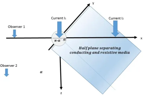
2. A simple 2D model with conducting sea represented

as a wedge

Figure 4. Model of the land/sea interface. The dipping plane with

slope α separates the conducting medium (sea) with resistivity 𝜌

to

the right from resistive medium with resistivity, 𝜌

to the left (land).

For the simple case the current

I

is injected at the origin with the

observer located on the x-axis on the land side. For the more

complicated case the current I

is injected into the sea along the x-axis

while the observer can be located at an arbitrary position on the

surface or inside the earth or inside the sea. Here we will only

consider the case where the observer is located in the resistive part.

2.1 The simple case

The model shown in Figure 4 was studied in the report for the simple

case. It is easy to show that for the simple case with current I

the

presence of the conducting sea changes the potential on the land side

by the factor (Rusck,1962)

𝜂 =

≅

,

where the approximate formula applies when the angle 𝛼 is small. The

effect of the sea it to conduct a relatively large proportion of the

current that is injected at the land-sea interface whereby the field on

the land side is reduced accordingly.

For the example shown in page 20, corresponding to the Forsmark

coast, 𝜌

is taken to be 10000 Ohm-m, 𝜌

to be 1.6 Ohm-m and the

slope α to be 0,001. These values seem to be realistic for the Forsmark

SSM 2016:05 ₂₆

case and the potential and electric fields on the land side shown in

Figures 1 and 2 should then be reduced by a factor

𝜂 =

10000 1.6 +1

=0.32

i.e. a reduction by approximately one third of the field and potential

that would have existed without the sea.

If the electrode is located in deeper water and the corresponding slope

of the water/sea bottom interface would be a factor of 10 higher than

in the case above, then the reduction in voltage observed on the land

side would be

𝜂 =

=0.032

The advanced case

It is interesting to note that in the more advanced case where the

current injection takes place in the ocean and the observer is located at

an arbitrary position on the land side an analytic (referred to in the

report as mathematical) solution exist, that dates back to an old paper

by Maeda (1955) and implemented numerically more recently by

Hunt et al. (2001). The potential is represented as an infinite series

involving Legendre function with arguments related to the distance

between source point and observation point.

In general the reduction of the voltage on the land side would be

greater than when the source is located at the intersection point

because a larger proportion of the total current in the electrode would

be deflected in the direction of the conducting sea. However, still the

main factor controlling the reduction of the voltage on the land side is

expected to be slope of the water/sea bottom interface. The bulk

resistivity in the upper part of the crust is expected to be of the order

10000 Ohm-m or higher as measured in several boreholes in the

Forsmark area even though local smaller scale variations due to fluids

in fracture zones can cause the resistivity to drop considerably.

It is beyond the scope of this report to implement the analytic

expressions into a computer code. It is only noticed that an analytic

solution exists and it would have been interesting if the numerical

results calculated using a finite element code were tested against the

analytic results for exactly the same model. Furthermore it would be a

more challenging task for the FEM model to reproduce the potential

because currents parallel to conductivity gradients are more difficult

to model than when they are orthogonal like in the case when the

current is injected at land-sea interface.

2.2 Comparing with observations

In the report (page 16) it mentioned that recent measurements of the

voltage drop from the shoreline at Fågelsundet (2.3 km from the

electrode at sea) to a point 2.7 km further inland is 200 V when

V. This is in very good agreement the calculation shown in Figure 3,

when a reduction factor slightly smaller than 0.2 is used. The same

reduction factor predicts an electric field at the shoreline of about 0.2

V/m as can be deduced from Figure 2.

SSM 2016:05 ₂₈

2.2.1 Around Fågelsundet

In Figure 4-3 of the report the voltage distribution away from different

Scandinavian electrodes is shown (reprinted from Tykeson et al.

(1996). For the Fågelsundet electrode this the voltage drop over

approximately the same distance as above is about 5 V, 40 times

lower than the number quoted above. The disagreement between the

two measurements is striking. In the report it explained that the

Tykeson et al. measurements were made in the sea away from the

shore whereas the recent measurements were made on land away from

the shore. The authors explain this as a difference in setup: Difference

between Fenno-Skan 1 and 2 and difference in water temperature.

This difference could perhaps explain a factor of two difference

between the two meausrements, but not a factor 40. A more effective

way of reducing the voltage on the sea side is to increase the water

depth away from the electrode more than predicted by the small slope

of 0.001.

2.2.2 Around Forsmark

Forsmark is located around 25 km from the Fågelsundet. Looking at

Figure 2 and using a reduction factor of 2 we find an electric field

about 1.5 mV/m = 1.5 V/km. In the report, page 17 it is mentioned

that the local voltage at Forsmark is anticipated to be 0.5 V/m. It is not

clear how this figure was calculated, but presumably from a model of

the earth with a lower resistivity at greater depth than the standard

10000 Ohm-m that was used throughout in this appendix.

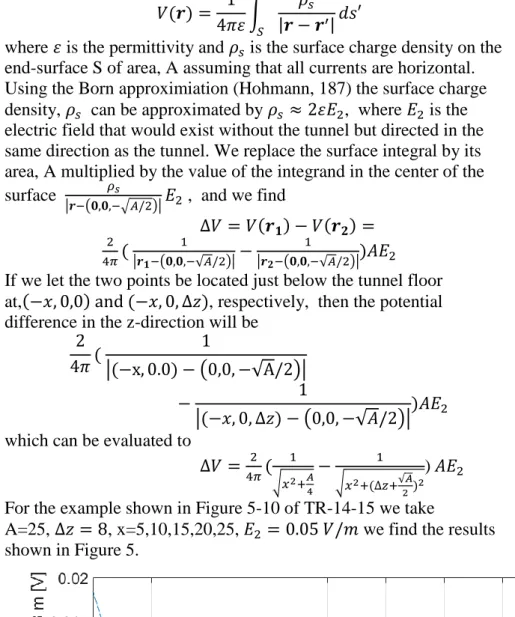
3. Approximate calculation of voltage drop around a

long tunnel filled with conductive material (bentonite

clay)

The large field strength calculated below the deposition holes in

Figure 5-12 in TR-14-15 is puzzling. The FEM calculations give an

average field strength of about 4/8 V/m= 500 V/km to be compared

with an impressed field of 50 V/km! It was therefore decided to take

an approximative approach to the problem resulting in an analytic

solution. Only one deposition tunnel was considered and the current

inside the tunnel was assumed to be horizontal.

Let a long tunnel filled with bentonite clay have a quadratic

cross-sectional area, A. Let the electrical conductivity of the clay be 𝜎

and

that of the surrounding rock be 𝜎

≪ 𝜎

. The tunnel is taken be

sufficiently long that the influence of the opposing ends can be

neglected when considering the potential close to the end face. The

end face is located at x=0 and let its center be located at

(x,y,z)=(0,0,-√𝐴) with the z-axis pointing downward. If it is assumed that the

electric field just outside of the tunnel is the same as it would be

without the tunnel we find for the potential 𝑉 = 𝑉(𝑥, 𝑦, 𝑧)

𝑉(𝒓) =

1

4𝜋𝜀

∫

𝜌

|𝒓 − 𝒓

_|

𝑑𝑠′

where 𝜀 is the permittivity and 𝜌

is the surface charge density on the

end-surface S of area, A assuming that all currents are horizontal.

Using the Born approximiation (Hohmann, 187) the surface charge

density, 𝜌

can be approximated by 𝜌

≈ 2𝜀𝐸

, where 𝐸

is the

electric field that would exist without the tunnel but directed in the

same direction as the tunnel. We replace the surface integral by its

area, A multiplied by the value of the integrand in the center of the

surface

𝐸

, and we find

∆𝑉 = 𝑉(𝒓

) − 𝑉(𝒓

) =

(

−

)𝐴𝐸

If we let the two points be located just below the tunnel floor

at,(−𝑥, 0,0) and (−𝑥, 0, ∆𝑧), respectively, then the potential

difference in the z-direction will be

2

4𝜋

(

1

|(−x, 0.0) − (0,0, −√A/2)|

−

1

|(−𝑥, 0, ∆𝑧) − (0,0, −√𝐴/2)|

)𝐴𝐸

which can be evaluated to

∆𝑉 =

(

−

) 𝐴𝐸

For the example shown in Figure 5-10 of TR-14-15 we take

A=25, ∆𝑧 = 8, x=5,10,15,20,25, 𝐸

= 0.05 𝑉/𝑚 we find the results

shown in Figure 5.

Figure 5. Approximate calculation of voltage drop over 8 m below

floor of deposition tunnel.

It is noticed that compared with the FEM calculation shown in Figure

5-12 of TR-14-15 there are two main differences. Firstly the level of

the voltage drop is about 1000 times larger for the FEM calculations.

Secondly the decay of the voltage away from the end face is much

smaller than the one calculated here. When part of the current in the

x-SSM 2016:05 ₃₀

closer to the end face it will give rise to larger vertical voltage

differences. Obviously the present model (so-called Born

approximation) for the calculation of the vertical voltage drop is too

simple in that currents are only allowed to flow in the horizontal

direction. However, this big difference in the voltage behavior is

intriguing, and is is recommended that an independent numerical

modelling exercise be made to control the FEM calculations.

4. Conductance of cylindrical shell

The conductance, C of a cylindrical shell with conductivity varying as

a function of distance is given by

𝐶 = (

𝐴𝑟𝑒𝑎

𝑙𝑒𝑛𝑔𝑡ℎ

∗ 𝑐𝑜𝑛𝑑𝑢𝑐𝑡𝑖𝑣𝑖𝑡𝑦) =

1

𝑙

∫ 𝜎(𝑟

_{)2𝜋𝑟′}

𝑑𝑟

_,

where l is the length of the cylinder and radii 𝑟

and 𝑟

denote the

inner and outer radius of the shell, respectively. 𝜎 is the electrical

conductivity.

Assuming that the conductivity is a linear function of the water

content, 𝑤(𝑟) we can write

𝜎 = 𝛼(𝑤 + 𝑤

),

and we find

𝐶 =

1

𝑙

∫ 𝛼(𝑤 + 𝑤

)2𝜋𝑟′

𝑑𝑟

=

𝑐

𝑙

∫ 𝑤2𝜋𝑟′

𝑑𝑟

+

𝛼

𝑙

∫ 𝑤

2𝜋𝑟

𝑑𝑟

=

𝛼

𝑙

𝑊 + 𝐶

,

where W is the total water content per unit length of the cylindrical

shell and 𝛼 and 𝐶

are experimental constants.

If the water is redistributed within the shell such that the total water

content is unchanged then the electrical conductance (inverse

resistance) is also unchanged.

5. References

Maeda, K., 1955. Apparent resistivity for dipping beds. Geophysics

20, 123-139.

Hohmann, G.W., 1987. Numerical modeling for electromagnetic

methods of geophysics. In Electromagnetic Methods in Applied

Geophysics, vol 1, Theory, edited by M.N. Nabighian, Society of

Exploration Geophysics, Tulsa, Oklahoma.

Hunt, P., N. Powell, K.A. Watson, 2001. Limiting apparent-resistivity

values for dipping-bed earth-models. Geophysical Prospecting 49,

577-591.

2016:05 The Swedish Radiation Safety Authority has a comprehensive responsibility to ensure that society is safe from the effects of radiation. The Authority works to achieve radiation safety in a number of areas: nuclear power, medical care as well as commercial products and services. The Authority also works to achieve protection from natural radiation and to increase the level of radiation safety internationally. The Swedish Radiation Safety Authority works proactively and preventively to protect people and the environment from the harmful effects of radiation, now and in the future. The Authority issues regulations and supervises compliance, while also supporting research, providing training and information, and issuing advice. Often, activities involving radiation require licences issued by the Authority. The Swedish Radiation Safety Authority maintains emergency preparedness around the clock with the aim of limiting the aftermath of radiation accidents and the unintentional spreading of radioactive substances. The Authority participates in international co-operation in order to promote radiation safety and finances projects aiming to raise the level of radiation safety in certain Eastern European countries.

The Authority reports to the Ministry of the Environment and has around 300 employees with competencies in the fields of engineering, natural and behavioural sciences, law, economics and communications. We have received quality, environmental and working environment certification.