LEVERAGING HIGH-RESOLUTION TRAFFIC DATA TO
UNDERSTAND THE IMPACTS OF CONGESTION ON SAFETY
Tingting Huang1, Shuo Wang2, Anuj Sharma3
1,2,3Department of Civil, Construction and Environmental Engineering, Iowa State University 1,2,32711 South Loop Dr., Suite 4700, Ames, Iowa, U.S.
1Phone: +1 402-499-6827 E-mail: thuang1@iastate.edu 2Phone: +1 402-570-3226 E-mail: shuowang@iastate.edu
3Phone: +1 402-472-6391 E-mail: anujs@iastate.edu
ABSTRACT
Since vehicle crashes in urban area may potentially cause higher societal costs than those in rural area, it is critical to understand the contributing factors of urban crashes, especially congestions. This paper analyzes the impacts of segment characteristics, traffic-related information and weather information on monthly crash frequency based on a case study in Iowa, U.S. Random parameter negative binomial (RPNB) model was employed. Considering that same factor may impact crash frequency differently on segments with different congestion level, the heterogeneity in random parameter means was introduced and discreetly examined. Data from 77 directional segments and 24 months (2013-2014) were used in this study. The empirical results show that segment length and maximum snow depth have fixed impacts while number of lanes, shoulder width and trailers percentage have random impacts on crash frequency. In addition, heterogeneous behaviors of the random factors were identified between segments with different congestion level. For example, the model results indicate that the increase of left shoulder width tends to decrease crash frequency more under congested condition than under uncongested condition.
1.
INTRODUCTION
Crashes on urban interstates may cause huge economic losses and societal impacts due to the property damage, personal injury, travel delay and other issues. According to the estimation by National Highway Traffic Safety Administration (NHTSA, 2014), interstate highway crashes caused $28 billion in economic costs and $88 billion in comprehensive costs in 2010 in the U.S. In order to reduce crashes and improve traffic safety, providing important insight of highway design and operation by estimating crash frequency is necessary.
Numerous research efforts have been made into understanding factors that contribute to traffic accidents, including highway crashes, intersection crashes and pedestrian crashes. These studies have introduced many statistical approaches to recognize significant factors that have impacts on crash frequency and severity. Lord and Mannering (2010) have summarized 16 types of models used in analyzing crash count data and assessed the advantages, disadvantages and applicability of each model. Several models related to this research will be reviewed and present in this paper.
Some significant factors impacting crash frequency have been identified in previous researches. The increase in segment length, curvature or annual average daily traffic (AADT) may increase crashes, meanwhile, the increase in sight distance, pavement friction and longitudinal slope may decrease crash frequency on a four-lane highway (Caliendo, C., 2007). Weather factors like annual average snowfall were also shown to have significant impacts on crashes (Ye, X., 2009). In light of the traffic condition on urban interstates, few studies have estimated the relationship between congestion and crash frequency. In this research, besides segment characteristics and weather information, an aggregated traffic performance measure describing monthly congestion level has been analyzed.
This study analyzes monthly crash counts using a random parameter negative binomial (RPNB) model. Different from traditional analysis about road geometry, traffic-related and weather information, this study also emphasizes on the impacts of congestion. Thus, the RPNB model also took the heterogeneity in random parameter means into account. Instead of directly using the congestion as an isolated variable, this study utilizes the congestion condition as the variable which may cause different behaviors of those road geometry, traffic-related and weather factors. The congestion is defined by the percentage of time when speed is less than monthly average speed by 25 mph. If the percentage is above the overall mean percentage, then this situation will be defined as congestion, and if the percentage is below the overall mean percentage, then it will be defined as non-congestion. This model was applied on the Interstate 235 (Des Moines, IA, U.S.) dataset which can reflect the urban interstate situation. The significant factors were found and interpreted by examining the model estimation results.
2.
LITERATURE REVIEW
The traditional Poisson model is considered as an elementary method to analyze count data, however, it has limitation in handling over-dispersion which is quite common in crash data. Miaou (1994) has evaluated the performance of Poisson and negative binomial (NB) model in estimating the relationship between truck crash and road geometric design. He recommended that NB model should be used when high over-dispersion (Wedderburn’s over-dispersion parameter>1.3) was found in crash data. Poch and Mannering (1996) also found that using Poisson instead of NB would have considerable bias in coefficient estimates when analyzing the intersection crash frequency. If the over-dispersion is not known beforehand, another more flexible model that could handle not only over-dispersion, but also under-dispersion, the generalized Poisson regression model can be used (Famoye, F., 2004). Due to the characteristics of traffic accident, the over-dispersion is shown in most crash count dataset and hence the NB model is a good fit in modeling crash frequency.
Since crash count data are usually characterized by considerable amount of zeros, some researchers also have used zero-inflated Poisson (ZIP) model or zero-inflated NB (ZINB) model to accommodate excessive zeros. Aguero-Valverde (2013) has employed the ZIP, ZINB and ZIP lognormal model in
analysis of crash count dataset and compared the accuracy with basic NB and Poisson lognormal model. The model results showed that ZI models had lower deviance than regular models. However, Lord (2007) also argued against the “pure zero” state generated by ZI model in traffic safety realm. Based on the characteristics of the dataset in this study, the ZI model was not adopted.
Another concern in modeling crash frequency is the unobserved heterogeneity in roadways. To capture the variation of effects caused by variables, many researchers chose random parameter (RP) model than fixed parameter model, and the former allowed parameters to vary across observations. Anastasopoulos and Mannering (2009) have used both fixed parameter model and RP model to identify the factors impacting crash frequency on rural interstates. They found that the increase in road segment length or AADT might increase the crash frequency; the increase in median width, shoulder width, or presence of median barriers decreased the number of crashes. And their impacts on crashes varied across segments. By comparing the predicted mean and the actual values for both models, it was presented that the RP model provided a better fit.
As the RP model has been in use widely recently, besides the unobserved heterogeneity, the heterogeneity in random parameter means has also been noticed. In several papers (Venkataraman, N. S., 2011, 2013, 2014), data were aggregated independently using four ways: type of interchange, severity, number of vehicle involved and crash type, and then estimated separately by using the heterogeneity-in-means RPNB model. The results showed that AADT, median continuation, largest degree of curvature and vertical curve gradient might have heterogeneous influence on crash frequency of roadway segments with different type of interchange due to the variation in random parameter means (Venkataraman, N. S., 2014). Analyzing the heterogeneity in means could help us to better understand some specific practical concern in traffic safety. To explicitly explore the different effects that factors may have on segments with different congestion condition, a RPNB model associated with heterogeneity-in-means approach has been considered in this study.
3.
METHODOLOGY
The NB model is a generalization of the Poisson model to handle the over-dispersion in crash frequency data. For the discrete random variable (monthly crash frequency) denoted as Y, observed frequencies denoted as yi (where i = 1, . . . , n; yi is a nonnegative integer count) and regressors xi, the basic Poisson
regression model is given by: Prob(Y = yi|xi) =
exp (−λi)λi𝑦𝑖
yi! , i = 1,2,3, … (1) where λi is both the mean and variance of monthly crash frequency, and the natural logarithm of λi is
modeled as below: log λi = β′x
i (2)
The NB model introduces an extra heterogeneity term εi to the estimated log λi and denotes a new term μi:
log μi = log λi+ εi= β′x
i+ εi (3)
where μi= exp(εi) λi is the new mean of monthly crash frequency; exp(εi) follows Gamma distribution
with mean equals to one and variance equals to α. Still assuming monthly crash frequency follows Poisson distribution with mean equals μi and simply replacing λi with μi= exp(εi) λi in basic Poisson
regression model, the NB model is derived: Prob(Y = yi|εi, xi) =
exp[−(exp(εi) λi)] [exp(εi) λi]yi
And the final form of NB model can be reduced as: Prob(Y = yi|xi) = Γ(θ + yi) Γ(θ)Γ(yi+ 1)uiθ(1 − ui)yi (5) where ui=θ+λθ i, θ = 1
α, α is the over-dispersion parameter. And the relationship between mean and
variance of modeled monthly crash frequency is given by:
Var[Y|εi, xi] = E[Y|εi, xi](1 + α) > E[Y|εi, xi] (6) With this property, NB model is a good fit for modeling the over-dispersed crash frequency data. The RP model was applied to allow the model parameters to vary among different segments to count for the unobserved heterogeneity. In addition, to examine the impact of speed conditions varying across segments and months, the heterogeneity-in-means approach in this model was introduced to allow the means of random parameters to vary among segments with or without congestion. In this heterogeneity-in-means RPNB model, λij is modeled as below:
log λij= β1′x1+ β2i′x2 (7) β2i′= β2+ Δ1z1+ vi (8) where i stands for the 𝑖𝑡ℎ segment; j stands for the 𝑗𝑡ℎ month; x
1 is a K1× 1 vector of observations for
nonrandom variables; x2 is a K2× 1 vector of observations for random variables; β1′ is a K1× 1 vector
of nonrandom parameters; β2i′ is a K2× 1 vector of random parameters for segment i (it only varies between different segments in the panel data set); β2 is a K2× 1 vector of fixed means of random parameter distributions; z1 is the value of congestion indicator and Δ1 is a K2× 1 vector of coefficients of congestion indicator, they form the segment specific term in the means caused by congestion; vi is
unobservable K2× 1 latent random term in the ith observation in β2i . In this research we assume each
element of vi follows normal distribution with zero mean.
If a variable xk is believed to be an exposure measure of crash frequency, this variable is treated as offset variable and the logarithm of this variable log (xk) is used in the count model as shown below (βk is the parameter of log (xk) and the other symbols are as defined before):
log λij= βklog (xk) + β1′x1+ β2i′x2 (9) λij= exp(βklog(xk) + β1′x1+ β2i′x2) = xkβkexp(β1′x1+ β2i′x2) (10)
βk is often preset to 1 so that the average monthly crash frequency λij is proportional to xk. If βk is not
restricted, it should be close to 1 to maintain the offset assumption.
All the parameters were considered to be random in the first place and then set to be fixed when both the heterogeneity-in-means and the scale parameter showed no significance at any reasonable confidence level. In order to estimate the unobserved heterogeneity across different segments, the constant term was always kept random.
To infer the heterogeneity in means for each random parameter, a feasible way is calculating the percentage of positive in parameter distributions which may vary among congested and uncongested segments (12):
𝑃+𝛽 = ∫0+∞ϕ𝛽(x)dx (11) 𝑃+𝛽 indicates what percentages of road segments have potentially more crashes when the variable is
decided by the parameter distribution which is usually described by statistics (mean and standard deviation), so the heterogeneity in means will be directly reflected in the differences of 𝑃+𝛽 under
different situations.
Simulated maximum likelihood method was employed in the model fitting process. The Broyden– Fletcher–Goldfarb–Shanno algorithm was utilized to search the optimal parameters iteratively (NLOGIT, 2007). For the coefficient estimation in each iteration, Halton draw was used instead of random draw to speed up the convergence (Halton, J., 1996). Previous research has shown that 100 Halton draws is usually sufficient (Bhat, C., 2003)so 100 Halton draws was used in this study. All the process was conducted in NLOGIT.
4.
DATA OVERVIEW
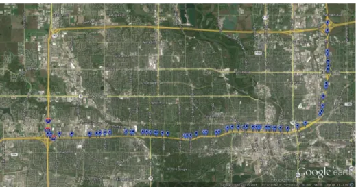
The data consisted of roadway characteristics, monthly traffic speed measures and monthly weather statistics. There were 492 crashes on I-235 through lanes during the study period. The study road is a 13.8-mile-long urban freeway. The roadway geometric information and AADT by vehicle types were provided by Iowa Department of Transportation from Geographic Information Management System. In this system, every time the roadway geometric attributes (e.g. number of lanes) changed the road was divided into segments at that point and finally the study road was divided into 384 small directional segments with 385 feet average length. To avoid excessive zeros that might be generated by such short segments, the adjacent, homogenous, small segments have been grouped into one longer segment with length-weighted geometric and volume information. Then, a total of 77 directional segments have been created with 1853 feet average length (shown in Figure 1).
Figure 1: Locations of segments in study area (blue pins).
Historical monthly weather data were extracted from Quality Controlled Local Climatological Data in National Climatic Data Center. Since the Des Moines airport weather station is the only station in study area and 3.67mi to 8.82 mi away from studied corridor, monthly weather reports for this station were obtained and the potentially effective weather variables were extracted. All the 77 segments share the same weather information so the weather variables are only time-variant.
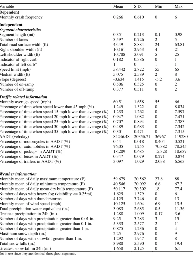
The archived traffic speed data in 1-min interval were obtained from INRIX and traffic speed measures were computed at monthly aggregation level. The percentage of time with average speed less than 45 mph (generally considered as congestion on interstates) and percentages of time with speed 15/20/25/30/35 mph less than average speed have been conducted to evaluated different congestion levels. In Table 1, “Percentage of time when speed lower than” variables are describing the certain levels of congestion happened during a month on one segment.
After combining segment characteristics, traffic-related and weather information, 40 variables in total were examined to model segment monthly crash frequency. The descriptive statistics of all the variables are shown in Table 1.
Table 1: Descriptive Statistics of Variables.
Variable Mean S.D. Min Max
Dependent
Monthly crash frequency 0.266 0.610 0 6
Independent
Segment characteristics
Segment length (mi) 0.351 0.213 0.1 0.98
Number of lanes 3.597 0.726 2 5
Total road surface width (ft) 43.49 8.884 24 63.81
Right shoulder width (ft) 10.161 2.953 4 21
Left shoulder width (ft) 10.788 3.091 5 25
Indicator of right curb 0.182 0.386 0 1
Indicator of left curb* 1 0 1 1
Speed limit (mph) 58.442 2.822 55 65
Median width (ft) 5.075 2.589 2 8
Slope (degrees) -0.634 1.415 -5.2 3.6
Number of on-ramp 0.506 0.525 0 2
Number of off-ramp 0.377 0.511 0 2
Traffic related information
Monthly average speed (mph) 60.51 1.658 55 66
Percentage of time when speed lower than 45 mph (%) 1.249 1.322 0 8.034
Percentage of time when speed 15 mph lower than average (%) 1.233 1.262 0 7.597
Percentage of time when speed 20 mph lower than average (%) 0.947 1.082 0 7.471
Percentage of time when speed 25 mph lower than average (%) 0.707 0.894 0 7.383
Percentage of time when speed 30 mph lower than average (%) 0.489 0.683 0 7.342
Percentage of time when speed 35 mph lower than average (%) 0.301 0.471 0 7.315
AADT (veh/day) 84246.48 20356.71 36967 119280
Percentage of motorcycles in AADT (%) 0.44 0.018 0.404 0.521
Percentage of automobiles in AADT (%) 76.05 1.255 70.382 78.545
Percentage of pickups in AADT (%) 18.209 0.685 15.328 18.637
Percentage of buses in AADT (%) 0.347 0.079 0.271 0.874
Percentage of trailers in AADT (%) 3.097 1.029 2.038 6.563
Weather information
Monthly mean of daily maximum temperature (F) 59.679 20.562 27.8 88
Monthly mean of daily minimum temperature (F) 40.546 20.092 6.6 67.2
Monthly mean of daily mean dry bulb temperature (F) 50.117 20.302 18 77.4
Number of days with heavy fog (visibility <= 0.25mi) 1.625 1.379 0 6
Number of days with thunderstorms 4.125 3.746 0 13
Monthly mean of wind speed (mph) 10.125 1.604 6.9 13.5
Total precipitation water equivalent (in.) 3.083 2.685 0.5 11.36
Greatest precipitation in 24h (in.) 1.288 1.009 0.17 3.6
Number of days with precipitation greater than 0.01 in. 9.25 3.283 3 15
Number of days with precipitation greater than 0.1 in. 5.333 2.577 2 11
Number of days with precipitation greater than 1 in. 0.875 1.236 0 4
Maximum snow depth (in.) 2.25 2.976 0 9
Number of days with snowfall greater than 1 in. 1.292 1.947 0 8
Total snow falls (in.) 3.988 5.590 0 19.4
Greatest snow fall in 24h (in.) 1.658 2.125 0 6.1
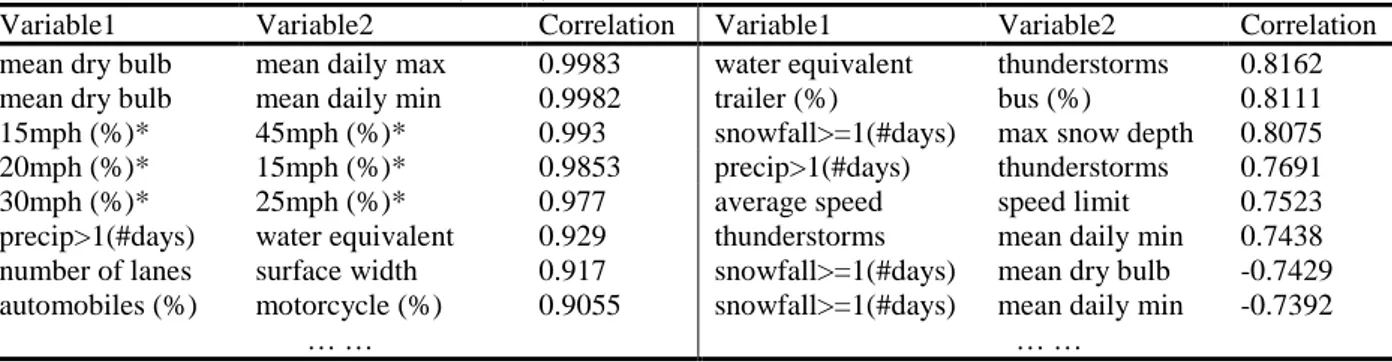
Out of 40 variables, there are 25 variables which have strong correlations (>0.7 or <-0.7) with each other. Most variables in terms of weather information are correlated. Some traffic condition related variables, such as percentage of time when speed 15 mph lower than average and percentage of automobiles in AADT are correlated to other speed or volume variables due to the inherent relationship among them. The pairwise correlations between variables are partially shown in Table 2.
Table 2: Pairwise Correlation in Variables (Partial).
Variable1 Variable2 Correlation Variable1 Variable2 Correlation
mean dry bulb mean daily max 0.9983 water equivalent thunderstorms 0.8162
mean dry bulb mean daily min 0.9982 trailer (%) bus (%) 0.8111
15mph (%)* 45mph (%)* 0.993 snowfall>=1(#days) max snow depth 0.8075
20mph (%)* 15mph (%)* 0.9853 precip>1(#days) thunderstorms 0.7691
30mph (%)* 25mph (%)* 0.977 average speed speed limit 0.7523
precip>1(#days) water equivalent 0.929 thunderstorms mean daily min 0.7438
number of lanes surface width 0.917 snowfall>=1(#days) mean dry bulb -0.7429
automobiles (%) motorcycle (%) 0.9055 snowfall>=1(#days) mean daily min -0.7392
… … … …
* short for those speed related variables
Strong correlations among variables should be avoided in model estimation due to the increased standard error caused by those variables. By eliminating those 25 variables, the remaining 15 variables (Table 3) can be input into the regression procedure.
Table 3: Input Variable.
Segment Characteristics Traffic Related Information Weather Information
Segment length Slope AADT Maximum snow depth
Number of lanes Indicator of right curb Percentage of trailers Monthly mean of wind speed
Median width Number of on-ramp Percentage of time when
speed 25 mph lower than average speed (“P25”)
Number of days with heavy fog
Right shoulder width
Number of off-ramp Left shoulder width
Plus, in order to capture the heterogeneity in means caused by congestion, a congestion indicator has been created by coding “P25” variable into 0 (non-congestion) when it is less than average “P25”, otherwise, into 1 (congestion).
5.
MODEL ESTIMATION
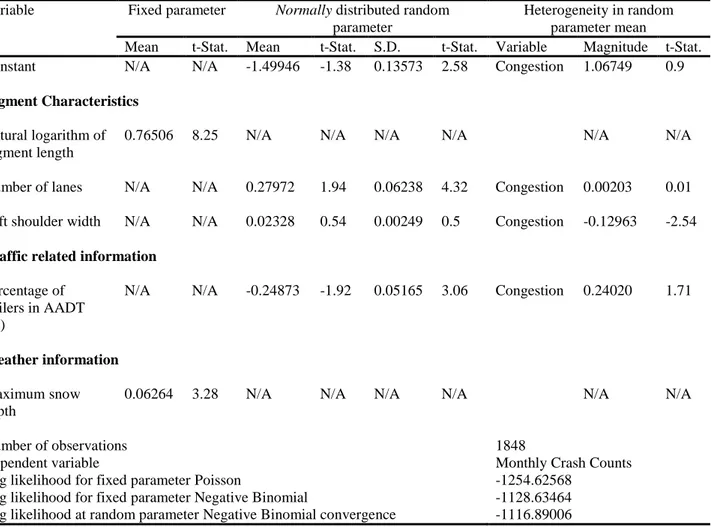
This study used the RPNB model to estimate the parameters from 1848 observations. The final model estimation results are shown in Table 4.
Table 4: Heterogeneity-In-Means Random Parameter Negative Binomial Model Estimation Results.
Variable Fixed parameter Normally distributed random
parameter
Heterogeneity in random parameter mean
Mean t-Stat. Mean t-Stat. S.D. t-Stat. Variable Magnitude t-Stat.
Constant N/A N/A -1.49946 -1.38 0.13573 2.58 Congestion 1.06749 0.9
Segment Characteristics Natural logarithm of segment length
0.76506 8.25 N/A N/A N/A N/A N/A N/A
Number of lanes N/A N/A 0.27972 1.94 0.06238 4.32 Congestion 0.00203 0.01
Left shoulder width N/A N/A 0.02328 0.54 0.00249 0.5 Congestion -0.12963 -2.54
Traffic related information Percentage of
trailers in AADT (%)
N/A N/A -0.24873 -1.92 0.05165 3.06 Congestion 0.24020 1.71
Weather information Maximum snow depth
0.06264 3.28 N/A N/A N/A N/A N/A N/A
Number of observations 1848
Dependent variable Monthly Crash Counts
Log likelihood for fixed parameter Poisson -1254.62568
Log likelihood for fixed parameter Negative Binomial -1128.63464
Log likelihood at random parameter Negative Binomial convergence -1116.89006
The log-likelihood value improved from fixed parameter Poisson model (-1254.62568), fixed parameter NB model (-1128.63464) to the final RPNB model (-1116.89006) which indicates the improvement of model goodness of fit.
Besides log-likelihood, other goodness of fit statistics have also been employed. Table 5 shows the mean absolute deviance (MAD) and mean squared predictive error (MSPE) (Oh et al, 2003) for RPNB model, fixed parameter NB model and fixed parameter Poisson model.
Table 5: Goodness of Fit Statistics.
RPNB model Fixed Parameter NB model Fixed Parameter Poisson model
Log-likelihood -1116.89006 -1128.63464 -1254.62568
MAD 0.3722 0.3896 0.3943
MSPE 0.3211 0.3397 0.3450
Table 5 shows the RPNB model has lower MAD and MSPE value than other two models, which indicates the better fit of RPNB model.
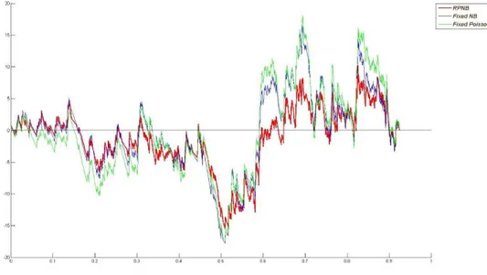
A variable-based cumulative residual (CURE) plot (Hauer, 2015) was also used to assess the goodness of fit (shown in Figure 2). The CURE plot presents how the models fit the data by examining if the cumulative residuals oscillate around zero for the interested variable (Geedipally et al, 2010).
Figure 2: Adjusted CURE Plot for Segment Length Variable.
Figure 2 shows the CURE plot for segment length variable. This figure was adjusted to make final value equal to zero (Geedipally et al, 2012). The RPNB model curve is closer to zero comparing with fixed parameter models which shows that RPNB model fits the data better.
6.
RESULTS INTERPRETATION
As shown by parameter estimation, constant term was found to be random with significant standard deviation of the parameter distribution. It means extra heterogeneity was not captured by the explanatory variables in the final model but only handled by the random constant term.
In order to interpret heterogeneity in means caused by congestion, percentage of positive in parameter distribution has been computed by employing equation (11), and results are shown in Table 6.
Table 6: Percentage of Positive in Parameter Distribution.
Variable Parameter Distribution under Non-congestion Parameter Distribution under Congestion
Mean S.D. % of Positive % of Negative Mean S.D. % of Positive % of Negative Number of lanes* 0.27972 0.06238 ~100 ~0 0.28175 0.06238 ~100 ~0
Left shoulder width 0.02328 0.00249 ~100 ~0 -0.10635 0.00249 ~0 ~100
Percentage of trailers
in AADT (%) -0.24873 0.05165 ~0 ~100 -0.00853 0.05165 43.441 56.559
* not significant in heterogeneity in mean
From Table 4 and Table 6, it can be found that left shoulder width and trailers percentage behave significantly differently when congestion occurs. Further discussion of all the critical variables are shown below.
Since crash frequency is supposed to increase on longer segment, segment length was treated as offset variable (a measure of exposure) and the natural logarithm of segment length was used in the model. The estimated parameter of logarithm of segment length is 0.76506 which is a little lower than 1. That indicates the crash frequency is near proportional to segment length and with the increase in segment length, the increase in crash frequency slightly decreases.
As number of lanes may account for more latent traffic flow variabilities, it shows more impacts on crash frequency and was picked by the model. As a random parameter, number of lanes does not show strong statistical significance in heterogeneity in means caused by congestion. The positive sign of estimated mean indicates that crashes may increase as number of lanes increases in both congested and
uncongested segments. This result is consistent with some previous research. Milton (1998) and Abdel-Aty (2000) found number of lanes and crash rates have positive relations.
Left shoulder width was identified to have statistical significance regarding the heterogeneity in parameter mean caused by congestion. For uncongested situation, the estimated mean is not statistical significant. However, when congestion happens, the estimated mean is negative, which means almost 100% segments may have lower crash frequency with wider left shoulder. This is consistent with the previous findings about left shoulder width by Fitzpatrick (2008). In addition, it is also intuitively reasonable to assume that better lateral clearance helps reduce crashes.
The sign of parameter for trailers percentage is negative for almost 100% segments which are uncongested. While when congestion occurs, on near 43% segments, the impact of trailers will be shifted to “positive” impact, which means the higher percentage of trailers is, the more crashes may be expected. This contradictory impact may due to the different data aggregation level. The crash and speed information were aggregated at monthly level, however, trailers percentage was aggregated at annual level which may not perfectly represent monthly traffic flow situation.
For weather information, only maximum snow depth showed significant impact on crashes. The parameter for maximum snow depth is fixed because all the segments share the same weather information. The positive mean 0.06264 indicates as more snow falls at a time, more crashes are expected to occur.
7.
SUMMARY AND CONCLUSIONS
This paper demonstrated an application of heterogeneity-in-means RPNB model to analyze the key factors impacting monthly crash frequency on urban interstate. The RPNB model can better estimate over-dispersed data than traditional Poisson model and capture the unobserved heterogeneity by allowing parameters to vary across segments. To understand the situation on urban interstates, congestion was chosen to be a main concern to explore the heterogeneous behavior other factors may exhibit. A heterogeneity-in-means approach was utilized in parameter estimation associated with RPNB model.
The data from 77 segments of 1-235 corridor during 2 years (2013-2014) was treated as panel data in this study. Segment characteristics, traffic-related information and weather information were contained in the dataset and processed as 40 independent variables. The final model showed that 5 variables were identified having significant impacts (fixed or random) on dependent variable. Analyzed by model estimation, segment characteristic factors (natural logarithm of segment length, left shoulder width and number of lanes), traffic-related factor (percentage of trailers in AADT) and weather factor (maximum snow depth) are statistically significant in impacting on monthly crash frequency. In these factors, segment length and maximum snow depth have fixed parameter. While number of lanes, left shoulder width and trailers percentage have random parameter that make their impacts vary across segments. In terms of congestion, factors with random parameter have heterogeneous impacts on crash between congested and uncongested segments.
This exploratory study provides an insight of critical factors impacting crash frequency, especially focusing on congestion level which derived from high-resolution speed data. Since this study only has 77 segments as objects, a larger sample is still expected in order to expand the knowledge of urban interstate safety.
REFERENCES
Abdel-Aty, M. A., and A. E. Radwan. (2000). Modeling Traffic Accident Occurrence and Involvement. Accident Analysis and Prevention, Vol. 32(5), pp. 633–642.
Aguero-Valverde, J. (2013). Full Bayes Poisson Gamma, Poisson Lognormal, and Zero Inflated Random Effects Models: Comparing the Precision of Crash Frequency Estimates. Accident Analysis & Prevention, Vol. 50, pp. 289-297.
Anastasopoulos, P. C., and F. L. Mannering. (2009). A Note on Modeling Vehicle Accident Frequencies with Random-Parameters Count Models. Accident Analysis & Prevention, Vol. 41(1), pp. 153-159. Bhat, C. (2003). Simulation Estimation of Mixed Discrete Choice Models Using Randomized and Scrambled Halton Sequences. Transportation Research Part B: Methodological, Vol. 37(1), pp. 837– 855.
Caliendo, C., M. Guida, and A. Parisi. (2007). A Crash-Prediction Model for Multilane Roads. Accident Analysis & Prevention, Vol. 39(4), pp. 657-670.
Famoye, F., J. T. Wulu, and K. P. Singh. (2004). On the Generalized Poisson Regression Model with an Application to Accident Data. Journal of Data Science 2, pp. 287-295.
Fitzpatrick, K., D. Lord, and B. Park. (2008). Accident Modification Factors for Medians on Freeways and Multilane Highways in Texas. Transportation Research Record: Journal of the Transportation Research Board, Vol. 2083, pp. 62–71.
Geedipally, S. R., S. Patil, D. Lord. (2010). Examination of Methods for Estimating Crash Counts According to Their Collision Type. Transportation Research Record, Vol. 2165, pp. 12-20.
Geedipally, S. R., D. Lord, and S. S. Dhavala. (2012). The Negative Binomial-Lindley Generalized Linear Model: Characteristics and Application Using Crash Data. Accident Analysis & Prevention, Vol. 45, pp. 258-265.
Halton, J. (1996). On the Efficiency of Evaluating Certain Quasi-Random Sequences of Points in Evaluating Multi-Dimensional Integrals. Numerische Mathematik, Vol. 2(1), pp. 84–90.
Hauer, E. (2015). The Art of Regression Modeling in Road Safety. pp. 99-104.
NHTSA. (2014). The Economic and Societal Impact of Motor Vehicle Crashes, 2010. National Highway Traffic Safety Administration, Publication DOT HS 812 013, Washington, D.C.
Lord, D., and F. Mannering. (2010). The Statistical analysis of crash-frequency data: A Review and Assessment of Methodological Alternatives. Transportation Research Part A: Policy and Practice, Vol. 44(5), pp. 291-305.
Lord, D., S. Washington, and J. N. Ivan. Further Notes on the Application of Zero-Inflated Models in Highway Safety. Accident Analysis & Prevention, Vol. 39(1), 2007, pp. 53-57.
Miaou, S. (1994). The Relationship between Truck Accidents and Geometric Design of Road Sections: Poisson versus Negative Binomial Regressions. Accident Analysis & Prevention, Vol. 26(4), pp. 471-482.
Milton, J., and F. L. Mannering. (1998). The Relationship among Highway Geometries, Traffic-Related Elements and Motor-Vehicle Accident Frequencies. Transportation, Vol. 25(4), pp. 395–413.
Oh, J., C. Lyon, S.P. Washington, B.N. Persaud, and J. Bared. Validation of the FHWA Crash Models for Rural Intersections: Lessons Learned. In Transportation Research Record: Journal of the Transportation Research Board, No. 1840, Transportation Research Board of the National Academies, Washington, D.C., 2003, pp. 41-49.
Poch, M., and F. Mannering. (1996). Negative Binomial Analysis of Intersection-Accident Frequencies. Journal of Transportation Engineering, Vol. 122(2), pp. 105-113.
Venkataraman, N. S., and V. Shanker. (2014). A Heterogeneity-in-Means Count Model for Evaluating the Effects of Interchange Type on Heterogeneous Influences of Interstate Geometrics on Cash Frequencies. Analytic Methods in Accident Research, Vol. 2, pp. 12-20.
Venkataraman, N. S., G. F. Ulfarsson, and V. N. Shankar. (2013). Random Parameter Models of Interstate Crash Frequencies by Severity, Number of Vehicles Involved, Collision and Location type. Accident Analysis & Prevention, Vol. 59, pp. 309-318.
Venkataraman, N. S., et al. (2011). Model of Relationship between Interstate Crash Occurrence and Geometrics. Transportation Research Record: Journal of the Transportation Research Board, Vol. 2236.1, pp. 41-48.
Ye, X., et al. (2009). A Simultaneous Equations Model of Crash Frequency by Collision Type for Rural Intersections. Safety Science, Vol. 47(3), pp. 443-452.