Temperature-Gradient-Based Burn-In and Test
Scheduling for 3-D Stacked ICs
Nima Aghaee, Zebo Peng and Petru Eles
Linköping University Post Print
N.B.: When citing this work, cite the original article.
©2015 IEEE. Personal use of this material is permitted. However, permission to
reprint/republish this material for advertising or promotional purposes or for creating new
collective works for resale or redistribution to servers or lists, or to reuse any copyrighted
component of this work in other works must be obtained from the IEEE.
Nima Aghaee, Zebo Peng and Petru Eles, Temperature-Gradient-Based Burn-In and Test
Scheduling for 3-D Stacked ICs, 2015, IEEE Transactions on Very Large Scale Integration
(vlsi) Systems, (23), 12, 2992-3005.
http://dx.doi.org/10.1109/TVLSI.2014.2380477
Postprint available at: Linköping University Electronic Press
Abstract—Large temperature gradients exacerbate various types of defects including early-life failures and delay faults. Efficient detection of these defects requires that burn-in and test for delay faults, respectively, are performed when temperature gradients with proper magnitudes are enforced on an Integrated Circuit (IC). This issue is much more important for 3D stacked ICs compared with 2D ICs because of the larger temperature gradients in 3D stacked ICs. In this paper, two methods to efficiently enforce the specified temperature gradients on the IC, for burn-in and delay-fault test, are proposed. The specified temperature gradients are enforced by applying high power stimuli to the cores of the IC under test through the test access mechanism. Therefore, no external heating mechanism is required. The tests, high power stimuli, and cooling intervals are scheduled together based on temperature simulations so that the desired temperature gradients are rapidly enforced. The schedule generation is guided by functions derived from a set of thermal equations. Experimental results demonstrate the efficiency of the proposed methods.
Index Terms—3D Stacked IC test, burn-in, temperature gradients, test scheduling
I. INTRODUCTION
arge temperature gradients (e. g., temperature difference between two adjacent cores) exacerbate various types of defects including early-life failures and delay faults. The capability to detect these temperature-gradient induced defects is crucial for many ICs. In particular, three dimensional ICs exhibit considerably larger temperature gradients compared with normal ICs (for example, three times is reported in [29]) and therefore temperature-gradient based test is necessary for them.
A promising technology for fabricating 3D ICs is based on Through-Silicon Vias (TSV) used for inter-die connections [11], [13], [17], [27]. The ICs fabricated using TSVs are commonly referred to as 3D Stacked IC (3D-SIC) [17]. The important advantages of this technology include high inter-die interconnect densities and low inter-die interconnect wire lengths. This leads to higher operating frequencies at lower power consumptions.
A. Test for Early-Life Failures
Burn-in is a common way of accelerating and detecting early-life failures and it should be done with low cost in a reasonably short time. For this purpose, usually the dies are operated at elevated temperature and voltage. The elevated temperature and voltage speed up the aging and wear mechanisms so that the dies experience their early life before testing. The wear mechanisms that are speeded up include metal stress voiding and electromigration, metal slivers bridging shorts, as well as gate-oxide wear-out and breakdown [23].
Recently, several studies have, however, shown that some wear mechanisms are speeded up more efficiently by large temperature gradients rather than the high temperature itself. A temperature-gradient induced wear mechanism is identified in [25] which shows that a metal layer elevation develops rapidly on the sites that experience large temperature gradients. Moreover, in the atomic flux equation that models the electromigration, temperature gradient is present directly and also indirectly through its effect on the mechanical-stress gradient [21]. Therefore, a burn-in process that has not created the appropriate thermal scenarios does not sufficiently speed up the formation of the defects and, consequently, such early-life defects will go undetected. In order to prevent these test escapes, it is necessary to introduce a burn-in process that enforces appropriate temperature scenarios on the IC. This necessity is more urgent for the ICs that suffer from large temperature gradients, such as 3D-SIC.
3D-SIC technology, similar to other deep submicron technologies, suffers from high power densities. Additionally, power densities are considerably higher in the test mode compared to the functional mode, in particular for core-based designs [6], [33]. Consequently overheating may damage the ICs under test [2], [19], [32]. This means that the application of test stimuli to ICs can raise their temperatures beyond their tolerable limits. This often undesirable effect is, however, utilized in this paper to heat up the IC for burn-in. In our case the stimuli are not necessarily actual test patterns. Instead, they could be specially generated sequences which cause large switching activities. Such stimuli are called heating sequences. The use of the heating sequences to heat up the IC from inside means that special equipment for heating the IC from outside are not necessary. This will lead to large reduction of cost, and also allow for the generation of needed temperature gradients.
Some temperature gradients might be enforced on an IC by applying appropriate inputs to the IC’s input ports in the functional mode. This might work, to some extent, for 2D ICs, since from the functional point of view all the required circuitry, including the input ports, are there when the IC enters the test process. For 2D ICs, there are usually two possible stages for burn-in: Wafer-Level Burn-In (WLBI) which is performed before packaging and Die-Level Burn-In (DLBI) performed after packaging [23]. For 3D-SIC, there are more stages, including pre-bond, mid-bond, post-bond, and final stages [26]. At different stages, different defects can be targeted, based on their likelihood and considering the corresponding burn-in costs. A 3D-SIC, in addition to the defects that also exist for 2D, is affected by TSV related defects (e.g., defects related to TSV bonding). Such defects motivate, among other reasons, the use of these extra stages.
Existence of the test stages before the IC is fully assembled is a key difference between the 2D and 3D-SIC burn-in process. In the case of 3D-SIC, using input ports in the functional mode
Nima Aghaee, Zebo Peng, and Petru Eles
Temperature-Gradient Based Burn-In and
Test Scheduling for 3D Stacked ICs
may benefit burn-in for the post-bond and the final stages similar to 2D ICs. But for the pre-bond or mid-bond stages, the inputs to the die or partially stacked dies are not necessarily the inputs to the IC. The input ports to the unit under test for 3D-SICs, before the final bonding, are likely to include a number of TSVs. The TSVs and test equipment are not designed to support simultaneous application of functional signals, particularly to large number of TSVs (even though they might be designed to allow simple electrical tests for the TSV itself). Therefore, the use of the IC’s ports for enforcing the temperature gradients is not possible for the pre-bond and mid-bond stages. Albeit this lack of access in the functional mode, the Test Access Mechanism (TAM) provides access to the cores, in the test mode [1]. Therefore, the heating sequences could be applies using the TAM in order to enforce the desired gradients.
B. Test for Delay Faults
3D-SIC and other deep submicron technologies suffer from a considerably larger number of delay faults as compared with previous technologies. The causes for these delay faults include resistive bridges and vias, power droops, and cross-talk noise effects [5]. Therefore, delay-fault testing is necessary to provide sufficient fault coverage [14]. A large number of pre-bond TSV defects are resistive in nature and, moreover, the mechanical stress caused by TSVs contributes also to delay faults [11], [13]. Therefore, the expected number of delay faults for 3D-SIC is larger than that of 2D ICs.
Since temperature has a significant effect on delay, its impact should be taken into account for delay-fault test. A very important effect of temperature on signal integrity is its effect on the clock network [8]. Delay faults usually occur because of increased clock skew and a major contributor to skew in 3D-SICs is temperature gradient [20]. Since propagation delays depend on temperature, different temperatures on different sites (i.e., temperature gradients) result in clock skew. Temperature gradients may reach up to 50℃ in adjacent cores for normal operation and even higher during test [7], [8], [20]. Besides, as mentioned before, the temperature gradients in 3D-SICs are much larger than in 2D ICs [29]. This will exacerbate temperature-gradient related issues including delay faults, in particular, for 3D-SIC. Therefore, the associated tests should be performed when the proper temperature maps are enforced. A temperature map specifies the appropriate temperatures for different sites (e.g., cores) in the IC. These temperatures are to be realized simultaneously in order to enforce the proper temperature gradients. The temperature maps are given along with their corresponding tests. Beside the gradient-based burn-in (discussed burn-in section I.A) the other objective of this paper is to introduce a technique to apply the tests while the corresponding maps are enforced on the IC.
II. RELATED WORKS
Traditionally, burn-in is performed at elevated temperature, which is achieved by special equipment (e.g., temperature chambers) [23]. A more elaborate technique is a hybrid burn-in and test technique that provides tighter temperature control using an active heat-sink, without using temperature chambers [18]. These existing techniques are not able to enforce the specified temperature gradients, especially those with large magnitudes.
Despite the fact that enforcing specific temperature gradients will facilitate the detection of delay-faults, existing methods for delay-fault testing focus only on performing the tests disregarding the temperature gradients [5]. Apart from gradients, creating and maintaining some other kinds of thermal conditions during the test has been addressed previously. These existing techniques are briefly reviewed in the following.
A thermal-aware test scheduling is introduced in [30] for stacked multi-chip modules. The method tries to achieve a vertical uniform temperature distribution throughout the 3D-SIC during the test. The method is based on analytical simplifications of the temperature model [30].
A linear programming approach is used in [19] in order to generate thermally-safe test schedules for 3D-SICs. The proposed method uses a super-position based temperature simulator [19].
Two different approaches for multi-core ICs are introduced in [15] and [31] to guarantee that the cores’ temperatures are kept within the specified range when the corresponding tests are being applied. They focus on the temperature of the individual cores that are under test and the temperatures of other cores are neglected. Keeping the temperatures within the specified range is achieved by introducing heating sequences (high-power stimuli are applied) and cooling intervals (no stimuli are applied) into the test schedule.
Speeding up the test while minimizing the damages caused by overheating due to process variation is addressed in [2]. The test temperatures are kept sufficiently low by introducing cooling cycles. A number of test schedules are generated for different variation scenarios. During the test the proper schedule is selected based on the on-chip temperature sensor readouts (adapting to the current thermal variation situation). A fast temperature simulation technique that isolates heavy computations into a single initial phase is also suggested in [2]. The existing methods for controlling the chips’ temperatures during test try to respect a global upper temperature limit to prevent overheating [19], [32] or to respect upper and lower bounds for individual cores in order to target temperature dependent defects [15], [31]. In both cases, the temperature bounds are defined for each core independent from other cores and therefore spatial temperature gradients cannot be enforced. The first proposals to consider temperature-gradients in the burn-in and delay-fault test processes were made by us in [4] and [3], respectively, where the concept of temperature maps were introduced. Preliminary sketches of two simple algorithms to consider such temperature maps for burn-in and delay-fault test, respectively, were reported in [4] and [3]. This paper has built on the preliminary results of [3] and [4] and develops an integrated and systematic framework to address temperature-gradient issues in both burn-in and test processes. It presents also several advanced techniques to compute proper values for the test schedule’s period, to order the temperature maps, and to generate high-quality temperature-gradient based burn-in solutions, which were outside the scope of [3] and [4].
The rest of the paper is organized as follows. Section III addresses the temperature-gradient based burn-in. Section IV addresses temperature-gradient based test. Section V suggests an efficient temperature map ordering technique. Section VI presents experimental results. Section VII concludes the paper.
III. TEMPERATURE-GRADIENT BASED BURN-IN
A. Preliminaries and Problem Formulation
As discussed earlier, a temperature map specifies the desired temperature values for different sites (e.g., cores) in an IC. The temperature maps are to be given by the user, who studies the typical temperature-gradient induced failure mechanisms analytically or experimentally [21], [25]. Each map corresponds to a particular temperature condition of an IC, such as large temperature differences between adjacent cores (i.e., large temperature gradients), that can accelerate aging for early-life failures or enlarge the delay fault effect so that they can easily be tested for. There might also be some sites that their temperatures are not important regarding the targeted defects. Such sites are indicated as don’t-cares. Even though they are marked as don’t-cares, their temperature should, however, be kept below the overheating limit (denoted by 𝜃𝑜𝑣𝑒𝑟ℎ𝑒𝑎𝑡𝑖𝑛𝑔) in order to prevent damage.
When the expected locations in the IC simultaneously have the temperature values that are specified by a map, it is said that that temperature map is enforced. The specified temperature maps should be enforced quickly. In case of burn-in, the temperatures should then be enforced for a given period of time to achieve the intended effect. In case of test, a map should be enforced as long as the corresponding tests are being applied. Usually, there are many temperature maps that, therefore, it is important to enforce them rapidly whether the ICs start from the ambient temperature or from another map. The order of the maps has a considerable impact on the overall burn-in/test time, as will be discussed in section V. For the time being, we assume that the maps order is given and focus on other aspects of the problem. In our work, a temperature map will be enforced by applying heating sequences sent through the TAM. Moreover, it is assumed that no test is applied when an IC is kept under a temperature map for burn-in. This will be relaxed in section IV so that the tests can be applied when a map is enforced.
Assume that there are 𝑀 modules in an IC (on one or multiple dies) and their tests can be started and stopped independently (e.g., the modules are cores with core wrappers in a core-based design). In order to enforce the specified temperature maps, heating sequences are used to heat up some of the modules. The average power of the heating sequence is given by a real number, denoted by 𝑝𝑚𝐻𝑆 for module 𝑚 (0 ≤ 𝑚 < 𝑀). It is assumed that the TAM only affords 𝑊 (a positive integer number) modules to be tested simultaneously.
A heating sequence could be a collection of high power tests, being applied one after the other. A heating sequence generates heat the same way that a test does and occupies TAM the same way as a test. In general, heat generation happens with every shift in the scan-chain, since we do not assume scan chain masking during the shift mode. As mentioned above, the simplest way of obtaining heating sequences is to identify and copy the most high-power tests. Moreover, specialized techniques for this purpose can be developed. These methods are, in essence, similar to [9]. The authors in [9] introduced a power-hungry test stimulus generation technique. The produced stimuli cause large switching activity which results in large power density and high temperature. The proposed technique combines a meta-heuristic with power analysis tools to automatically find the power-hungry test programs [9].
Although the authors in [9] focus on programs (software used in circuit’s functional mode), generating heating sequences (test patterns for the circuit in test mode) can be done in a similar manner.
A 3D-SIC is usually laid out so that the main blocks (e.g., logic and memory) are placed in a certain distance relative to TSVs to avoid undesirable effects induced by TSVs such as high mechanical stress. Such forbidden areas are called Keep-Out-Zones (KOZ) [11], [13]. A collection of the TSVs placed next to each other (perhaps to overlap the KOZ of different TSVs and save area on the die), is called a TSV block. A TSV block may consist of only one TSV if the TSVs are placed far apart.
In this section it is assumed that a module is a single active thermal node. Furthermore, it is assumed that TSV blocks are always thermally don’t-care. They do not generate heat (are passive thermal nodes) since TVS drivers are not considered as parts of the TSV blocks.
Assume that the desired temperature map is specified by a
low temperature limit and a high temperature limit for each
module and the don’t-care modules are declared separately. For example, a temperature map specifies that module 𝑚 has a low temperature limit equal to 𝜃𝑚𝐿 and a high temperature limit equal
to 𝜃𝑚𝐻.
The inputs to the proposed method include temperature maps, IC’s temperature model, IC’s electrical model (e.g., specification of the TAM and power-related specifications), switching activities of the heating sequences, ambient temperature (𝜃𝑎𝑚𝑏𝑖𝑒𝑛𝑡), and overheating limit (𝜃𝑜𝑣𝑒𝑟ℎ𝑒𝑎𝑡𝑖𝑛𝑔).
The output is a schedule that guides the application of the heating sequences to the modules so that their temperatures move into the specified ranges and stay there.
As an example, consider an IC with 3 modules, 𝑚0, 𝑚1, and
𝑚2. Assume that a temperature map is specified as 𝜃0𝐻=
125℃, 𝜃0𝐿= 115℃, 𝜃1𝐻= 95℃, 𝜃1𝐿= 85℃, 𝜃2𝐻= 65℃, and
𝜃2𝐿= 55℃, and no module is specified as don’t-care. These
temperature limits are shown in Fig. 1a with dashed/dotted lines. A temperature simulation is performed for this IC based on a proper periodic schedule and the simulated temperatures are shown in Fig. 1a. Starting from the ambient temperature (𝜃𝑎𝑚𝑏𝑖𝑒𝑛𝑡 = 30℃), the modules’ temperatures steadily raise
until they are inside the specified ranges. As shown in this example, applying heating sequences can drive the IC into a high temperature situation. For example, the temperature of module 𝑚0 has reached 120℃ at around 4 × 10⁴ Time Units
(TU). A TU consists of 4 × 10³ test cycles in this example.
The temperatures around 6 × 10⁴ TU point, are magnified in Fig. 1b. The time interval shown in Fig.1b corresponds to three periods of the schedule. Since the schedule is periodic, one period captures the entire schedule which is repeated in a cyclic manner. Fig. 1c further magnifies one period of the schedule that starts at 𝑡0 and ends at 𝑡3. The period length is
denoted by 𝜏 (𝜏 = 𝑡3− 𝑡0). One period is divided into three intervals, specified by numbers 0, 1, and 2 in Fig. 1b. They correspond to the time intervals [𝑡0 𝑡1], [𝑡1 𝑡2], and [𝑡2 𝑡3]1 in
Fig. 1c, respectively. The schedule specifies that the heating sequence for module 𝑚0 is applied only in the [𝑡0 𝑡1] interval,
the [𝜏 + 𝑡0 𝜏 + 𝑡1] interval, and in general in [𝜏 × 𝑘 + 𝑡0
𝜏 × 𝑘 + 𝑡1] intervals (𝑘 = 0, 1, 2 …), assuming that the process
starts at time 𝑡0. The application of the heating sequences for
module 𝑚1 and module 𝑚2 are specified in a similar manner by
the schedule. For the [𝑡0 𝑡3] period, the time intervals that the
heating sequences are applied are depicted by gray areas in Fig. 1c. In this example, the TAM provides access to one module at a time (𝑊 = 1). Therefore in interval [𝑡0 𝑡1] only module 𝑚0
receives heating sequence. Similarly, in [𝑡1 𝑡2] only 𝑚1 is
heated and the same goes for interval [𝑡2 𝑡3] for 𝑚2. We need
an efficient algorithm to generate such schedules.
B. Steady State Solution
Let us first analyze a simplified situation, where we assume that a steady state power could be provided for the modules. In this case, there is a steady state solution that could generate and maintain the specified temperature map. Providing continuous steady state powers simultaneously for all modules is, however, very likely to be impossible mainly due to TAM limitations. One solution is to use the maximal practical power for each module in combination with a Pulse Width Modulation (PWM) technique. Therefore, the best that can be achieved is a discrete stimulus sequence that has constant long-term average power with small ripples.
This way, the modules have a time-divided multiple access to the TAM. In order to reduce the risk of out of range temperatures due to ripples in the input power, the desired steady state temperatures are defined at the middle of the specified ranges 𝜃𝑚𝑆𝑆=12× (𝜃𝑚𝐿 + 𝜃𝑚𝐻). Such ripples could be
seen in the temperature curves given in Fig. 1. In order to find the power values that result in the specified temperatures, the IC’s temperature model should be analyzed. A widely used temperature model is the lumped element temperature model, as used in HotSpot [16]. Such a model divides an IC into elements represented by nodes. Each node has a heat capacitance modelling its thermal capacity. Adjacent nodes are connected through a heat resistance that models the thermal conductivity between them. They are connected together in a network configuration, similar to an electric circuit. The temperatures correspond to voltages and the heat dissipation corresponds to a current source. A node is called active if it directly receives electrical power caused by switching activities. Detailed information of such models can be found in [12], [16].
All the characteristics of a temperature model are captured in two matrices 𝑨 and 𝑩. The thermal behavior of an IC is captured in the following system of ordinary differential equations [2][16].
𝑨 × 𝑑
𝑑𝑡𝜣 + 𝑩 × 𝜣 = 𝑷 (1) In this equation, 𝜣 is the temperature vector and 𝑷 is the power vector. Heat transfer among nodes is included in the temperature model and it means that a node can be heated up by its neighboring nodes even if it has no switching activities.
The specified temperature map consists, in fact, of the steady state temperatures that the IC should be kept at. A temperature map could be thought as the targeted steady state temperatures, 𝜣𝑆𝑆, which are composed of the desired steady state
temperatures for each module (e.g., 𝜃𝑚𝑆𝑆 for module 𝑚). Since
𝜣𝑆𝑆 is, in this case, equivalent to the steady state temperatures,
which are considered constant (for a certain amount of time), its derivatives are zero (no variation in time). Therefore, (1) could be written as
𝑷𝑆𝑆= 𝑩 × 𝜣𝑆𝑆. (2)
This means that it is possible to calculate the required powers that lead to the specified temperature map. In order for the specified temperature map to be achievable, the computed steady state power values must satisfy a feasibility and a schedulability condition. The first part of the feasibility condition is that the computed steady state power for module 𝑚 (𝑝𝑚𝑆𝑆) should be larger than or equal to the stray power
dissipated by the module. The stray power is the sum of the leakage power and the clock networks’ power. It is denoted by 𝑝𝑚 (for module 𝑚). The second part of the feasibility condition
is that 𝑝𝑚𝑆𝑆 should be less than or equal to the average power of
the corresponding heating sequence, 𝑝𝑚𝐻𝑆, plus 𝑝̅̅̅̅. The 𝑚
feasibility condition is, therefore, as follows:
∀𝑚, 𝑝̅̅̅̅ ≤ 𝑝𝑚 𝑚𝑆𝑆≤ (𝑝𝑚𝐻𝑆+ 𝑝̅̅̅̅). 𝑚 (3)
Usually the feasibility condition is easily met if the specified temperature map is realistic (i.e., the specified temperature is not lower than the ambient, and not larger than the achievable temperature). Assuming that (3) is satisfied, the schedulability condition which is related to the limited TAM bandwidth should be verified. The challenging problem here is to create the required average power values, 𝑷𝑆𝑆, using the available TAM bandwidth. This is done by selectively applying the heating sequences to the modules.
The continuous application of the heating sequence generates an average dynamic power equal to 𝑝𝑚𝐻𝑆. The desired power values, 𝑝𝑚𝑆𝑆, which are smaller than 𝑝𝑚𝐻𝑆+ 𝑝̅̅̅̅, are created by 𝑚
applying the heating sequence, 𝑝𝑚𝐻𝑆, for a fraction of a time
period. The average power in a period should be made equal to the required steady state power. As mentioned before, this is done using a technique similar to PWM. The ratio of the
Figure 1. Temperature curves for an IC with three modules. (a) Transition followed by steady state response. (b) Temperature curves for three periods of the schedule. (c) Temperature curves for one period in detail.
90 m0 m2 m1 2 4 1 0 3 5 Te m p er at u re [ o C ] 120 30 (a) ×10 4 TU 6 heating on/off temperature (b) 0 1 2 A period (c) t0 t1 t2 t3 m0 m2 m1 60
duration of heating sequence application to the overall time period is therefore called Duty-cycle (𝐷𝑚) and its value is
calculated using the following equation. 𝐷𝑚=
( 𝑃𝑚𝑆𝑆− 𝑝̅̅̅̅)𝑚
𝑝𝑚𝐻𝑆
(4) The duty-cycles might not be achievable if their values are relatively large and if the TAM does not provide sufficient bandwidth. For example, assume a design with two modules, with the duty-cycles 𝐷0= 0.6 and 𝐷1= 0.8. This means that in
a period of time equal to 1, we need access to module 0 for 60% of the time and access to module 1 for 80% of the time. Therefore, simultaneous access to more than one module (0.6 + 0.8 = 1.4 modules) is needed. This means that the TAM must provide simultaneous access to these two modules otherwise these duty-cycles are not schedulable and the specified temperature map cannot be enforced.
Note that 𝐷𝑚 can be divided into pieces; for example 𝐷1=
0.8 could be implemented by first applying the heating sequence for a duration equal to 𝐷1,0= 0.3 at the middle of the
period and later on for a duration of 𝐷1,1= 0.5 at the end of the
same period. The feasibility and schedulability conditions could be written together using the duty cycle concept as follows.
∀𝑚, 0 ≤ 𝐷𝑚≤ 1, and
∑𝑀−1𝑚=0𝐷𝑚≤ 𝑊 (5)
In fact, the first line in (5) is identical to the feasibility condition in (3), which is re-written in terms of the duty cycles. The second line in (5) is the schedulability condition, where 𝑊 is the number of modules that can access the TAM, simultaneously. Given a temperature map that satisfies both feasibility and schedulability conditions, it is relatively simple to develop a schedule to deliver the required duty cycles. One such scheduling algorithms is presented in [4]. It is demonstrated in [4] for the schedules generated by the proposed method, at every moment in time, 𝑊 modules or less are receiving their heating sequences, which means that the TAM limitation is not exceeded. Furthermore, it is shown that the average of the applied heating sequences for each module is equal to the specified steady state power for it. For example in Fig. 1c, modules 𝑚0, 𝑚1, and 𝑚2 receive 50, 35, and 15 percent
of 𝑝0𝐻𝑆, 𝑝1𝐻𝑆, and 𝑝2𝐻𝑆 plus 𝑝̅̅̅, 𝑝0 ̅̅̅, and 𝑝1 ̅̅̅, respectively. This is 2
indicated by the width of the gray areas as compared with the schedule’s period, 𝜏 (𝜏 = 𝑡3− 𝑡0).
As mentioned before, a temperature map may leave the temperatures for some nodes unspecified (don’t-care nodes). Besides, the temperatures for inactive thermal nodes (e.g., TSV blocks) are also left unspecified. On the other hand, in order to compute the steady state powers (using (2)), these temperatures should also be known. The proper choice of the temperatures for the don’t-care nodes may determine if the temperature map can be achieved or not. The problem of finding proper temperature values for the don’t-care nodes can be formulated as a Linear Programming (LP) problem.
In the LP formulation shown in Fig. 2, the duty cycles are decision variables. The main objective is to find a feasible solution. The temperatures, 𝜃𝑚, should be equal to the
temperatures that are specified by the temperature map, 𝜃𝑚𝑆𝑆. If
not specified by the temperature map (don’t-care modules) the temperatures should be between the ambient temperature and
the overheating temperature. The relation between the power values, 𝑝𝑚𝑆𝑆, and the duty cycles is defined by (4). The
temperatures, 𝜃𝑚, are computed based on power values, 𝑝𝑚𝑆𝑆,
using (2) (by replacing 𝑷𝑆𝑆 and 𝜣𝑆𝑆 with vectors composed of
𝑝𝑚𝑆𝑆 and 𝜃𝑚, respectively). For an inactive module, the power
value should be equal to the stray power, 𝑝̅̅̅̅, and therefore the 𝑚
duty cycles should be zero. For an active node, the duty cycles are between zero and one as defined in (5). The duty cycles should satisfy the schedulability condition (i.e., the second line in (5)). Assuming that the LP solver has found a feasible solution and has calculated the duty cycles successfully, a proper period for the PWM-like method has to be computed.
The duty cycles and the scheduling approach, discussed so far, are independent of the schedule’s period, 𝜏. They generate the modules’ temperatures such that their average equals the specified steady state temperatures. The period, 𝜏, should be short enough so that the fluctuations in the temperatures do not violate the specified limits (𝜃𝑚𝐿 and 𝜃𝑚𝐻). On the other hand, a
longer period is desirable in order to minimize the switching actions in the schedule. An example for the results obtained by the proposed algorithm could be seen in Fig. 1a. After the temperatures have completed their transitions to their new values (after 4 × 10⁴ TU), the proper choice of the period keeps
them inside the specified ranges, with a relatively low number of switching actions in the schedule.
In order to find a relatively long period, 𝜏, that albeit being long, keeps the temperature fluctuations inside the specified ranges, two different situations should be considered: (H) heating sequence is applied; and (L) no stimuli are applied. In order to estimate the proper period for situation H, (1) is re-written around the steady state temperature for the heating sequence power, as shown in (6a). For situation L, (6b) is used, instead.
(𝑑𝑡𝑑𝜣 )𝐻= 𝑨−1× ( 𝑷𝐻𝑆+ 𝑷̅ − 𝑩 × 𝜣𝑆𝑆) (6a)
(𝑑𝑡𝑑𝜣 )𝐿 = 𝑨−1× ( 𝑷̅ − 𝑩 × 𝜣𝑆𝑆) (6b)
An example for (6a) is the tangent line that touches the temperature curve in Fig. 3 at point A (around the steady state temperature). A similar example for (6b) is the tangent line CD in Fig. 3. Equation 6a is then used to estimate the desired value for the period focusing only on the high temperature limit. Assume that the proper 𝜏, only focusing on situation H, is denoted by 𝑇𝑚𝐻 and the proper 𝜏, only focusing on situation L,
is denoted by 𝑇𝑚𝐿. It is safe to assume that 𝐷𝑚× 𝑇𝑚𝐻 (𝐷𝑚 is the
duty cycle) is the amount of time that will result in a near violation situation for module 𝑚 in situation H. In order to estimate 𝑇𝑚𝐻, first the derivative on the left side of (6a) is
1. Decision variables: 𝐷𝑚 ; 𝑚 = 0, 1, … , 𝑀 − 1 Objective: 𝑓𝑖𝑛𝑑 𝑎 𝑓𝑒𝑎𝑠𝑖𝑏𝑙𝑒 𝑠𝑜𝑙𝑢𝑡𝑖𝑜𝑛 Constraints: {𝜃𝑚= 𝜃𝑚𝑆𝑆, 𝑖𝑓 𝑚 𝑖𝑠 𝑠𝑝𝑒𝑐𝑖𝑓𝑖𝑒𝑑 𝜃𝑎𝑚𝑏𝑖𝑒𝑛𝑡 ≤ 𝜃 𝑚< 𝜃𝑜𝑣𝑒𝑟ℎ𝑒𝑎𝑡𝑖𝑛𝑔, 𝑖𝑓 𝑚 𝑖𝑠 𝑑𝑜𝑛′𝑡 𝑐𝑎𝑟𝑒 {𝐷0 ≤ 𝐷𝑚= 0, 𝑖𝑓 𝑚 𝑖𝑠 𝑖𝑛𝑎𝑐𝑡𝑖𝑣𝑒 𝑚≤ 1, 𝑖𝑓 𝑚 𝑖𝑠 𝑎𝑐𝑡𝑖𝑣𝑒 ∑ 𝐷𝑚 𝑚≤ 𝑊 ; 𝑚 = 0, 1, … , 𝑀 − 1
Equations 2 and 4 relate variables 𝐷𝑚 and 𝜃𝑚.
2. 3. 4. 5. 6. 7. 8. 9.
linearly approximated as follows: 𝜃𝑚𝐻−𝜃𝑚𝑆𝑆 𝐷𝑚×𝑇𝑚𝐻 ≅ ( 𝑑 𝑑𝑡𝜣)𝑚 𝐻 (7)
Now, 𝑇𝑚𝐻 is computed for module 𝑚 as
𝑇𝑚𝐻≅ (𝜃𝑚𝐻− 𝜃𝑚𝑆𝑆) (𝐷𝑚× (𝑑𝑡𝑑𝜣) 𝑚 𝐻
)
⁄ . (8)
The values for (𝑑𝑡𝑑𝜣)
𝑚 𝐻
are obtained from the right side of (6a) and, consequently, the values for 𝑇𝑚𝐻 are computed using
(8). For example, in Fig. 3, when the module is receiving power, the derivative that is represented by a straight line is tangential to the temperature curve at its intersection point with the steady state temperature at point A and later on intersects with the high temperature limit at point B. The period, 𝑇𝑚𝐻, is then calculated
based on the time difference between A and B. The other part of the line that stand between A and the low temperature limit is deliberately left out in order to achieve a shorter period that is safe in most of the situations (e.g., variation in the input power).
In a similar manner values for situation L, 𝑇𝑚𝐿, are calculated
based on (6b) by focusing only on the low temperature limit. Since the temperatures should not violate any of the specified limits, the shortest 𝑇𝑚 (𝑇𝑚 = min{ 𝑇𝑚𝐻, 𝑇𝑚𝐿}) is selected as the
acceptable period for module 𝑚. The actual period, 𝜏, should be the smallest among acceptable periods for all modules (𝜏 = min
𝑚 {𝑇𝑚}) so that none of the temperature limits for the modules
is violated.
For the steady state solution, the average powers that are applied when a new map is going to be enforced are the steady state powers that will also maintain that map. This implies that the transition to the new map is very slow since even during the transition these steady state powers are applied. The steady state solution results in an excessively long transition time and therefore a faster solution is necessary.
C. Transient Solution
In this section, a solution to reduce the overall transition time is introduced. We start by looking into the analytic solution for (1) for a duration of time equal to 𝑡, as shown below [2]:
𝜣𝑡 = 𝜶(𝑡) × 𝜣0+ 𝜷(𝑡) × 𝑷𝐵 (9)
In the above equation, the initial temperatures are expressed by 𝜣0 and the temperatures at time 𝑡 are denoted by 𝜣𝑡. 𝑷𝐵 is
the power vector that is assumed to be constant for the time interval 𝑡. An intuitive explanation of (9) is that 𝜶(𝑡) determines how fast the initial temperatures fade away and 𝜷(𝑡) determines how fast the input power affects the temperatures. 𝜶(𝑡) and 𝜷(𝑡) are matrices that are computed based on 𝑨 and 𝑩, for a duration of time equal to 𝑡, as follows [2]:
𝜶(𝑡) = exp (−𝑨−1× 𝑩 × 𝑡) (10a)
𝜷(𝑡) = (𝑰 − 𝜶(𝑡)) × 𝑩−1 (10b)
In the rest of this paper 𝜶(𝑡) and 𝜷(𝑡) are represented as 𝜶 and 𝜷, respectively. As mentioned before, achieving a new temperature map in a short time is crucial and, therefore, this transition should happen as fast as possible. Once the IC’s temperatures have converged to the specified temperature map, they can be maintained using the steady state powers, 𝑷𝑆𝑆, as presented in section III.B.
We would like to extend the steady state solution approach to (9), which includes the transient response, in order to find the
schedulable power values that result into the shortest transition time. The new problem can be formulated as: Find the shortest transition time, 𝑡, and the corresponding power values, 𝑷𝐵, such
that the specified map is achievable. The transition time from map 𝜇𝑖 to map 𝜇𝑗 is defined as the time required to construct
the temperatures specified by map 𝜇𝑗 starting from
temperatures specified by map 𝜇𝑖.
This problem can be solved using an iterative search that tries different alternatives for 𝑡. The algorithm uses the latest information regarding the interval that contains the optimal transition time (denoted by [𝜆 𝜎]). At any step, it is known from the previous steps that the specified map is not achievable for transition times shorter than 𝜆. It is also known that since the temperature map is achievable for a transition time equal to 𝜎, longer transition times are not optimal. Initially 𝜆 is set to zero and 𝜎 to the transition time for the steady state approach. This steady state transition time is obtained by simulating the temperatures when the steady state schedule is used (similar to Fig. 1). A number of candidate transition times with uniform distances are selected between 𝜆 and 𝜎:
𝑡𝑟 = λ + (r + 1) × (σ − λ) (𝑅 + 1)⁄ (11)
The 𝑟-th candidate transition time is denoted by 𝑡𝑟. 𝑅 is the
number of parallel LP solvers and its value is selected based on the degree of parallelism offered by the platform that runs the algorithm. For example, for a machine that supports 8 threads, 8 is a reasonable choice for 𝑅. For each candidate 𝑡𝑟, solving
the LP formulation determines whether the temperature map is achievable or not. The value of 𝜎 is updated to the smallest 𝑡𝑟
that leads to schedulable power values. The value of 𝜆 is updated to the largest 𝑡𝑟 that leads to power values that are not
schedulable. Note that if for all the candidate transition times, denoted by 𝑡𝑟 (𝑟 = 0, 1, … , 𝑅 − 1) the map is achievable, then
𝜆 remains unchanged. On the other extreme, if none of the 𝑡𝑟′s
are schedulable then 𝜎 remains unchanged. The algorithm stops when the smallest transition time is found with acceptably low error. The error is bounded to (𝜎 − 𝜆) and therefore if this difference is smaller than a certain limit then the actual error, too, will be smaller than that limit.
The problem formulation for the LP solver that is used here is similar to the LP formulation in section III.B and Fig. 2, with the following differences: (i) Instead of 𝜃𝑚s, the temperatures
at the end of the transition time, 𝜃𝑚𝑡s, are used. (ii) Instead of
(2), (9) is used to calculate the temperatures based on the power values. The relation between the power values and the duty cycles is defined by (4) similar to Fig. 2. If the LP solver finds a feasible solution, the temperature map is achievable. This information is then used to update the 𝜆 and 𝜎 values.
Figure 3. An example for the computation of a safe period so that the temperature limits are not violated.
Time Te m p er a tu re
Heating seq. on/off A B C D Dm×TmH (1-Dm)×TmL θmH θmSS θmL Temp. of module m
The matrix exponent computation for 𝜶, in (10), is performed using techniques proposed in [28]. These techniques are used in order to speed up the repeated recalculations of 𝜶 and 𝜷 for alternative transition times. They are based on eigenvalue decomposition utilizing the inherent properties of matrices 𝑨 and 𝑩 and replace the excessively time consuming matrix exponent calculations in (10) with simpler operations. Although these techniques speed up the calculations, the required time is still very large, as experimentally shown in section VI.
Even though, the transient solution is an intuitive extension of the steady state solution and greatly outperforms it, it is slow in generating the schedules. Therefore, a new approach that avoids the time-consuming successive calculations of 𝜶 and 𝜷 is necessary. Such an approach is proposed in the next section, based on a fast heuristic. Moreover, this new approach is capable of handling a more realistic problem formulation compared with the steady state and transient solutions.
D. Transient-Based Heuristic
So far, temperature maps could only specify temperatures for modules. Therefore, the module’s area limits the resolution of the temperature maps. This limitation is relaxed, from this section onward, by allowing the modules to be divided into smaller areas, called sub-modules.
1) Support for High Resolution Temperature Maps
Previous techniques require the ability to apply the heating sequence only to a selected thermal node, avoiding application of heating sequences to other nodes. Therefore, the smallest element in the temperature model could not be smaller than the corresponding module (e.g., a core with core wrapper). The method proposed in this section can work even if heating sequence application to a selected node, generates heat in some other nodes. This supports division of a module into a number of sub-modules.
Now we can assume that the overall number of thermal nodes, denoted by 𝑁, is larger than or equal to the number of modules (𝑀 ≤ 𝑁). In the rest of this paper, the desired temperature maps are specified for the thermal nodes instead of the modules. Consequently, the temperature map specifies that node 𝑛 has low temperature limit equal to 𝜃𝑛𝐿 and high
temperature limit equal to 𝜃𝑛𝐻 (0 ≤ 𝑛 < 𝑁).
The switching activities for heating sequences must be more specific, providing the power breakdown among active thermal nodes. For example, assume that module 𝑚 is divided into two active thermal nodes 𝑛 and 𝑜. The average power of a heating sequence for active node 𝑛 is represented by 𝑝𝑛𝐻𝑆. Node 𝑜 may
also receive power, denoted by 𝑝𝑛,𝑜𝐻𝑆, when heating is targeted
for node 𝑛. Similarly, when trying to heat up node 𝑜 with 𝑝𝑜𝐻𝑆,
node 𝑛 is also heated by 𝑝𝑜,𝑛𝐻𝑆. Furthermore, power dissipation
for TSV blocks is now supported, and the TSV drivers/buffers may be placed in TSV blocks and their desired temperatures might also be specified in the temperature maps. Note that a TSV block is not only a TSV. A TSV block includes TSVs, interconnects, bulk silicon, and possibly transistors. The TSV, itself, is a metal rod that is a good conductor of heat and will not generate heat, on its own.
2) Operations During the Transition: Boosting
The transient-based heuristic generates the schedule, offline. The schedule generation process is based on temperature
simulation. The general idea is to apply heating when the simulated temperature is below 𝜃𝐿 and stop the heating before
it reaches 𝜃𝐻. These start/stops events construct the schedule.
The transition time between two maps is wasted time and must be minimized. The fact that the temperatures during transition are not important (except that overheating is avoided) is used to shorten the transition time. The proposed technique may apply heating more than needed. Heating, in this case, is called boosting. Boosting stops when the node reaches the Stop Boosting temperature, 𝜃𝑛𝑆𝐵. The stop boosting temperature may
be higher than the high temperature limit, 𝜃𝑛𝐻, but it is always
lower than 𝜃𝑜𝑣𝑒𝑟ℎ𝑒𝑎𝑡𝑖𝑛𝑔.
The following example shows how boosting helps. Assume that node 𝑛 is initially boosted beyond 𝜃𝑛𝐻 (𝜃𝑛𝑆𝐵> 𝜃𝑛𝐻). Then 𝑛
does not need to receive heating for a while and this leaves the TAM available for other nodes. Meanwhile, 𝑛’s temperature keeps decreasing (naturally). Just before all other nodes are in their specified temperature ranges, 𝑛’s temperature drops below 𝜃𝑛𝐻. This simplifies and shortens the schedule for the transition
period and, therefore, is desirable.
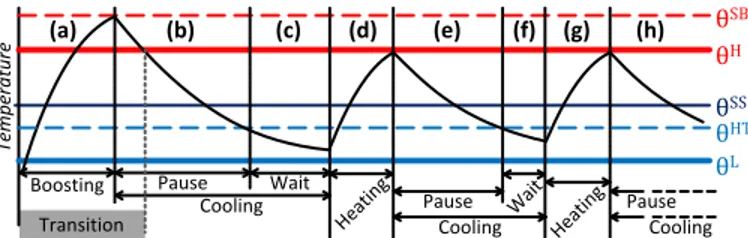
Fig. 4 demonstrates how the transient-based heuristic works, by showing the temperature curve for one of the thermal nodes. The curve starts at the exact moment that the transition to the new map is started. The transition interval ends when all the nodes are in their valid temperature ranges. Since only one of the nodes is shown here, the transition time cannot be observed directly, therefore it is indicated by the gray area at the lower left corner of Fig. 4. Boosting is shown in interval a: the temperature increases beyond 𝜃𝑛𝐻 and continues to 𝜃𝑛𝑆𝐵. This
helps to achieve a shorter transition time, as discussed before. Apart from boosting, other operations during the transition are similar to the operations after the transition.
3) Operations After the Transition
Just after transition, the map is enforced. But since a node’s temperature will naturally decrease the temperature will eventually fall below 𝜃𝑛𝐿 if no or little power is applied to it. Therefore, a heating sequence should be applied at some point, before the temperature falls out of range. This point is marked with a temperature level named Heating Trigger and denoted by 𝜃𝑛𝐻𝑇 for node 𝑛 (𝜃𝑛𝐻𝑇> 𝜃𝑛𝐿). The heating sequence should be
applied when the temperature of node 𝑛 falls below 𝜃𝑛𝐻𝑇. The
difference between 𝜃𝑛𝐻𝑇 and 𝜃𝑛𝐿 provides sufficient time for the
node to wait for gaining access to the TAM without its temperature falling below 𝜃𝑛𝐿. In Fig. 4, the heating is required
at the beginning of the interval c, but since the TAM is not available, the node waits. At the beginning of the interval d the node has finally gained access to the TAM and the heating begins.
Heating should stop when the temperature reaches 𝜃𝑛𝐻. The
time it takes to get back to the low temperature limit could be
Figure 4. Transient-based heuristic demonstrated using a temperature curve.
Te m p er a tu re θSS θSB θHT Transition Pause Wait Cooling Heat ing Pause Cooling θH θL Pause Cooling W ait Heat ing (a) (b) (c) (d) (e) (f) (g) (h) Boosting
utilized to heat up other nodes that need heating. In a situation that a module consists of multiple active thermal nodes, the heating sequence could only be applied if all of these thermal nodes have temperatures lower than their high temperature limit.
4) TAM Access Management
The nodes that simultaneously require heating should be accommodated within the available bandwidth of the TAM. This bandwidth might not be sufficient for all of them and, therefore, the nodes that need heating more than others should be prioritized. The priorities for using the TAM are determined based on the regional need for heating (denoted by 𝑑𝑛 around
a node 𝑛). The value of 𝑑𝑛 is recomputed whenever node 𝑛
needs heating (during offline schedule generation). A node requires heating in the following two situations: (i) When 𝜃𝑛<
𝜃𝑛𝐻𝑇, after the transition, for example the interval c in Fig. 4. (ii)
When 𝜃𝑛< 𝜃𝑛𝑆𝐵, during the transition, for example the interval
a in Fig. 4. In the following, we explain how to calculate 𝑑𝑛 for
the situation i. Regional need for heating for situation ii is obtained in a similar manner by replacing 𝜃𝑛𝐻𝑇 with 𝜃𝑛𝑆𝐵.
Equation 1 is re-written, with the approximate derivatives, as
𝑨×(𝜣𝐻𝑇−𝜣 )
𝑇 + 𝑩 × 𝜣 = 𝑷̅ + 𝑫 × 𝑷
𝐻𝑆. (12)
The input power, 𝑷, in (1) is substituted with the stray power, 𝑷̅, plus the PWM power of heating sequences, 𝑫 × 𝑷𝐻𝑆. Vector
𝑫 is the vector form of the regional need for heating and consists of 𝑑𝑛s. Equation 12 is written for one test cycle with period 𝑇 which is a very short time. The equation is then solved for the nodes that need heating as follows.
𝑑𝑛=
∑𝑁−1𝑘=0𝑎𝑛,𝑘×(𝜃𝑘𝐻𝑇− 𝜃𝑘)
𝑇 + ∑𝑁−1𝑘=0𝑏𝑛,𝑘× 𝜃𝑘− 𝑝̅̅̅𝑛
𝑝𝑛𝐻𝑆
(13) The regional need for heating, 𝑑𝑛, depends on the required
heating for node 𝑛 (consider the summations when 𝑘 is equal to 𝑛), on the required heating that is related to the adjacent nodes (consider the summations when 𝑘 denotes an adjacent node to 𝑛), and on the average power of the corresponding heating sequence, 𝑝𝑛𝐻𝑆. The regional need for heating for a node has the
highest dependency on the node itself, and then a relatively high dependency on the adjacent nodes (this characteristic is captured by the temperature model). The influence of other nodes located far away from the targeted node is small. The heat transfer between nodes is taken into account automatically, since (13) is derived from the temperature equation, (1), and includes the thermal conductances from matrix 𝑩. This is reflected by 𝑏𝑛,𝑘 in (13).
Equation 13 ensures that the priority for using the TAM is given to the regions that need longer heating times, for example because of large (𝜃𝑛𝐻𝑇− 𝜃𝑛) and small 𝑝𝑛𝐻𝑆. Furthermore, the locality of this heuristic is helpful because adjacent nodes are likely to be in the same module and therefore these nodes will receive some desirable heating sequence (𝑝𝑛,𝑘𝐻𝑆) or heat
transferred from module 𝑛. An effect of the interplay between priorities could be seen in Fig. 4. The waiting period in the interval f is much shorter than the waiting period in the interval
c. The length of a waiting period depends on the other nodes’s
priorities in addition to the node 𝑛’s priority.
As discussed before, the performance of the transient-based heuristic strongly depends on the stop boosting, 𝜃𝑛𝑆𝐵, and
heating trigger, 𝜃𝑛𝐻𝑇, temperatures. One example is the
priorities calculated using (13), since they depend on 𝜃𝑛𝐻𝑇 after
the transition and on 𝜃𝑛𝑆𝐵 during the transition. Efficient values
for these temperature levels for each temperature map and each thermal node are found using a Particle Swarm Optimization (PSO) technique. Particle swarm optimization is a well-known iterative population-based optimization metaheuristic. A canonical form of PSO [22] is used in this paper in a straightforward manner.
E. Remarks
The proposed approaches support also heating sequences generated by a Built-In Self-Test (BIST) engine. An example for the use of BIST engines during burn-in in order to achieve high toggle coverage is reported in [10]. Such BIST engines that stimulate high switching activities in a certain area of the IC under burn-in can be used to produce heating sequences online. The only difference, in our context, is that if the BIST engine does not occupy TAM, then it can be scheduled at any time as needed. For instance assuming that module 𝑚𝑘 can receive its
heating sequence from an adjacent BIST engine that is not occupying TAM, the 8th line for the LP formulation in Fig. 2
should be changed to: (∑𝑘−1𝑚=0
𝐷
𝑚+
∑𝑀−1𝑚=𝑘+1𝐷
𝑚)≤ 𝑊
. Thesituation for the transient-based heuristic is even simpler, since the algorithm only needs to know that module 𝑚𝑘 can receive
its heating sequence at any time. Then, 𝑚𝑘 does not need to
compete with others for TAM access. Consequently, there is no need to evaluate the regional need for heating for 𝑚𝑘.
The proposed approaches in section III make it possible to perform burn-in based on heating sequences without requiring a heat chamber. One of the situations when a heat chamber might be required is for the ICs that are designed to work in an extremely high temperature environment. For example, a microcontroller for a car engine is designed with low power in order not to raise too much its temperature from the very high ambient temperature in the engine area. When such a chip is tested or operates with regular low ambient temperature, it is impossible to have enough power density to boost its temperature to its usual high level in normal working condition. Another such situation is when some parts of an IC (e.g., package pins, die to pin connections, and the interposer) cannot be heated up sufficiently by input stimuli. In such cases, an extremely hot burn-in condition might be required that is not achievable by exclusive use of heating sequences. Even in such cases the use of the methods proposed in this paper for enforcing the temperature gradients will still be useful. The proposed algorithms do not need any modifications to work under such situations, except to set a large ambient temperature corresponding to the heat chamber temperature.
The proposed transient-based heuristic allows the IC to be divided into a desired number of thermal nodes, 𝑁. A large 𝑁 means high resolution and translates into higher computational effort. Therefore, the resolution can be restricted if the available computational power is limited.
In this paper, as mentioned previously, it is assumed that the temperature maps capable of identifying the gradient-dependent defects are given. Furthermore, it is assumed that the combination of the given tests and heating sequences (mixed with cooling intervals) is capable of enforcing the desired
temperatures on the specified modules.
IV. TEMPERATURE-GRADIENT BASED TEST
For the temperature-gradient based test, the goal is to make sure that the tests are performed when the temperature gradients are enforced. This means that the specified temperature maps should be enforced before the test and then maintained during the test. The straightforward algorithm and the fast heuristic, which are proposed in the following, do this differently.
A. Straightforward Algorithm
This algorithm works by changing between two modes, the
temperature construction mode and the test mode. Initially the
temperature construction mode is activated and it enforces the specified temperature map using a method similar to the transient-based heuristic proposed in section III.D. Then the test mode is activated and the tests that are scheduled with a third party algorithm (e.g., scheduling method proposed in [24]) are applied. The test temperatures are simulated at design time and as soon as at least one of the thermal nodes is out of its specified range, the test mode is paused and the temperature construction mode takes over again. When all thermal nodes are brought into the specified temperature ranges, the temperature construction mode is paused and testing resumes.
Similar to the transient-based heuristic, if the temperature of a node is lower than the heating trigger temperature, it should be heated by applying the heating sequence to it. If there are many nodes that need heating (more than what the TAM can support), priority is given to those with higher regional need for heating as defined in section III.D. The construction mode, unlike the transient-based heuristic, should not heat the nodes up to their high temperature limit since the power of the tests that are applied immediately after the construction mode may rapidly heat up the node beyond high temperature limit. Therefore, Testing Trigger temperatures which are denoted by 𝜃𝑛𝑇𝑇 for node 𝑛 (𝜃𝑛𝐻𝑇< 𝜃𝑛𝑇𝑇< 𝜃𝑛𝐻) are introduced here. During
the temperature construction mode, the heating for node 𝑛 stops as soon as the temperature reaches 𝜃𝑛𝑇𝑇.
In the test mode, as soon as the temperature of a node reaches the high temperature limit, the test mode is immediately paused, the temperature construction mode is activated and, consequently, a cooling interval is applied. The cooling continues until the node is cooled down to the testing trigger temperature, 𝜃𝑛𝑇𝑇, and then the node is ready for testing again.
The actual activation of the test mode will also depend on the temperatures of the other nodes. Efficient values for testing trigger temperatures, 𝜃𝑛𝑇𝑇, for each map are found using a particle swarm optimization technique along with 𝜃𝑛𝑆𝐵 and 𝜃𝑛𝐻𝑇.
The inputs to the methods proposed here include the inputs to the methods proposed in section III as well as the test specifications (e.g., test switching activities). The output is a set of offline schedules, generated based on temperature simulations. There is no need for temperature sensors and the precision of the achieved temperature maps depends on the temperature model. Although, generating such offline schedules is the focus of this paper, the proper values for the heating trigger, 𝜃𝑛𝐻𝑇, stop boosting temperatures, 𝜃𝑛𝑆𝐵, and
testing trigger temperatures, 𝜃𝑛𝑇𝑇, which result in a rapid test, could also be considered as the outputs that provide a basis for an online scheduling scenario. In this case, temperature sensors are used and the precision depends on the temperature sensors.
Such online approaches are however beyond the scope of this paper.
The straightforward algorithm is simple, and allows the choice of a desired arbitrary test schedule that is used in the test mode. But the overall test application time offered by this method is very long. Note that the total test application time also includes times spent for temperature construction.
B. Fast Heuristic
The fast heuristic schedules the tests together with the heating sequences such that the specified temperature map is maintained. This way, a shorter test application time can be achieved. An illustrative example for the proposed method is given in Fig. 5 for a single thermal node. The proposed technique has similarities to the temperature construction algorithm in the previous section. For example, stop boosting temperature, 𝜃𝑛𝑆𝐵, indicates that the boosting should stop, as illustrated at the end of interval a in Fig. 5. After being too warm, the node should cool until its temperature gets below the testing trigger temperature, 𝜃𝑛𝑇𝑇, as shown in interval b.
When the temperatures for all of the other thermal nodes covered by module 𝑚 are between their high temperature limit, 𝜃𝑛𝐻, and their heating trigger, 𝜃𝑛𝐻𝑇 (𝜃𝑛𝐻> 𝜃𝑛𝐻𝑇), testing may
start, as in interval c in Fig. 5. All other nodes should be within their temperature limits [𝜃𝑛𝐿 𝜃𝑛𝐻]. Testing continues until the
temperature of at least one of the nodes goes beyond the high temperature limit 𝜃𝑛𝐻 or falls below the heating trigger 𝜃𝑛𝐻𝑇. For
example at the end of interval c, the node is too cold for testing and a heating interval should be introduced. Note that the TAM may no longer be available and therefore the node is waiting for access to TAM in interval d.
Finally, when access to the TAM is obtained, the heating sequence is applied in interval e. In order to start heating, all nodes covered by a module should be colder than the high temperature limit since the heating sequence for one node is very likely to inject power to other nodes in the same module (as explained in section III.D). Heating continues until the temperature goes beyond the testing trigger temperature and, then, the test resumes as in interval f in Fig. 5. When the temperature reaches the high temperature limit, a cooling interval is introduced as in interval g. This procedure continues until all tests corresponding to the current temperature map are completed.
As mentioned before, nodes will compete for access to the TAM and, therefore, some of them should be prioritized. First the nodes that require heating (not the tests) are granted access to TAM. This helps to keep the temperatures most of the time within the specified limits and, thus, keep the flow of the tests uninterrupted. Note that if only one node falls out of its specified range, all tests must be interrupted until the map is achieved again. This will waste a lot of time, since the tests for the modules that are in their specified range should also be interrupted. The priorities for the nodes that require heating is
Figure 5. Fast heuristic demonstrated using a temperature curve.
θTT θSB
θHT
Boost Test Heat
θH
θL
Wait Test Cool Test
(a) (b) (c) (d) (e) (f) (g) (h)
determined based on the regional need for heating as proposed in section III.D.
If the TAM has left with some available bandwidth after the heating sequences are scheduled, the modules that are thermally
qualified may resume their tests. A module is thermally qualified if none of the nodes that correspond to that module are
demanded by the previously discussed rules to receive heating, wait for heating, or receive cooling. The priority is given to the modules that are expected to offer long test endurance. The test endurance is denoted by 𝑒𝑚 for module 𝑚, and is defined as
𝑒𝑚= 𝑡𝑡𝑚× 𝑟𝑚 . (14)
The test endurance is directly proportional with the
remaining test size denoted by 𝑟𝑚 for module 𝑚. The larger the
remaining test size, the longer the test endurance. The thermal
tolerance, denoted by 𝑡𝑡𝑚 for module 𝑚, is the other
contributor to the test endurance. High thermal tolerance, 𝑡𝑡𝑚,
indicates that the module is capable of receiving tests for a relatively long time without exceeding the specified thermal limits. Therefore, a module with large thermal tolerance may remain under test for a relatively long time. The thermal tolerance is defined as
𝑡𝑡𝑚= min𝑘 {∆𝑘} . (15) In (15), it is assumed that module 𝑚 covers 𝐾 active thermal nodes. ∆𝑘 (𝑘 = 0, 1, … , 𝐾 − 1) denotes the expected thermal distance to a temperature limit for node 𝑘 and is defined as
∆𝑘= {𝜃𝑘 𝐻− 𝜃
𝑘 , 𝑖𝑓 𝑢𝑝𝑐𝑜𝑚𝑖𝑛𝑔_𝑡𝑒𝑠𝑡𝑠_𝑝𝑜𝑤𝑒𝑟 > 𝑝𝑘𝑆𝑆
𝜃𝑘− 𝜃𝑘𝐻𝑇 , 𝑖𝑓 𝑢𝑝𝑐𝑜𝑚𝑖𝑛𝑔_𝑡𝑒𝑠𝑡𝑠_𝑝𝑜𝑤𝑒𝑟 ≤ 𝑝𝑘𝑆𝑆
(16) As mentioned in section III.B, the desired steady state power 𝑝𝑘𝑆𝑆 is the power that results in a temperature equal to 𝜃𝑛𝑆𝑆=12×
(𝜃𝑛𝐿+ 𝜃𝑛𝐻). Equation 16 indicates that if the upcoming tests
have relatively high average power, then it is likely that the thermal node exceeds the high temperature limit and, therefore, the difference between the current temperature, 𝜃𝑘, and the high
temperature limit, 𝜃𝑘𝐻, is a good measure for thermal tolerance.
Similarly, for a relatively low power test, it is more likely that the temperature falls below the heating trigger in the future. Therefore, the difference between the current temperature, 𝜃𝑘,
and the heating trigger temperature, 𝜃𝑘𝐻𝑇, is a good measure for
thermal tolerance. Thermal tolerance, 𝑡𝑡𝑚, is defined as the
smallest ∆𝑘 (𝑘 = 0, 1, … , 𝐾 − 1) since as soon as a single node
is out of the specified range [𝜃𝑛𝐿 𝜃𝑛𝐻], disregarding of the temperatures of the other nodes, test should be interrupted. Note that if the temperature falls below 𝜃𝑛𝐻𝑇, only for a node in module 𝑚, then the test is interrupted only for module 𝑚.
A proper value for the testing trigger temperature, 𝜃𝑛𝑇𝑇 is selected so that the temperature variation during test (caused by the variations in the test power) rarely results in the temperatures below 𝜃𝑛𝐻𝑇or above 𝜃𝑛𝐻. Every time that 𝜃𝑛𝐻𝑇or 𝜃𝑛𝐻
are violated, the test must be interrupted and a heating or cooling interval must be introduced, respectively. Since these are time consuming, a proper 𝜃𝑛𝑇𝑇 value helps to obtain a short
test application time by reducing the number of interruptions. Besides the testing trigger temperature, stop boosting and heating trigger temperatures (𝜃𝑛𝑆𝐵 and 𝜃𝑛𝐻𝑇 respectively) have a
considerable effect on the test application time and therefor proper values for them should be found. A particle swarm optimization technique is used to find the proper values for 𝜃𝑛𝑆𝐵,
𝜃𝑛𝐻𝑇, and 𝜃𝑛𝑇𝑇 for each map. Similar to the previous sections, the
canonical PSO [22] is utilized in a straightforward manner. V. TEMPERATURE MAP ORDERING TECHNIQUE
The order in which the maps are enforced has a considerable impact on the overall burn-in and test time. Since there are usually a number of temperature maps to be applied, their ordering is important. In this section we present methods to rapidly obtain a proper order for temperature maps that results in a short burn-in and test time.
To simplify the discussions, let us assume that the temperature map for a thermal node is represented by the middle value of the specified temperature range 𝜃𝑛𝑆𝑆=12×
(𝜃𝑛𝐿+ 𝜃𝑛𝐻). As an example, assume that an IC has two thermal
nodes and the initial temperature is 30℃. The temperatures specified in map 𝜇0 are denoted by {𝜃0𝑆𝑆, 𝜃1𝑆𝑆}2. This means that
temperatures 𝜃0𝑆𝑆 and 𝜃1𝑆𝑆 are specified by map 𝜇0 for nodes 0
and 1, respectively. Assume that there are three temperature maps denoted by 𝜇0, 𝜇1, and 𝜇2. These maps specify the
following temperatures: 𝜇0 = {110℃, 90℃}, 𝜇1 = {40℃, 50℃}, and 𝜇2 = {110℃, 80℃}, respectively. These
temperature maps are represented in Fig. 6 by three points in a Cartesian space. The temperature for node 0 is represented by the horizontal axes, 𝜃0, and for node 1 by the vertical axes, 𝜃1.
The initial order of temperature maps {𝜇0, 𝜇1, 𝜇2} requires a
long time to increase the temperature for node 0 from 30 to 110 (𝑎0 in Fig. 6a), then decrease it to 40 (𝑎1 in Fig. 6a), and then
again increase it from 40 to 110 (𝑎2 in Fig. 6a). This process
will take a long time due to the required large temperature changes. In contrast, it is much faster to work with the maps ordered as {𝜇1, 𝜇2, 𝜇0}, since in this case, the required
temperature changes consist of smaller temperature variations, as shown in Fig. 6b.
As discussed earlier, in order to minimize the overall transition time for burn in, a particle swarm optimization finds the proper values for stop boosting and heating trigger temperatures (𝜃𝑛𝑆𝐵s and 𝜃𝑛𝐻𝑇s, respectively). The map orders
should be optimized along with these temperatures, since all of these factors have a crucial effect on the overall transition time for a given set of temperature maps. The naïve approach to find proper map orders is to introduce them as decision variables into the PSO along with 𝜃𝑛𝑆𝐵s and 𝜃𝑛𝐻𝑇s. Experiments showed that this naïve approach takes very long CPU time to complete. Since the optimized values for 𝜃𝑛𝑆𝐵 and 𝜃𝑛𝐻𝑇 depend on the map
order, different map orders results in different optimized values for 𝜃𝑛𝑆𝐵 and 𝜃𝑛𝐻𝑇.
The initial PSO population in the naïve approach consists only of random solutions (random 𝜃𝑛𝑆𝐵s, 𝜃𝑛𝐻𝑇s, and random map
orders). Introducing a relatively good map order into the initial population of PSO (among other initial solutions that are random) will help to speed up the search. This approach is denoted by A1. The idea for approach A1 is to rapidly find a potentially good map order using some initialization heuristic and introduce it into the initial PSO population. By doing this, the search should speed up while the quality of the final values for 𝜃𝑛𝑆𝐵s and 𝜃𝑛𝐻𝑇s are kept reasonably high. In the majority of
cases, PSO finds a better map order than the one produced by 2 The notation {𝑎
0, 𝑎1, …, 𝑎𝐾} is used to represent an ordered sequence of