Is it possible to avoid bad impacts by using good fuel ethanol?

(1)

bad impacts by using

good fuel ethanol?

report 6331 • february 2010

(2)

Authors:

Göran Berndes and David Bryngelsson

Chalmers University of Technology, Gothenburg, Sweden Gerd Sparovek,

University of Sao Paulo/ESALQ, Piracicaba, SP, Brazil

SWEDISH ENVIRONMENTAL PROTECTION AGENCY

(3)

Orders

Phone: + 46 (0)8-505 933 40 Fax: + 46 (0)8-505 933 99

E-mail: natur@cm.se

Address: CM Gruppen AB, Box 110 93, SE-161 11 Bromma, Sweden Internet: www.naturvardsverket.se/bokhandeln

The Swedish Environmental Protection Agency Phone: + 46 (0)8-698 10 00, Fax: + 46 (0)8-20 29 25

E-mail: registrator@naturvardsverket.se

Address: Naturvårdsverket, SE-106 48 Stockholm, Sweden Internet: www.naturvardsverket.se

ISBN 978-91-620-6331-3.pdf ISSN 0282-7298 © Naturvårdsverket 2010

Digital Publication

(4)

(5)

Preface

Much of the global production of biofuels is considered to be non-sustainable. Brazilian sugarcane ethanol, on the other hand, is normally judged to be “good”. Swedes are anxious only to use fuel ethanol with the best climate characteristics in a life-cycle perspective, and the bulk of ethanol used in Sweden comes from Brazil.

The Swedish Environmental Protection Agency has identified some crucial issues which often are left out from discussions. These might be of extra importance for the Swedish ethanol use:

- Might Swedish demand for good ethanol indirectly raise the demand for “bad” ethanol, such as US maize ethanol with fossil energy input? Or is it possible to encourage the production of exclusively “good” ethanol by choosing such (certi-fied) ethanol? This depends on how the international market for fuel ethanol works.

- To what extent does increased Swedish, or European, demand encourage the long-term supply of ethanol? What supply elasticities are there in Brazil and glob-ally? If increased European use only means that we take hold of a fixed supply, the climate benefit compared to fossil fuels will not occur.

The analyses are further complicated by the fact that there might be land-use com-petition between fuel, feedstuffs and food. When available land becomes more limited, increased production might necessitate breaking new soil, which could lead to emissions of climate-changing gases elsewhere. Consequently it is not only the fuel market itself that needs to be analysed.

The Swedish Environmental Protection Agency asked the Chalmers University of Technology in Gothenburg, Sweden to study these issues in a comprehensive con-text. Chalmers jointly performed the study with researchers in Sao Paulo, Brazil. Authors are Göran Berndes and David Bryngelsson at Chalmers and Gerd

Sparovek at University of Sao Paulo/ESALQ. The authors alone are responsible for the contents of the report, which should not be regarded as necessarily reflecting the views of the Swedish Environmental Protection Agency. The contact at the Swedish EPA was Mats Björsell.

(6)

1 Introduction

Sweden is anxious to use only “good” fuel ethanol with the best climate perform-ance in a life cycle perspective. A large part of the ethanol used in Sweden has been imported from Brazil, and Brazilian ethanol is considered to have good such qualities. Also, Swedish cereal ethanol has a good climate performance compared to the average for cereal ethanol, thanks to favourable process integration and location leading to low Greenhouse gas (GHG) emissions from the conversion process (Börjesson 2008).

However, depending on how the international ethanol and food market functions Swedish consumption of good ethanol may lead to undesirable so-called indirect effects. For example, if the USA is the marginal producer on the world ethanol market; an increased Swedish import demand may indirectly induce increased maize ethanol production in the USA (with a lower mitigation benefit than Brazil-ian ethanol), despite that the ethanol imports to Sweden comes from Brazil. Simi-larly, if more Swedish cereals are channelled to Swedish ethanol plants the vol-umes lost for the food sector need to be produced somewhere. If this additional production is achieved based on expanding cropland into forests (or by cultivating grassland with high soil carbon content) the resulting GHG emissions can be higher than what is gained from increased Swedish cereal ethanol production.

Thus, how the international market for cereals and for fuel ethanol looks like is of vital importance for the possibilities to conclude whether the marginal net climate benefit of expanding the use of domestic and Brazilian ethanol is favourable1_.

This report primarily focuses on the case of Brazilian ethanol, which is the major source of the Swedish ethanol imports. To assess the GHG emission impact from Swedish/European use of Brazilian ethanol one needs to understand the properties of ethanol markets. The implications might be, at the extreme, that when undertak-ing life cycle assessments it would be relevant to use global average ethanol LCA-data or LCA-LCA-data representative for the marginal supplier to the world market, instead of LCA-data for the sugarcane ethanol actually used.

The report contains a description of the international ethanol fuel supply character-istics. The description is given for the present situation but also includes a discus-sion of possible developments using 2020 as time horizon. Based on this descrip-tion the report discusses possible effects of Swedish ethanol use and specifically our import and use of Brazilian ethanol.

1

It is also crucial to come further in the discussion about responsibility of individual biofuel producers for indirect emissions taking place – one alternative could be to place the responsibility on those that actually cause the emissions. However, this discussion goes beyond the scope of this report

(9)

Besides climate performance, many other environmental and socio-economic as-pects have been raised as concerns related to biofuels, including Brazilian ethanol. Therefore, we also present results from investigations of the socioeconomic and environmental effects of the ethanol expansion in Brazil 1996-2006, with a view on future development. Linked to this, we outline an alternative expansion model that might mitigate some of the risks and negative effects connected to conventional ethanol production in Brazil and we discuss prospects for implementation of such an expansion model within a certified market.

We also discuss the possibilities for Sweden – being a country with relatively small transport fuel use compared to many other countries – to influence the Brazilian ethanol production at large by linking specific requirements on how the ethanol that Sweden imports should be produced. This discussion is based on ongoing studies, including stakeholder interviews.

The work has been guided by a number of lead questions, including:

• Could we choose to stimulate production of exclusively 100% “good” ethanol, when we buy such (certified or not) good ethanol?

• To what extent do we have an international global market, what elements of “world market” is there today?

• To what extent does an increased European demand stimulate supply? What are supply-elasticities in Brazil and globally?

• Is the supply curve vertical? If so, an European increased use means that we “lay hands on” the fixed supply, so that climate advantage does not occur.

• How are expanding production capacities in Brazil (and other parts of the world) influenced when Europe very quickly raises the demand for etha-nol?

• How is production in Brazil (and other parts of the world) influenced by demand for certified “good” ethanol? Is there evidence that production for niche markets can influence the conventional production, and if so, how?

The report was commissioned by the Swedish Environmental Protection Agency and has been produced jointly by the authors, using also support from IEA Bio-energy Task 30 and the Swedish Energy Agency. The report is partly based on earlier and ongoing research and the authors want to acknowledge important con-tributions to this research from Andrea Egeskog at Dept. of Energy and Environ-ment, Chalmers University of Technology, Sweden; Flavio Luiz Mazzaro de Freitas and Alberto Barretto at ESALQ, Sao Paulo University, Brazil; Sergio Martins and Rodrigo Maule at Entropix Engineering, Piracicaba, Brazil; Stina Gustafsson, formerly at Chalmers and now at the Swedish Environmental protec-tion Agency; and Anders Åhlén, formerly at Chalmers and now at McKinsey, Stockholm, Sweden.

(10)

Mats Björsell and Nanna Wikholm at the Swedish Environmental Protection Agency have supported the writing by reviewing and providing constructive feed-back on draft reports.

(11)

2 The present situation for

ethanol and bioenergy in

general

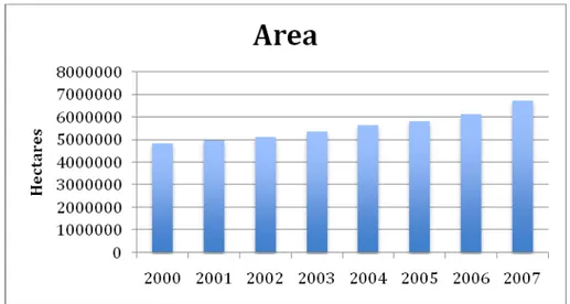
Today, biomass (mainly wood) contributes some 10% to the world primary energy mix, and is still by far the most widely used renewable energy source (Figure 2.1). While bioenergy represents a mere 3% of primary energy in industrialized countries, it accounts for 22% of the energy mix in developing countries, where it contributes largely to domestic heating and cooking, mostly in simple inefficient stoves.

Figure 2.1. Share of bioenergy in the world primary energy mix. Source: based on IEA (2006) and IPCC (2007).

Over the last three decades, issues of energy security, increasing prices of fossil fuels and global warming have triggered a renewed interest in biomass for the pro-duction of heat, electricity and transport fuels, with many countries introducing policies to support bioenergy, also as a means of diversifying the agricultural sec-tor. This has been accompanied by significant developments in conversion proc-esses, with cleaner more efficient technologies being introduced into the market and several others at the research, development and demonstration stage. The bio-mass resource base is potentially large, and so are the opportunities for its in-creased use in different energy segments in industrialized and developing coun-tries.

The bioenergy sector has witnessed significant growth in recent years, in particular in relation to biofuels for the road transport sector, which has grown considerably faster than the heat and electricity sectors. While the development of the bioenergy industry remains very dependent on regional policies, this industry is at the same time becoming increasingly globalised as a result of an emerging global trade in biomass products such as pellets and ethanol. The biofuel market is globally

(12)

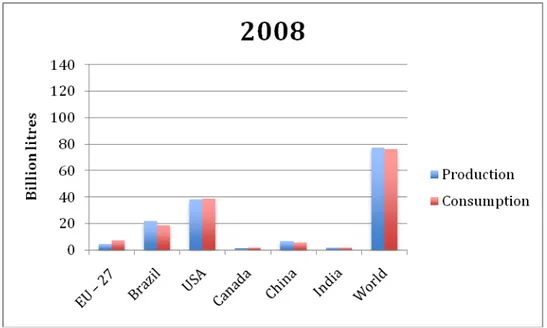
dominated by ethanol, but in the EU biodiesel makes up a larger share. 54% of EU-27s production of biodiesel takes place in Germany and has been driven by a total exemption from fuel taxes (Birur, Hertel and Tyner 2007). The German tax exemp-tion has recently been replaced by quotas. The producexemp-tion and consumpexemp-tion of ethanol is dominated by a few countries with the USA and Brazil in the lead (Figure 2.2).

The relative importance of drivers for consumption and production of ethanol vary between countries, since they place different emphasis on the underlying objectives – with the most common being energy security, climate change mitigation, and revitalization of the national agricultural sector (FAO 2008) (M. Banse, et al. 2007). Emphasis on such diverse objectives results in a wide variety of policy driven incentives for both production and consumption of ethanol.

Figure 2.2: Ethanol production and consumption by region during 2008. Source: OECD-FAO Agricultural Outlook Database.

(13)

3 Will increased ethanol use in

Sweden lead to increased

ethanol production in Brazil?

3.1 Aspects influencing the impacts of

Swedish ethanol use

Many aspects influence the impacts of Swedish ethanol use – not the least the shap-ing of policies and regulatshap-ing mechanisms – and it is far from straightforward to project the effects of Swedish ethanol use on international ethanol production and trade. Below, aspects judged as important are briefly accounted for with the aim to provide a basis for proposing features of the international response to increased Swedish ethanol use.

3.1.1 Ethanol consumption and price elasticities

Varying rationales for countries promoting biofuels such as ethanol have resulted in a wide variety of policy driven incentives for both production and consumption of ethanol. The global ethanol market is thus very complicated and heavily dis-torted due to various market interventions such as fixed mandates, production tar-gets, import tariffs and subsidies. According to FAO, direct support to production and consumption has the largest distorting effects, while research support is the least distorting (FAO 2008).

Birur, Hertel, & Tyner (2007) calculated price elasticities of substitution between ethanol and oil, based on historical data from 2001 to 2006, and came up with 3.0 for the USA, 2.75 for the EU and 1.0 for Brazil. The price elasticity of demand can be very elastic in areas where ethanol is just competitive with oil and the technical limits are not yet reached (M. Banse, et al., 2008b). These technical limits depend significantly on the infrastructure in the region and the vehicle pool used.

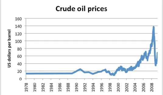
One should be aware though, that these elasticities have been calculated based on data during a period of great change, where consumption of fuel ethanol in most places has started from almost zero. There were also other forces at play on the European and American markets that may not have had so much to do with price elasticity of demand. The oil price has been constantly increasing since 2001 until it peaked in mid 2008 and then decreased sharply to a bottom level in December the same year (Figure 3.1). At the same time there have been a number of political decisions regarding ethanol for energy security, climate change mitigation etc, mandating certain blends of ethanol in petrol. The consumption of ethanol has hence increased at a time when the ethanol price has moved in favour of oil, but the correlation cannot be fully explained by economic theory of price links.

(14)

The situation is fundamentally different for Brazil, however, which is the only mature market for fuel ethanol (M. Banse, et al., 2008b) with a long history of policy support, which has now been phased out. A large share of the car-fleet in Brazil is full flexibility vehicles (FFV) and the consumers can therefore at every re-fuelling choose to buy the cheapest fuel blend. This can explain Brazil’s unity elasticity. The rapid decrease in ethanol consumption in Sweden following the oil price decrease in the end of 2008 is another illustrative example of close connec-tions between oil prices and ethanol consumption in countries having a substantial share of ethanol consumption connected to flex fuel vehicles (E85 in the case of Sweden). In countries where the major part of the ethanol volumes are used in low level gasoline blends, it is the gasoline producers rather than the fuel consumers that define the price elasticity of substitution between ethanol and oil. The way policies are formulated influence elasticities. Strict biofuel obligations, e.g. requir-ing a minimum level of blendrequir-ing in gasoline and diesel, results in inelastic demand while financial incentives such as tax exemptions at the pump leads to more elastic demand.

Since the feedstocks presently used for ethanol production have alternative use in the food sector, ethanol prices can also be influenced by the food sector develop-ment that influences the feedstock costs. This influence of course also goes in the opposite direction. Demand for ethanol has for instance created a floor price for sugar and when oil prices are high enough to make sugarcane ethanol competitive on the energy market sugar prices develop along the same pattern as oil prices.

Figure 3.1: Development of oil prices over time. Peaking in July 2008 the oil price decreased sharply to a bottom price well below US$40 per barrel in December the same year. Increasing since then the crude oil price was around US$50 per barrel in April 2009. Source: EIA (2009).

(15)

3.1.2 Ethanol production costs in different countries/regions

The cost of production varies substantially between different areas and production systems. Figure 3.2 presents indicative production costs of ethanol and biodiesel from different crops and from animal fat in the main production regions in 2007. It is important to keep in mind that biofuel production costs are calculated for spe-cific production and conversion contexts, which vary over time and space. The production costs are sensitive to feedstock costs as well as capital costs, and devel-opment towards larger plants – which has been the trend; the capacity of new plants is as a rule above 200 million litre per year – reduces total production cost2. The level of co-product revenues is another important factor.

Figure 3.2. Indicative production costs of ethanol and biodiesel from different crops and from animal fat in the main producing regions in 2007. Source: E4tech (2008).

For instance, Goldemberg (2007) reports that Brazilian sugarcane ethanol produc-tion costs can be as low as US$0.2 per litre and, similarly, lower producproduc-tion costs than given in Figure 3.2 can be calculated for cereal or beet ethanol if lower feed-stock/capital costs and/or higher co-product revenues are used. CFC (2007) report ethanol production costs ranging from about US$ 0.40 – 0.50 per litre for maize

2

Feedstock costs account for approximately half of the cost of sugarcane ethanol production, and a greater share of costs in the case of the other first generation ethanol production pathways, such as corn ethanol.

(16)

ethanol in the USA to US$ 0.50 – 0.80 per litre for European ethanol produced from wheat or sugar beet.

Nevertheless, looking at the ethanol production from a cost effectiveness perspec-tive, the choice of feedstock would be sugarcane and the country of production would be Brazil, which has the lowest production costs and also potential as well as near term capacity to expand the ethanol production substantially. The Brazilian ethanol becomes cost competitive against oil at a crude oil price of about US$35-45/bbl (Banse, et al., 2008a) (BNDES; CGEE; 2008), while the oil price needs to be roughly twice as high for the US maize ethanol and up to three times higher for European ethanol to compete with oil3_.

From a purely economic perspective, Brazil should supply the market until the marginal cost of expansion in Brazil reaches that of another region, e.g. ethanol based on cassava from Thailand, which becomes cost competitive at an oil price of US$ 45/bbl (Schmidhuber 2007). Production in the USA or EU would not begin until all cheaper options were exhausted and marginal expansion could be done at the lowest cost in these regions.

However, in addition to the market price of oil the competitiveness of ethanol on the market crucially depends on which policy instruments are in place. The present ethanol production in “high cost” regions such as EU and USA exists due to gov-ernments introducing trade barriers and market distortions, motivated by other than purely economic considerations. Taking USA as an example, existing mandates and trade barriers induce a continued increase in domestic production of maize based ethanol despite that it is much more costly than ethanol from possible import sources (Birur, Hertel and Tyner 2007). Several other countries/regions (e.g., EU, Canada, Australia and China) have also set targets for renewable fuels in the trans-portation sector and many of them also have trade barriers.

3.1.3 Capacity expansion rate constraints

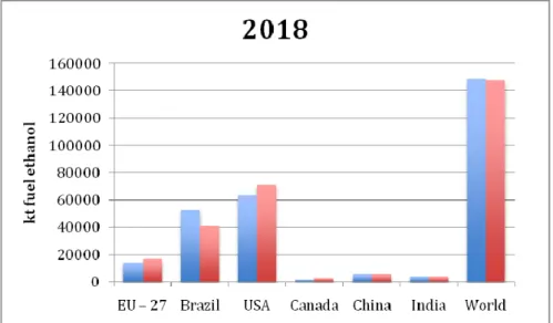
A comparison of Figure 2.2 with Figure 3.3 gives an indication of the expected development of ethanol production and consumption in some major ethanol mar-kets during the period up to 2017. As can be seen, Brazil is expected to expand its ethanol production substantially and despite USA producing more ethanol, Brazil is expected to further establish its position as the main ethanol exporter on the world market. The projected ethanol production in Brazil up to 2018 – according to

OECD-FAO Agricultural Outlook 2009 - 2018 (OECD-FAO 2009) – is shown in

Figure 3.4, depicting a steady increase during the whole period.

3

Also, as will be discussed further below, the oil price influences the production costs for especially the presently available biofuels where feedstock costs make up a major part of the total biofuel cost: higher oil prices means higher costs for diesel, nitrogen fertilizers (since natural gas prices follow oil prices) and other inputs required for the feedstock production.

(17)

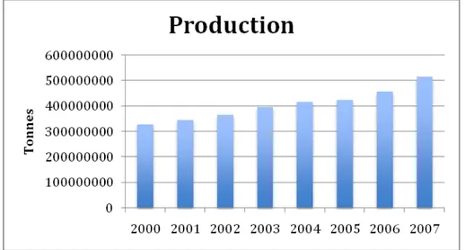
The planned expansion of the Brazilian ethanol production for the coming decade (further discussed later in this report) implies that Brazil plans for meeting both the expected increase in domestic ethanol demand and a significant part of the future international ethanol demand based on substantially increasing its own ethanol production. The development in sugarcane production since year 2000 is shown in Figure 3.5 – Figure 3.7. A comparison of the growth in sugarcane production shown in Figure 3.5 with the projected ethanol production increase up to 2018 shown in Figure 3.4 reveals that the historic and projected future growth rates are similar.

Figure 3.3. Ethanol production and consumption by region for 2017. Source: OECD-FAO Agricul-tural Outlook Database (OECD-FAO 2009).

Figure 3.4: Estimated production of fuel-ethanol from sugarcane in Brazil for 2008 to 2018. Source: OECD-FAO Agricultural Outlook Database (OECD-FAO 2009).

(18)

While short periods of high demand (and prices) for agricultural commodities mainly induces an extended cultivation, longer periods of steady growth of ethanol production, in response to anticipated demand growth, will likely be characterized by both increases in cultivation area and increases in yields through agronomic development, including plant breeding. As agronomic advancements leading to higher sugarcane yields, technology development leading to increased ethanol conversion efficiency at the ethanol plant reduces the area expansion requirement for a given increase in ethanol demand by contributing to improving the ethanol output per hectare. The ethanol conversion efficiency has increased about 3.8% per year during the period 1975 to 2004 (ESMAP 2005).

Based on that the projected expansion rate for Brazilian ethanol is not dramatically different from historic expansion rates it can be considered likely that the increased ethanol production will be accomplished by both increasing agricultural output (extended and intensified sugarcane production) and increasing conversion effi-ciency at the ethanol plants – possibly by introducing technologies for converting part of the cellulosic residue bagasse into ethanol. To the extent that increased ethanol supply will be based on expansion of the sugarcane area experience from the recent period of sugarcane expansion (Sparovek, et al. 2009) as well as studies including Brazilian scenarios for future sugarcane expansion (Zuurbier and van de Vooren 2008) indicate that sugarcane will mainly replace agricultural land in estab-lished agricultural regions and cause little direct deforestation. A large part can be expected to become established on pastures used for extensive cattle production. Productivity increases – especially in pasture production – is projected to mitigate the land expansion pressure arising from sugarcane replacing other agricultural land use, but this can lead to other undesired indirect effects such as increased cattle feed demand leading to higher deforestation pressure of soybean in the Amazon and other preserved biomes (further discussed below).

If demand in some countries/regions grows significantly faster than projected or the production in some other countries/regions grows much slower – the expansion of production capacity in Brazil may reach higher rates, stimulated by high ethanol demand and high prices. However, there are lead times for capacity addition and the maximum rate of capacity addition during the coming decade or so is limited by the number of environmental permits that have been granted to different inves-tors. Thus, even though Brazil has the potential to supply a large share of the global demand for ethanol, the country cannot expand the production at an unlimited pace. With the current economic crisis and relatively low oil prices this upper limit is unlikely to be reached by market forces alone. During phases of high demand-driven growth in ethanol production (e.g. during the peaking oil prices in 2008), capacity expansion restrictions can limit the supply and drive up ethanol prices. Higher prices call for expansion of production in other regions with higher mar-ginal production costs than Brazil. The demand for fuel ethanol is currently

(19)

(spring 2009) much lower than at the peak in 2008 and production expansion is instead limited by reduced profitability4_.

EU and USA have relatively high ethanol production costs and production cost considerations point to mainly other tropical countries as marginal ethanol suppli-ers after Brazil. However, as already mentioned, in addition to the market price of oil, the competitiveness of ethanol on the market crucially depends on which policy instruments are in place. Various market disrupting instruments may lead to etha-nol production still taking place in high cost countries.

Another factor in favour of increased ethanol production in high-cost countries is the uncertain investment climate in some tropical countries identified as promising from the perspective of biophysical potential and production cost. For instance, several countries in Sub-Saharan Africa have large biophysical production poten-tials and there is presently much interest among various international companies and investors. At the same time, lack of knowledge and infrastructure and also limited domestic institutional capacity to support a sound near term large-scale establishment, can make production capacity growth slow in this region5_.

Figure 3.5: Production of sugarcane in Brazil from 2000 to 2007 in tonnes. (FAOSTAT u.d.)

4

www.cepea.esalq.usp.br/english/ 5

Slow growth may also be a prerequisite for avoiding negative socioeconomic and environmental impacts in tropical countries that lack capacity to guide the development according to carefully developed guidelines.

(20)

Figure 3.6. The area under sugarcane cultivation in Brazil. (FAOSTAT u.d.)

Figure 3.7: Expansion of area for sugarcane cultivation in Brazil. (FAOSTAT u.d.)

3.1.4 Land-use dynamics in Brazil

Brazil is a land rich country with vast areas of suitable soils, regular rainfalls and strong insulation. The land is only partly exploited and the production on this land is very dynamic with constant expansion, intensification and changes in crops and in production systems.

Some qualitative patterns have been more or less the same since the colonization; e.g. that land prices are linked to the proximity to urban centres and infrastructure and these prices strongly influence the type of crops or other land-use in each area. The agricultural frontier, which makes up the border between the untouched natural land and the already claimed land, is typically situated far away from any urban

(21)

centres and the infrastructure is poor and sparse. The main use of such land takes the form of low-intensity systems like cattle ranching based on grazing with very low input and low output.

As urban centres emerge and infrastructure improves, land prices go up and exten-sive cattle production gets displaced by high-input-high-output land-uses like crop production, e.g. soybeans or orange trees, and the agricultural frontier with cattle production shifts further into the previously untouched land (Sparovek, et al. 2007).

In some areas also this crop production gets displaced by other land-uses with even higher profits, sugarcane production being a prominent example. This displacement is part of an important interaction between different types of land-uses in Brazil and no crop's environmental impact can be correctly evaluated without considering such inter-land-use interactions (Sparovek, et al. 2007).

The majority of the sugarcane in Brazil is grown in the south-central region of the country with the state of São Paulo as the centre of production, with 58% of the total sugarcane area (Fischer, et al. 2008, p. 40). Sugarcane has been produced in this region for centuries; it started shortly after the Portuguese colonization (Fischer, et al. 2008, p. 40) together with livestock ranching and food crop produc-tion.

The south-central region with São Paulo in the centre is among the most developed areas in Brazil and there is little pristine forest or other untouched land left; it is generally below the legal limit of 20% naturally forested land for every land-holding.

An increase in production of any crop has to come from either increases in yields or from expansion in cropping area, an expansion which in this highly developed area has to come at the expense of other land uses. Increases in yields can be achieved through intensification with more inputs into the system, e.g., irrigation and increased fertilization; changing breeds/varieties; or through development of the breeds/varieties currently in use.

The environmental conditions are also optimal for sugarcane production regarding temperature, radiation, precipitation and soil characteristics (Fischer, et al. 2008, p. 40). For sugarcane, the long history of cultivation has resulted in improved varie-ties and production systems, resulting in increasing yields over time. Development of sugarcane varieties for further yield increases is a continuous process; new va-rieties are brought to the market every year to adapt to management change (e.g. mechanical harvesting), new climates (e.g. the more Northern part of Brazil), in-sects or disease. In general, rather slow increases in crop productivity can be ex-pected for any since-long domesticated plant, be it sugarcane or corn. Short-term increase in total production can only be obtained by increasing the area under cul-tivation. Availability of 2nd generation conversion technologies might change the prospects for sugarcane yield increases though: sugarcane breeding would then be

(22)

driven by a new set of target indicators making it possible to achieve higher pro-ductivity growth in terms of ethanol feedstock per hectare.

The sugarcane industry in the South-Central region is well developed with well-defined roles for the actors involved; the main actor is the processing industry which owns the mills and also areas dedicated to sugarcane production (some in-dustries own very little land and some own large land areas). When there is a de-mand for increased production of ethanol, the industry applies for an environmental permission to build a new sugarcane mill, at the same time as they have dialogues with farmers and landowners in the area to get acceptance and secure a supply of sugarcane.

There are three separate types of suppliers of sugarcane to a mill: The industry itself, which buys land surrounding the mill and produces its own sugarcane; farm-ers who stop or move their current farming activity and instead rent out their land to the industry; and farmers who decide to switch production from their current activities into sugarcane production and sell sugarcane to the mill. Common for these three distinct ownership and administrative structures is that they all expand on former agricultural land – mainly grazing land – and thus directly displace mainly meet production, but also dairy and to some degree food crops and soy-beans.

Income is the main driver for choice of activity for the farmers, but they generally do not want to sell their land. The family farmers rather keep their land, but either choose to switch between cattle ranching and sugarcane production in accordance with changes in relative incomes, or they rent out their land to the sugarcane indus-try if they do not want (or do not have the capacity) to invest in and produce sugar-cane themselves. The industry itself on the other hand buys and sells land accord-ing to an economically rational behaviour. Many of the large areas owned by in-dustrial farms were bought in the past, as it is getting increasingly difficult to buy large areas of land, which instead have to be bought piece by piece. In the mid-west it is much easier to buy large areas of land, some farmers sell their land in São Paulo and buy three to four and sometimes even up to ten times larger plots of land there; a process that was more common in the past than these days as land prices are increasing also in the mid-west.

When the sugarcane industry rent land from farmers, they normally write contracts for 5 + 1 years, which corresponds to one sugarcane cycle. The producer thus plants the sugarcane and harvests for five seasons and if the quality of the sugar-cane is good enough for yet another year without replanting, they have the right to do so. Roads, fences and other infrastructure normally has to be left intact and the land must be left bare (no sugarcane still on it) when the contract period ends; if they do not decide on extending the contract for another cycle. Prices are negoti-ated for each plot independently and depends on the soil quality and distance to the mill; the prices per hectare are set so that they correspond to the value of a

(23)

predetermined amount of sugarcane, normally between 10 and 40 tonnes sugarcane per hectare in São Paulo (total harvest in São Paulo is above 80 tonnes per hectare). The value given to the landowner then depends on the value of each tonne of sug-arcane when it is delivered to the plant6, which is a function of the total recoverable sugars obtained per ton of cane (ATR in Portuguese). The price decided on a yearly basis by an organization called Consecana. Consecana is based on two main insti-tutions, one that represents the mills, Unica; and one that represents the growers, Orplana7_{. The president of Consecana is changed every year; every second year the}

president is from Unica and the vice president from Orplana and every second year it is the other way around. The price of sugarcane is the same for everyone, but based on the ATR. The volume projections are based on previous years, but ATR values refer the current year. The latter depends on the market.

Landowners can in the same way rent out land for cattle production or grain pro-duction and they then also get paid in the same way, i.e. the value of e predeter-mined amount of meet, dairy or crops.

3.1.5 Policy instruments

There are several policy instruments at play, affecting the global production and consumption of biofuels. Tariffs, subsidies and mandates are the most common. The description below should be considered an attempt to describe the status at the time of writing (spring 2009) but the reader is cautioned that the situation is very dynamic.

3.1.5.1 CURRENT POLICIES AND MANDATES

In the USA there is a US$0.143/litre (US$0.54/gallon) tariff on imported ethanol and a US$135/litre (US$0.51/gallon) subsidy on consumption (de Gorter and Just 2008). The new Energy bill calls for a mandate of 34 billion litres renewable fuel (ethanol, biodiesel etc) by 2008 (GBEP 2008), about 57 billion litres 2015 (Zuur-bier and van de Vooren 2008) and 136 billion litres by 2022 of which about 80 billion litres should be advanced biofuels such as cellulosic (GBEP 2008).

In the EU there are consumption mandates of 5.75% renewable fuels – in essence biofuels – in the motor fuel consumption by 2010 (EP&C 2003) and also national targets of 10% biofuels and other types of renewable energy in the transportation sector by 2020 (EC 2008). There is further an import tariff adding 50% on the price for ethanol imported to the region (FAO-HLC 2008). See e.g., (Kutas et al. 2007, Wiesenthal et al. 2009) for an overview of bioenergy and biofuels policies imple-mented in the EU countries.

6

Each truck with sugarcane arriving at a sugarcane mill gets weighted on its way in and then again on its way out from the mill, to get the weight of sugarcane. A sample of cane is also taken from each delivery which is immediately analyzed in a laboratory, by personnel representing both the processing industry (UNICA) and the growers (Orplana), to determine the ATR of the cane.

Personal communication with Tecnol. Ac. Álcool José Rodolfo Penatti, AFOCAPI/COPLACANA 7

(24)

Brazil has a long history of policy support for ethanol use in the transport sector, but since the late 1990s government policies have little influence on the production and commercialization of fuel ethanol (IEA Bioenergy 2007). Brazil has a manda-tory blending target of 20-25% (GBEP 2008), but market conditions have raised blending levels above that. Brazil also has import tariffs on ethanol (GBEP 2008).

China has set targets of 15% biofuels in transportation by 2020 and has import tariffs (GBEP 2008). China’s main drivers for ethanol mandates are improvement of the local air quality and support for domestic farmers (IEA Bioenergy 2007). India has no tariffs and a target of 5% ethanol in petrol as of 2007, this target may be raised to 10% (GBEP 2008). India wants to decrease their dependence on for-eign oil (IEA Bioenergy 2007). Japan has a voluntary quantitative target of 500 million litres as converted to crude oil, by 2010 (GBEP 2008). Thailand has set a target for producing and blending 10% ethanol in transport fuels by 2012 to meet the growing energy demand and reduce their dependence on imported oil (Amatayakul och Berndes 2007). There are plans to export ethanol to the Asian market (Jull, et al. 2007). Russia has neither binding targets, nor subsidies or tariffs in place (GBEP 2008).

3.1.5.2 EFFECTS FROM POLICIES

A tax exemption allows for the ethanol price to increase above the petrol equiva-lent price by the amount of the tax and thus transfers money from the taxpayers to the ethanol producers, i.e. it works as a non-specific and non-discriminatory sub-sidy to all ethanol producers, domestic as well as foreign (de Gorter and Just 2008). The extra production of ethanol lowers the fuel price, and the oil price, which in turn provides incentive for a rebound effect where more fuel is consumed (de Gorter and Just 2008). There is, however, an increase in ethanol production (and consumption) and a small decrease in oil consumption.

A mandate increases the ethanol price for both consumers and producers, resulting in an increased production of ethanol (as mandated) and a somewhat decreased consumption of transport fuel in aggregate, depending on the consumer price elas-ticity to rising prices (de Gorter and Just 2008). It does not alter the competition between domestic and foreign producers and thus promotes the most efficient use of resources.

A mandate in combination with an import tariff increase domestic prices more than the international prices and if the import tariff is sufficiently high domestic produc-ers will supply the demand (de Gorter and Just 2008). Domestic consumproduc-ers thus pay for expanded production domestically, where the marginal cost of production is not the lowest internationally, resulting in decline in aggregate fuel consumption (domestically). International ethanol prices go down somewhat due to the reduced import demand in the country having the import tariff and there can be slight in-crease in international fuel consumption, due to price elasticity of demand. The domestic price effects are stronger than the global.

(25)

The combination of a fixed mandate and a tax exemption result in a subsidy for the consumers by lowering the fuel costs, but it does not benefit producers directly since their market is guaranteed from the fixed mandate (FAO-HLC 2008) (de Gorter and Just 2008). The producers only benefit as a second order effect when fuel consumption goes up as a result of the lower fuel prices, and maybe not even then if the mandate is quantitative (number of litres, USA) as compared to relative (percent of consumption, EU). Export countries like Brazil prefer mandates alone (de Gorter and Just 2008), while domestic producers prefer tariffs and mandates, which together work to guarantee their market.

The combination of different policy instruments in different countries results in a very ineffective allocation and use of resources (FAO-HLC 2008). The production of maize ethanol in the US would not take place without market interventions and according to Banse et al. (2007) the global ethanol prices would increase by 22.5% if the US import tariffs were removed. Such a price increase would greatly enhance profitability of ethanol production in other areas with relatively more cost competi-tive production systems than the American.

3.1.5.3 POLICIES – MODEL SCENARIOS

Banse et al. (2008a) modelled the expansion of the global biofuel sector until 2020 with and without binding targets in place. Their results imply that if the (current) targets are not binding, they will not be met, even though consumption of ethanol will increase globally and mainly in Brazil, since the oil prices were predicted to increase more than ethanol prices in the model.

With binding targets in EU and USA the targets would (by definition) be met in these regions, but at the expense of countries without binding targets. For example in Brazil the consumption would decrease from the 2001 level of 28% to their binding target of 25% by 2020. The ethanol consumption would be relatively lower in non-binding-target countries as a result of ethanol prices getting pushed up to non-competitive levels compared to oil. This relative decline in ethanol use in other countries would however be more than compensated by the increased consumption in the regions with binding targets. The scenario with binding targets also show a relative decline in global oil prices by 2020, compared to the scenario with non-binding targets.

The global net mitigation benefit of this scenario – whether countries with binding targets would reduce their transport sector GHG emissions more than other coun-tries would increase their transport sector GHG emissions due to their lower bio-fuel use compared to the case where no countries have binding targets – is uncer-tain. It depends on both the mitigation benefits of biofuel production and use in individual countries and also on other effects such as land price increases leading to more costly biomass use in the stationary energy system.

(26)

Most of the increased production would come from South and Central America in these scenarios and the agricultural trade balance deteriorate in the importing re-gions. There would further be a global increase in prices for agricultural products, which negatively affects poor net food consumers but can be beneficial for net suppliers and stimulate productivity growth in agriculture. There is also a signifi-cant risk for loss of biodiversity as the land abundant regions of South and Central America are biodiversity hot spots (Banse, et al., 2008a).

These results are based on a land-supply curve where the marginal cost of expan-sion is low in South and Central America, as well as in the NAFTA (North Ameri-can Free Trade Agreement) region, and the marginal cost of expansion is very high in Europe and Asia (Banse, et al., 2008b). Estimations of real world supply curves are very difficult make and may be altered as results of new policies to protect land or promote bioenergy production.

3.1.6 Price links

There are several important price links between agricultural commodities and en-ergy. One direct link is the increased production costs for agriculture as a result of increased input prices for diesel and fertilizers used in the production. There are however several other links, some of which will be described in this section.

3.1.6.1 THEORY

Agricultural markets are small compared to energy markets, leading to the energy markets creating a floor price on agricultural products that can be used as bio-energy feedstock (Schmidhuber 2007). A floor price means that the agricultural commodity prices do not fall below a certain minimum level, which is set by the energy price. This floor price, which is an effect of scarcity of land and the oppor-tunity cost of producing one crop in favour of another, becomes established when energy prices surpass the level corresponding to the crop’s break-even price, i.e. the energy price at which bioenergy from the particular crop becomes competitive (Schmidhuber 2007).

The connections between the agricultural output prices and energy prices depend on the adaptation capabilities and the integration of the producers of feedstock, the industry converting the feedstock into commercial products and consumers repre-senting the markets. For the case of Brazilian ethanol the a priori expectation is that sugar responds to oil prices in a successive manner through ethanol prices8 (Schmidhuber 2007): dominance of consumers with full flexibility vehicles (FFV) that can use the ethanol/petrol blend that allows for the best fuel economy (ensur-ing the linkage between ethanol and oil prices), combines with the sugarcane in-dustry consisting mainly of plants that can switch between 40/60 and 60/40 ratios

8

(Rapsomanikis and Hallam 2006) challenge this thesis by reporting that the long run behavior of sugar prices was found to be determined by oil prices and not ethanol prices. Nevertheless, they con-firmed that the oil price influence the ethanol price, thus providing support for the thesis that energy markets influence agricultural commodity markets.

(27)

in the output of sugar and ethanol to accommodate relative price changes (ensuring the linkage between ethanol and sugar prices), to build the link between oil and sugar prices that goes over ethanol prices.

The floor price created for sugar in Brazil at a parity price of US$ 35/bbl means that sugar producers will not sell sugar for a price leading to lower profits than obtainable from selling ethanol at US$ 35/bbl. This in turn affects the sugar exports and in extension the global sugar price (Schmidhuber 2007). These higher interna-tional sugar prices may in turn provide incentives for farmers in other parts of the world to produce sugar for the international, or domestic, market and hence dis-place other crop production, or virgin land, – giving rise to possible negative ef-fects (see section 3.2 for a discussion on indirect efef-fects).

There is also an opposite effect of this close link between the agricultural market and the energy market, namely the price ceiling effect: agricultural prices cannot rise faster than energy prices in the long turn, as doing so raises the parity price for the crop/system in question, which therefore prices itself out from the energy mar-ket and looses its competitiveness as an energy feedstock. Short-term supply varia-tions may however allow for short-term price movements that are faster (and with a higher amplitude) than the energy market’s (Schmidhuber 2007).

The above-mentioned price links will not necessarily all move in the same direc-tion and absolutely not by the same amount. Only crops that are cost-competitive as feedstock are affected by the floor and ceiling prices and by varying amounts depending on their parity prices (Schmidhuber 2007). A side effect of an increased demand for some feedstock is that increased availability of protein-rich co-products suitable as animal feed will lead to reduced prices of other protein sources, not only in relative terms, but possibly also in absolute terms.

3.1.6.2 EXAMPLES

In 2006-2007, the US maize prices increased by 60%, partly as a result of increased demand from the ethanol industry. An effect of this price increase was the large-scale shift from production of soybeans to an increase in maize production, result-ing in soybean prices risresult-ing even more than 60% (Birur, Hertel and Tyner 2007). Higher soybean prices gave incentives for soybean producers in e.g. the Amazon region in Brazil to increase their production (Searchinger, Heimlich, et al. 2008), which resulted in increased deforestation, negatively impacting biodiversity and leading to CO2 emissions.

Also illustrative of how price links make the bioenergy system intrinsically com-plicated is the case of oil palm production in Malaysia, which competes with other crops like rubber and cacao and thus increases their prices (Schmidhuber 2007). A higher price for natural rubber raises the demand for synthetic rubber and thus indirectly the demand for oil, and of course rubber production in other areas. Simi-larly, rising demand for rape seed as feedstock for biodiesel production in EU may

(28)

lead to increasing prices for vegetable oil, which leads to increased palm oil pro-duction in the tropics (and possibly deforestation) to substitute the displaced rape seed oil in the food sector.

Additional examples are given below, illustrating further that the response to a change in demand for a given crop is not presented by a single crop supplier or a single country, but rather by responses from a variety of suppliers of several differ-ent crops in several countries ( (Klöverpris, et al. 2008)).

3.1.7 Trade

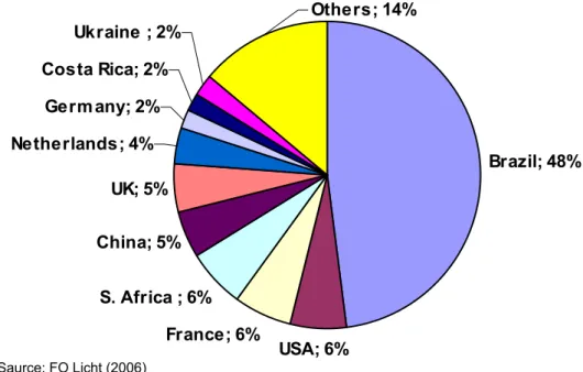
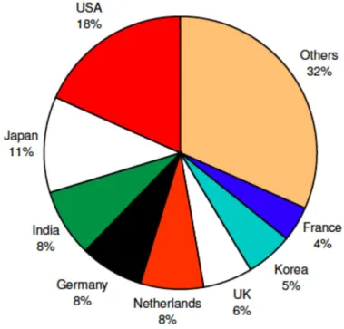
The fuel ethanol market is not mature and is very dynamic. There is not yet a global fuel ethanol market with a spot price and free trade. Multiple uses of feed-stocks also make trade-flows very difficult to trace (GBEP 2008). Traded ethanol made up no more than 10% of global production in 2005 and Brazil was by far the main exporter (IEA Bioenergy 2007). Figure 3 8 below gives an overview over the main exporters of ethanol in 2005 and Figure 3 9 shows the main importers.

Brazil; 48% USA; 6% France; 6% S. Africa ; 6% China; 5% UK; 5% Netherlands; 4% Germ any; 2% Costa Rica; 2% Others; 14% Ukraine ; 2%

Figure 3.8: Main exporters of ethanol in 2005. (IEA Bioenergy 2007) Saurce: FO Licht (2006)

(29)

Figure 3.9: Main importers of ethanol in 2005. (IEA Bioenergy 2007)

The information regarding trade in biofuels should not be regarded as 100% reli-able since the system is under development and much statistics are rather informal (GBEP 2008).

The low level of trade is to a large extent due to high tariffs (International Food & Agricultural Trade Policy Council 2006). USA imported 653.3 million gallons of ethanol in 2006, almost exclusively from Brazil and 1/3 of this ethanol was im-ported through the Caribbean (de Gorter and Just 2008). The United States-Caribbean Basin Initiative (CBI) allows for duty free imports of biofuels from the Caribbean region, if at least 50% of the feedstock is locally produced. The treaty is however limited in that it may only supply up to 7% of the US-market duty free (GBEP 2008). This limit is far from met and there are several refineries under con-struction in the region. They import hydrous ethanol from Brazil and refine it for further distribution to the USA (GBEP 2008).

There is currently no WTO trade agreement in biofuels. Instead they are treated in the General Agreement on Tariffs and Trade (GATT 1994), which covers trade in all goods (GBEP 2008). Discussions are ongoing about whether biofuels should be regarded as agricultural or industrial goods, which is important since governments have much more room to manoeuvre for agricultural goods than for industrial goods, due to some exemptions from free trade agreements (GBEP 2008).

(30)

3.2 Connections between ethanol expansion

in Brazil and the USA: a useful example

to learn from

3.2.1 Land use dynamics: Partial equilibrium models

Modelling the global markets for agricultural products and their indirect effects on biofuels’ mitigation benefit is very complex and results are uncertain (Renewable Fuels Agency 2008). Searchinger, et al., (2008) – published in the journal Science and receiving much attention – used a worldwide partial equilibrium agricultural model to estimate emissions from land-use change and found that maize ethanol, instead of producing a 20% savings (compared to gasoline), nearly doubles green-house emissions over 30 years and increases greengreen-house gases for 167 years. The study is illustrative of the potentially large influence that indirect effects can have on the mitigation benefits of bioenergy initiatives and therefore deserves specific consideration in the context of this report.

The Searchinger article also initiated a debate in the academic community regard-ing indirect land use change (ILUC) and thus the environmental performance of bioenergy in general. However, it should be noted that it has long been recognized that the establishment of bioenergy plantations can lead to changes in the bio-spheric carbon stocks and the land use dynamics and related carbon flows has been studied earlier (see, e.g., (Leemans, et al. 1996) (Berndes and Börjesson 2002)). The recent debate on risks of biospheric carbon losses – which is also the focus of this report – is relevant for the case of conventional food/feed crops expanding into ecosystems with large carbon stocks. But bioenergy systems can also induce in-creases in biospheric carbon stocks. Bioenergy production can be integrated with agriculture in many different ways to deliver environmental services, such as car-bon sinks.

In an article in the recently published book Sugarcane ethanol: Contributions to

climate change mitigation and the environment, Nassar, et al., (2008) investigate

the expansion of sugarcane based ethanol production in Brazil, with a focus on economic; social; as well as environmental effects. They also use a partial equilib-rium model but reach fundamentally different conclusions and claim that there is no LUC or ILUC giving rise to GHG due to expanded ethanol production, mainly taking place in São Paulo state.

To give some perspective on the methodological approaches used by Searchinger and Nassar, a critical assessment of the models is given below with an account of how they differ and what made them reach opposite conclusions.

3.2.1.1 SEARCHINGER’S MODEL STUDY

Searchinger, et al. (2008) used a partial equilibrium model where indirect land use change (ILUC) and other dynamics are modelled as responses to economic

(31)

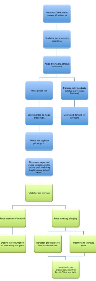
incentives. Using 2004 as base year, almost twice the mandates for ethanol for 2016 is added to get an estimate of how much maize would be diverted from its current use to ethanol production. This increase in diverted maize has two side effects, domestic maize prices increase and the produced volume of by-products such as dry distiller grains (DDGS) rise. Rising maize prices create incentives for farmers to (i) divert suitable land from other uses into maize production; (ii) ex-pand into set aside land (or other land) and (iii) change crop rotations into mono-cropping maize, at the expanse of mainly soybean and wheat production. DDGS can be used for the same purposes as soybeans and can thus reduce the demand for soybeans to some extent. Searchinger, et al. (2008) further assume that there will be a demand for all the by-products produced from the ethanol industry.

The decreased production of wheat and soybeans leads to increased prices for these crops, although the increased DDGS supply somewhat mitigates the price increase. These increased prices reduce the exports of wheat, maize, soybeans, chicken, pork and dairy, whereas beef exports increase somewhat in the model. Food prices in-crease in their study – even at the global level – and producers and consumers re-spond according to their short-term price elasticities (Sylvester-Bradley 2008). On the consumer side there is a small decline in food consumption, mainly in develop-ing countries, and on the demand side the response is to replace the diverted sup-ply. Higher prices provide incentives for farmers to increase inputs to get higher yields at the same time as it becomes profitable to produce crops on lower yielding land. Searchinger, et al. (2008) assume that these effects will be equally large and average crop yields will remain constant for each country in the study. Figure 3 10 shows an overview over the main steps taken in Searchinger’s approach and how the different dynamics influence each other.

Crop yields in the USA are relatively high and most other crop producing countries have lower yields, which imply that the replacement of land is not 1:1 but there will need to be larger areas dedicated to the compensating crop production than the initial area diverted in the USA (Searchinger, Heimlich, et al. 2008).

Searchinger, et al. (2008) have further steps where carbon release from the ILUC is calculated for the different regions. The resulting greenhouse gas emissions are allocated on the expanded maize ethanol in the USA and the time needed for con-tinued ethanol production before the carbon balance becomes equal to gasoline is calculated. These last two steps are omitted from Figure 3.10 because they are not part of the economic dynamic which is in focus here.

(32)

Figure 3.10: The main steps taken in Searchinger's model. The blue boxes symbolize national dynamics (under direct influence by the US), whereas the green boxes symbolize global dynamics that are only indirectly influenced by US decisions.

(33)

Some critical considerations.

Searchinger’s model highlighted several important aspects regarding biofuels, aspects which until then had been overlooked or ignored by scientists as well as decision makers. These aspects of ILUC initiated a heated debate in the academic as well as political world and the study has received a lot of critique regarding their assumptions and methods. There has also been several other studies conducted in response to Searchinger’s study, some which have reached similar conclusions and some which have reached fundamentally different conclusions. Below in this sec-tion is some of this critique is presented and in secsec-tion 3.2.1.2 a different model is presented.

Wang and Haq (2008) criticized the quantitative assumptions made by Searchinger et al. (2008), e.g. about the use of 30 million gallons of ethanol in 2016 instead of the mandated 15 million and also the low mitigation benefit of maize ethanol with no improvements over time and too low feed crop displacement of the DDGS. They further criticized the low level of carbon leakage from soils; the carbon leak-age was also criticized by Dale (2008) in that generalizations regarding soil carbon levels cannot be made. Wang and Haq (2008) further claimed that the US export level of maize can be maintained even if the mandate of 15 million gallons will be reached.

Searchinger (2008) replied to the above raised critique that the absolute amount of ethanol produced is irrelevant in the study since it looks at the marginal effect of an extra gallon of ethanol and not the total emissions. He further claimed that the displacement of DDGS depend on the type of livestock and is very difficult to estimate. Regarding the export levels Searchinger (2008) replied that the export levels can be maintained, but at the cost of reduced export of wheat and soybeans.

There has also been critique regarding the qualitative approach, e.g. that trying to estimate secondary and tertiary effects on the global economy from such a small perturbation is nothing but speculations (Dale 2008). Dale (2008) further claimed that the environmental impacts from ethanol differ between production sites and that local LCA data should be used since American farmers cannot influence for-eign decision makers. Another critique made by Wang and Haq (2008) is that a partial equilibrium model cannot catch all the relevant dynamics from such a com-plex system and that a general equilibrium model, taking supply and demand of agricultural products and land into account, must be used. Khosla (2008) meant that logging is the main driver for deforestation and that bioenergy expansion is more likely in other regions than in forests. The complexity behind deforestation commented on by Kline and Dale (2008) where they emphasized that

“…interactions among cultural, technological, biophysical, political, economic, and demographic forces within a spatial and temporal context rather than by a single crop market…” should be taken into consideration in order to explain the

(34)

Dale’s (2008) perspective is very different from Searchinger’s when he emphasizes on energy security and the first order effects. Using local data for LCA does not take time or scale effects into account, which can be very relevant for an up scaling of a large system over a long time. Background systems change over time, which alters the environmental performance and impacts from a system (Börjesson 1996). Searchinger responded to Kohsla that even though logging takes part in deforesta-tion, the logging is selective and does not clear forests and regrowth of forests normally occur after logging or fires except when agriculture expands onto the land. In the response to Wang and Haq (2008) Searchinger (2008) explained that using a general equilibrium model would not change anything for the marginal gallon of ethanol, since the only difference would be a shifted baseline. Higher yields etc. would change the total impact, but not the marginal effect.

Further critique involves the notion that the approach fails to take polices prevent-ing deforestation, as well as trade agreements into consideration (Renewable Fuels Agency 2008). Searchinger et al. (2008) also receives credits for introducing im-portant aspects but it is also noted that much more research on the topic will be needed (Sheenan 2008).

3.2.1.2 NASSAR’S MODEL STUDY

To evaluate the environmental performance of sugarcane ethanol Nassar, et al., (2008) made a thorough analysis the expansion of sugarcane all over Brazil and what types of land-uses it displaces in order to evaluate the direct land use change (LUC). The analysis is performed in three separate ways by using data from remote sensing satellites, environmental licensing reports and secondary data based on planted and harvested area (Nassar, et al. 2008, p. 64) to assess the impacts from historic expansion. They also create a partial equilibrium model with endogenous demands and prices with which they project the expansion of sugarcane production as well as expansion or reduction of other affected crops between 2008 and 2018. They also have a qualitative discussion regarding ILUC.

The results from the analysis of historic expansion indicate that the most of sugar-cane expansion has taken place on land previously used for food crop production or for cattle grazing and only a very small fraction of the expansion was taking place on virgin land. Carbon losses to the atmosphere due to direct LUC is thus very small or there can even be a net carbon sequestration since sugarcane can bind as much or more carbon as some food crops or degraded pasture (Gibbs, et al. 2008).

For projection of future expansion of sugarcane ethanol Nassar, et al. (2008) use a partial equilibrium model which still is under development by the International Trade Negotiations (ICONE) (Nassar, et al. 2008, p. 73).The model is based on demand and supply responses to changes in prices and returns on production. Mar-ket clearing prices on national or regional level are achieved when supply and de-mand prices coincide (Nassar, et al. 2008, 73), there is however no information of how they calculate the demand and supply curves for the model.

(35)

They use time-steps of one year and a time horizon of 10 years for which they calculate supply and demand for 11 product categories (sugarcane, soybean, maize, cotton, rice, dry beans, milk, beef, chicken, eggs and pork). Unlike Searchinger, et al., (2008) they do not look at global dynamics and the model is confined to Brazil, which is divided into six regions according to biome.

Prices and demands for the products are exogenous for the model and taken from the FAPRI (2008) U.S. and World Agricultural Outlook. The area required to meet these demands for each crop (and sugarcane) is calculated according to yield trends (Nassar, et al. 2008, p. 74). Brazil thus act as a price-taker for all crops as well as ethanol in the model and the expected demand for all products are fixed, even though according to FAPRI (2008, p. 381) the global ethanol price is set mainly by the production level in Brazil.

According to historic data they define a competition matrix between activities with elasticity for change, which later shows results in land-use change distribution between regions depending on the amount of land allocated for each activity (Nassar, et al. 2008, p. 74).

The results from the model show that the total production area will increase for all crops, including sugarcane, but this will be compensated for by a reduction in graz-ing area (Nassar, et al. 2008, p. 84). They further conclude that future expansion of sugarcane will follow the same pattern as in the past, which is not very surprising since they used historic data to calculate their land competition matrix. The use of historic data for expansion patterns can however be well warranted considering the large difference in scale between grazing and cropping areas in Brazil, compared to the ''small perturbation'' from the ethanol industry. Sugarcane expands onto crop land and pasture and most of the displaced crops in turn expand onto pasture land. The pasture area is expected to reduce in all regions except for the Amazon Biome where it expands, but they claim that this expansion takes place without correlation to the reduction in pasture area in other regions (Nassar, et al. 2008, p. 86).

Nassar, et al., acknowledge the problems with defining and calculating ILUC and that especially in a case where the production of sugarcane is taking place far away from the agricultural frontiers and at the same time as the production levels of other (displaced) crops increase. They point out the difficulty to establish causal chains in such dynamics and call for the necessity of searching for “arguments and data

supporting the idea that sugarcane expansion is leading to an increase in the land productivity, rather than promoting incorporation of new land for food production, as grains and pasture land are displaced” (Nassar, et al. 2008, p. 88).

With numbers showing larger displacement of food crops and pasture by sugarcane than the expansion of the same in the Amazon and the fact that food crop as well as meet and dairy production are increasing more than sugarcane, they claim that

(36)

ILUC cannot be quantified and is more than compensated for by yield increases and higher stocking rate.

3.2.1.3 DISCUSSION: SUITABILITY OF PARTIAL EQUILIBRIUM MODELS

Searchinger’s study concerns important aspects that have been ignored by many. The focus on the marginal effect of an extra litre of ethanol production in relatively static surroundings makes the partial equilibrium model appropriate, although the exact numbers reached can be questioned. It can be discussed whether the study (including methods used) directs the public attention in the right direction and in-duce sound processes. For instance, presently developing implementation of energy and climate policy and regulation in EU and USA calls for quantification and as-signment of indirect land use change emissions to specific bioenergy chains, but this cannot (yet) be done with very high level of confidence due to lack of data and methodology verified as sufficiently well reflecting reality. Recently, there was also a decision in California that quantification of ILUC emissions and assignment of those emissions to the ethanol production system will not be allowed until knowledge has improved.

There are some fundamental problems with equilibrium models, namely that they always assume totally homogenous agents and they only include the dynamics the programmer(s) put into the models. Normally modellers are aware of and consider the most important dynamics, but there may be some important factors that are intentionally or unintentionally omitted. Considering how diverse the results can be from such models (as the two assessed studies above show) one can conclude that there is far from agreement on how these dynamics work.

Both Searchinger, et al., (2008) and Nassar, et al., (2008) use historic data to con-struct their land-use-change equations and thus implicitly presume that the future distribution in land use change will be the same as historically has been. Yet his-toric data are more likely to be close to the truth than what a random guess would be, but this approach does not allow for any innovation, changes in behaviour, newly implemented laws, or paradigm shifts in general.

A partial equilibrium model does not include all dynamics in the world (which of course would never be practically feasible to achieve) and thus work in a static surrounding where all else is assumed to be equal. In the current situation with rapidly growing economies in the most populous countries in the world, such an assumption is not likely to be valid.

Nevertheless, Searchinger’s study clearly shows that land use change emissions can drastically reduce the mitigation benefits of biofuels that are based on using food/feed crops as feedstock (such as maize ethanol in the USA) if policies induce a large and rapid increase in inelastic biofuel demand leading to cropland extension into natural ecosystems containing significant carbon stocks. What the model does