Eco‐driving? A discrete choice experiment on valuation of car
attributes
1Martina Högberg, Lund University, Master Thesis in Economics, September 2007 Supervisors: Krister Hjalte2 & Henrik Andersson3
Abstract
To elicit the value that car consumers place upon environmental concerns when purchasing a car, a certain type of Discrete Choice Modelling called Choice Experiment was used. The Choice Experiment includes the four car attributes safety, carbon dioxide emissions, acceleration and annual cost. The survey was sent to a random sample of 1500 people in Sweden between 25 and 50 years of age in October 2006. The data collected was incorporated in a binomial logit model from which the coefficients of the utility function for cars were estimated. Both the estimated values of Willingness to Pay and the Marginal Rates of Substitution gave indications that the private goods safety and acceleration are higher valued than a genuine public bad such as carbon dioxide emissions. The result also showed that the design of the Choice Experiment can have impact on the values obtained.
Keywords: Willingness to Pay, Discrete Choice Experiment, Environmental Valuation
1 The financial and administrative support from Banverket, the Swedish National Road and
Transport Research Institute (VTI), the Swedish Governmental Agency for Innovation Systems (Vinnova), and the National Road Administration (Vägverket) is gratefully acknowledged.
2 Department of Economics, Lund University, Sweden
3 Department. of Transport Economics, Swedish National Road and Transport Research
1. Introduction... 3 1.1 Outline of the study ... 4 2. Theoretical framework... 5 2.1 Willingness to Pay ... 5 2.2 Methods to elicit the Willingness to Pay ... 5 2.3 Choice Modelling ... 7 2.3.1 Choice Experiment ... 8 3. Construction of the survey... 12 3. 1 Survey design... 12 3.1.1 Sample... 16 3.2 Attributes used in the survey... 16 3.2.1 The safety attribute... 16 3.2.2 The environmental attribute ... 18 3.2.3 The performance attribute... 20 3.2.4. The cost attribute ... 20 3.3 Reduction of experiment size... 22 3.4 Test of consistency... 24 4. Results ... 25 4.1 Descriptive statistics... 25 4.1.1 Background data... 25 4.1.2 Car‐related characteristics ... 28 4.1.3 Survey evaluation... 31 4.2 Regression analysis ... 32 4.2.1 Results from basic model estimates ... 33 4.2.2 Results from specific estimations ... 36 5. Discussion... 37 5.1 Basic model... 37 5.1.1 Coefficients ... 37 5.1.2 WTP and MRS... 37
5.2 Specific models ... 38 5.3 Comparison of model results with other survey questions ... 39 5.4 Issues on survey design ... 40 6. Conclusions ... 43 References ... 45 Appendix A: Background material ... 48 Studies on attribute rankings... 48 Applied discrete choice models... 50 Ewing et al, 2000 ... 50 Golob et al, 1997... 51 Lundquist Noblet et al, 2006 ... 51 Appendix B: Model estimations ... 52 Version 1 ... 52 Version 2 ... 53 Version 3 ... 55 Appendix C: Additional questions in the survey ... 58 Appendix D: The survey ... 60
1. Introduction
The environmental problem of global warming has placed itself on top of the agenda. Stricter environmental policies and measures are considered important in order to curb the emissions of greenhouse gases. The transport sector is becoming an increasingly more important emittor. It was responsible for 19 % of global emissions of greenhouse gases in 1971, which had risen to 23 % in 1997 (Åkerman et al, 2006). In 2001, the road transport in Sweden constituted of 29 % of the emissions in Sweden (National Road Administration, 2004).
The trend explains why there is a general agreement on stricter policies needed in the transport sector, particularly focusing on improved energy efficiency. The current voluntary agreement between the European Commission and the European Automobile Manufacturers Association (ACEA), to reduce emissions from newly produced cars to 140 grams of carbon dioxide emissions by 2008 will not be reached, thus probably resulting in a legislatively binding target by 2012. The target will limit the average new car sold in Europe to emit 120 grams of carbon dioxide per kilometre. At present the EU average is at 163 grams per kilometre (The Swedish National Road Administration, 2007).
In Sweden the situation is more troublesome. The country has the most emitting fleet of vehicles in the whole of Europe. On average, a new car sold in Sweden emits 189 grams of carbon dioxide per km, significantly higher than the EU average (The Swedish National Road Administration, 2007). Such a result could be considered to be in conflict with the general view among Swedes of themselves being a people concerned about environment.
The thesis purpose is to answer the following research questions:
1. How much is an individual willing to pay for contributing to lower carbon dioxide emissions when choosing a car?
2. How large is the Willingness to Pay (WTP) for lowered carbon dioxide emissions compared to the WTP for other attributes?
3. Do the preferences for carbon dioxide emissions differ depending on socio‐ demographic characteristics?
The purpose is also to present issues around survey design. There is no attempt made to discuss policy implications of the results.
1.1 Outline of the study
In the next chapter, chapter 2, includes the theoretical framework. The concept of Willingness to Pay is presented, and the different approaches used in order to elicit this value. Further, the particular method used, Choice Modelling is described and why it is appropriate to use for valuation of car qualities. The theory behind the subset of Choice Modelling used in this study, Choice Experiment, is presented. Chapter 3 handles the design of the choice experiment in question. The chapter is extensive due to the fact that there was no prior research performed on the subject and the whole choice experiment and survey had to be designed from zero. Chapter 4 presents the results. It presents the results both from the descriptive statistics in the survey and the results from the regression estimates of the Choice Experiment. In Chapter 5 the results presented in the prior chapter are analyzed more profoundly and discussed. Chapter 6 gathers conclusions from the survey and suggests areas for future research.
2. Theoretical framework
The chapter will explain basic concepts needed to use a Choice Modelling approach to elicit the value that WTP can take for certain attributes of a good, in this case, a car.2.1 Willingness to Pay
The concept of WTP is defined as the amount an individual is willing to pay to acquire a particular good or service. A value on WTP is needed in a case where no market of the good exists and consequently the good has no explicit price. To reveal the WTP is crucial in order to maximize welfare for society as a whole. Environmental goods, which are goods without explicit market prices, have to be given economic values in order to optimize the allocation of scarce resources. This explains why economists during the last thirty years have tried to place monetary values on these (Alpizar et al, 2001). A car is a good sold on a market with an explicit price. However, the purpose is to find the WTP for particular attributes of cars, which separately have no explicit prices. The most relevant attribute of the study is that of lower carbon dioxide emissions for people purchasing cars. The WTP value will be compared to values obtained for other car attributes.2.2 Methods to elicit the Willingness to Pay
Two broad approaches can be applied to determine the value which people place upon non‐market assets: revealed and stated preferences techniques. When relying upon revealed preferences in the valuation exercise, economists use market information and behavior related to traded goods in order to infer values of non‐market goods. The connection to real life actions is the main advantage of the method and thus it should be used when WTP can be inferred from an individual’s actual decisions. Revealed Preference techniques have previously been used to elicit WTP for car attributes (see Andersson 2005 ‐ Atkinson et al, 1990 – Dreyfus et al, 1995)
However, to obtain sufficient data to indirectly infer the revealed preferences for non‐ market goods can be quite difficult. A car market is a good example of such a situation. It consists of many different models and brands which all have different qualities. The factors that explain why a consumer choose a particular model can be numerous and sometimes not even possible to explain. It could be a matter of personal feeling not possible to incorporate in a theoretical model. Instead, as with the situation of car preferences, hypothetical scenarios can be created in order to try to find the preferences and put a WTP on these. Such a model is called a Stated Preference Method and is becoming increasingly popular for valuation of non‐market goods (Alpizar et al, 2001, Bateman et al, 2002).
The Stated Preference Techniques are separated into two groups: Choice Modeling Techniques (CM) and Contingent Valuation Methods (CVM). Contingent valuation is the most common stated preference method applied. The method is well rooted in welfare economics and has been used for more than 30 years for evaluation of environmental goods. By means of an appropriately designed questionnaire, the respondent is given information on the environmental good or bad, the institutional and policy context in which it is to be preserved or mitigated, and the means by which this will be financed (OECD, 2007). The respondent is asked either how much he/she is willing to pay for a certain level of a non‐market good, or how much he/she would be willing to accept to loose the good. Criticism has been put forward to such a hypothetical setting as it runs the risk to overestimate the WTP for the good in question. First of all, many of these questions are asking for valuation of goods that for most people have no actual monetary value. Hence, it makes it difficult for the respondents to know how to value the good in questions, which could result in an overestimation. Secondly, a situation where the scenario is hypothetical, the respondent knows that he or she will not be forced to pay this money in real life and thus have no incentive to more closely consider if the stated WTP is similar to his or her “real” WTP. This is
particularly obvious in a case with dichotomous choice where the amount of money is stated in advance. Moreover, the model is not suited to deal with cases where changes are multidimensional (Hanley et al, 2001), such as a case where several car qualities are changed at the same time.
To conclude, there are certain obvious drawbacks with the CVM technique in order to elicit WTP values. The method could be used in order to extract a WTP value on reduced carbon dioxide emissions from cars, but would face all mentioned problems of how this value actually could be interpreted and related to reality. In addition, one of the purposes of the study is to analyze the size of the WTP for reduced carbon dioxide emissions in relation to the WTP for other car qualities. Such a result would be more difficult to obtain with a CVM approach. Instead, a model that allows valuation of more than one quality of cars is better suited for the purpose in question. Such models are grouped under the name Choice Modelling (CM) techniques.
2.3 Choice Modelling
Choice Modelling (CM) is the common name for a group of survey‐based methodologies where goods are described in terms of attributes and levels that these take, in contrast to CVM where the good is described as the good itself and thus the WTP is stated directly (Alpizar et al, 2001 ‐ Hanley et al, 2001). Such property explains why the model mostly has been used for marketing purposes.In addition to having advantages of focusing on attributal changes it is considered advantageous as the trade‐off can be expressed in terms of goods instead of in monetary terms, like in CVM. Such a property explains its increased use to value institutional and environmental changes. People tend to feel uncomfortable trading off money for environmental attributes. In a situation where the WTP is inferred indirectly and the respondent need to do a trade‐off, it is more difficult to behave strategically which can decrease the risk of overstating WTP (Hiselius, 2005 ‐ Ryan, 2000).
The Choice Modelling also faces downsides. First of all it runs the risk of creating a cognitive burden for the respondents. Too many attributes and levels included can result in a survey very difficult for the respondents to comprehend. Both experimental economics and psychologists have found evidence that there is a limit to how much information respondents can handle while making a decision. The random errors seem to increase simultaneously as the number of choice set increases (Bateman et al 2003). Thereby, an internal consistency test should be incorporated in the survey (Hanley et al 2001). Secondly, although the model includes a trade‐off situation, it is still sensitive to survey design and that the accurate levels and descriptions are included in the choice sets (Bateman et al, 2002). Hence, the risk to over or underestimate WTP with CM should not be neglected. In order to test for these differences, the Choice Model can include several survey designs.
2.3.1 Choice Experiment
To obtain the coefficients in order to elicit the WTP for carbon dioxide emissions and compare this to the WTP of other car qualities, a certain type of CM is used, called Choice Experiment (CE). It is a subset of the CM technique and has mainly developed within the field on transport and environmental economics (Ryan et al, 2000). In a CE, the respondent is presented to a number of discrete choice situations and asked to choose the most preferred. One scenario is typically defined as the status quo (defined as no buy or, alternatively, to stick with the default scenario).
The Lancasterian microeconomic approach is the source of inspiration for the Choice Experiment technique; utility is derived from the commodity attributes rather than the commodity itself. The contribution of each attribute is the part‐worth of the utility function. The choice situation makes it possible to estimate the relative weight of each attribute, i.e. the Marginal Rate of Substitution (MRS) (Hiselius, 2005). By including price/cost as one of the attributes, WTP can indirectly recovered be from the choices
made (Hanley et al, 2001). One benefit with CE is that each choice involves explanation of a number or attributes and thus much information can be elicited from each choice situation (Alpizar et al, 2001).
The Choice Experiment builds on the Random Utility Theory. It is based around an alternative theory of choice to that used to derive conventional demand curves (Bateman et al, 2002). An individual J´s utility from a certain car is stated by a utility function where the utility depends on the characteristics, Z, of the car. Some of the characteristics included in Z are not known to the researcher. To illustrate such a situation, the conventional utility function is broken down into two parts, one observable part V and one error part, ε. In addition to the car attributes that the utility function consists of, there are a number of socio‐demographic characteristics, S, as well, which affect both the observed and the unobserved part. The utility function for an alternative A can be illustrated as in equation 2.1. UAJ(ZAJ,SAJ) = VAJ(ZAJ,SAJ) + ε(ZAJ,SAJ) (2.1) When an individual J is asked to choose between two cars (A and B), differentiated by the different levels of the attributes included, the individual is assumed to compare the utility he/she would get from either choice, and select the car giving highest utility, as the individual is assumed to be a utility maximizer. The error term is included as the respondents may assess the options according to information other than shown and thus not possible to elicit from the survey. The list of available options is referred to as the choice set, which in this case includes two alternatives.
Given that an error component is incorporated in the utility function, no certain predictions can be made and the analysis becomes one of probabilistic choice. The probability that individual J prefers car A over car B can be expressed as in equation 2.2.
P[(VAJ+ εAJ) > (VBJ+ εBJ)] = P[(VAJ – VBJ) > (εBJ – εAJ)] (2.2)
This implies that the respondent J will choose car A over car B if the differences in the deterministic parts exceeds the differences in the error parts. For purposes of empirical measurement, a probability distribution is assumed for the error part. It is typically assumed to be independently and identically distributed with an extreme value (Gumbel) distribution, given by equation 2.3.
P(ε≤t) = F(t) = exp (‐exp(‐t)) (2.3)
The distribution of the error term implies that the probability of A being chosen as the most preferred can be expressed in terms of the logistic distribution, known as the conditional logit model, expressed in equation 2.4.
P(UAJ>UBJ) = exp(μVAJ)/∑(expμVBN ) (2.4)
μ is a scale parameter, inversely proportional to the standard deviation of the error distribution. In single data sets this parameter cannot be separately identified. In a case, such as the choice between two cars A and B, a binary model is required. If the dependent variable takes on three values (for instance A, B and “neither of the alternatives”, a multinomial logit‐model (MNL) is required.
The selections from the choice set should fulfil the precondition of Independence from Irrelevant Alternatives (IIA) property, which states that the relative probabilities of two options being selected are unaffected by the introduction or the removal of other alternatives. Whether the IIA is violated can be tested using a procedure by Hausman & McFadden (Hanley et al, 2001, Bateman et al, 2002). Nested Logit Models could be used to deal partially with IIA assumptions (Ryan et al, 2000).
The model can then be estimated by conventional maximum likelihood procedures, which results in estimations of the coefficients of the variables included in the utility function. Marginal Rate of Substitution (MRS) is defined as the negative ratio between two attributes. When one of these is the cost attribute, the ratio is called the marginal WTP, illustrated in equation 2.5.
WTPattribute = ‐βattribute/βcost (2.5)
The ratio between any other attributes is showed in equation 2.6.
3. Construction of the survey
One of the most challenging tasks in a choice experiment is the experimental design, where the investigation problem is specified and the survey designed. This is particularly true here, as no similar surveys have been made prior to this. The biggest difference to earlier studies is that this study does not compare environmental attributes with each other, but does instead compare environmental attributed to other car related characteristics. Such a case is interesting, as it means that the WTP for private attributes are compared to the WTP for public attributes. Furthermore, earlier studies have not been unlabelled. To perform an unlabelled study could minimize problems with errors included in the intercept variable. As this work touches upon completely new areas of research, a great deal of the paper explains the background work of the design of the survey. The design process is based on the theoretical parts presented in Hensher et al (2005), Alpizar et al, (2001) as well as Bateman et al, (2002).
3. 1 Survey design
In addition to mentioned literature used for the survey design, earlier studies on ranking of car attributes were used to find the most relevant attributes to incorporate in the model. The few earlier CM studies found were also used as reference material. (see Appendix A for a more complete description of the background material). In August 2006, a small pilot study was performed to test the model.
In the choice model, four car attributes is incorporated: safety, carbon dioxide emissions, acceleration and annual cost. The number of attributes was reduced to four after a pilot study with five attributes proved to be complex for the respondents. There is always a trade‐off between the risk of leaving out attributes considered essential for the consumer, and the benefit of a low task complexity. The attribute NOx emissions was
removed from the final design as it was not considered to outweigh the increased complexity.
In addition to include important attributes, an important precondition for the choice is the possibility of measurement, where “softer” attributes such as comfort, status and road performance often are quite difficult to measure. A compromise between possibility to measure and straight forwardness has to be made (Hensher et al, 2005).
Surveys indicate1 that safety is considered a crucial attribute both for Swedish and European car consumer and it was therefore included in the survey. As the study is focused on carbon dioxide emissions, such an attribute is included. These are supplemented with a third attribute called acceleration. It is considered important for consumers as a way to explain speed qualities and engine size. In addition, it is to some extent in conflict with both safety and environmental considerations, which improves the need for the respondent to face a real trade‐off situation. The fourth and last attribute is cost, necessary to derive the WTP.
In total, three different survey versions were created. The respondents were randomly handed one of these. Three versions were made in order to give the opportunity to perform further analysis of the Choice Experiment methodology and to study what impact the survey design can have on the final result. Such aspects are not profoundly studied here, but the data material allows for more studies of that kind to be performed. The attributes are all given five levels in the basic design, called Version 1. The levels are linked to the real life situation in order to produce cleaner data, preferred for modeling purposes (Alpizar et al, 2001, Hensher et al, 2005). Version 2 was identical to version 1, in everything except that the cost levels were halved. The idea is to test how the cost
levels used affect the obtained WTP values. It is possible that the respondents are more concerned by the relative value of the cost, especially when the levels also are illustrated in a figure, than the actual absolute value presented. In Version 3, all attributes except cost were only presented with three levels, where the two extreme values in the basic case are excluded. The purpose is two‐fold. Firstly, the motive is to see whether fewer levels improve the possibility to understand the question and to make a choice. Such a case would be seen through a greater number of complete answers compared to version 1 and 2. Secondly, only using three levels should test for the sensitivity to scale through the way values are presented. In theory, a respondent should have the same WTP for, for instance, 140 grams of carbon dioxide ‐ independently of whether this level is illustrated as the lowest level, as in version 3, or as the second lowest level, as in version 1 and 2. However, the way the choice sets are illustrated, the respondent might take less notice of the absolute levels that describes the car and is instead more focused on how this level is described in reference to the other levels.
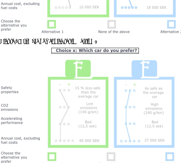
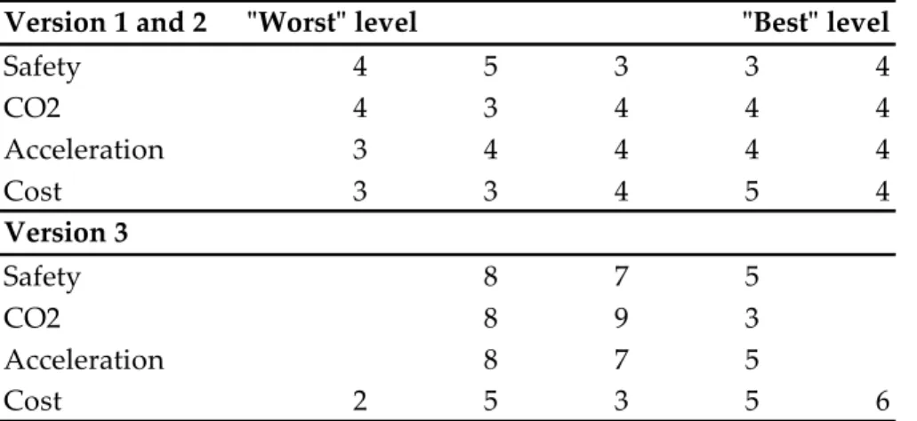
As it proved difficult to create a status quo scenario for cars, the final choice was to not incorporate such an alternative, despite its obvious advantages. Simply not everyone drives the same type of car with the same properties. Instead binary choice sets are used, complemented with a no‐choice alternative. Unrealistically forcing decision makers to select among the two alternatives could inflate the estimates obtained (Hensher et al, 2005). Figure 1 and 2 shows examples of choice sets in Version 1 and Version 3.
Figure 1: Example of choice set in survey version 1
1
Choice x: Which car do you prefer?
2
The safety property of the car The CO2 emissions The accelerating performanceAnnual cost, excluding fuel costs
1
15 % less safe than the average car Low emissions (140 g/km) Good (7,5 sec) 10 000 SEK2
30 % less safe than the average car Bad (12,5 sec) 18 000 SEK Very low emissions (90 g/km)-
+
-
+
Choose the alternative you preferAlternative 1 None of the above Alternative 2
Figure 2: Example of a choice set in Version 3
Choice x: Which car do you prefer?
Safety properties CO2 emissions Accelerating performance
Annual cost, excluding fuel costs 15 % less safe than the average car Low emissions (140 g/km) Bad (12,5 sek) 40 000 SEK
2
As safe as the average car Bad (12,5 sek) 27 000 SEK High emissions (240 g/km) Choose the alternative you preferAlternative 1 None of the above Alternative 2
- + - +
1
The survey was sent out as a mail questionnaire, consisting of 23 questions where question 11 was the Choice Experiment with six its different choice sets. The first ten questions treated information on car preferences to obtain data on plausible purchasing plans, price class of such a vehicle and what attributes the respondent rank highest in a car. Five safety attributes were also ranked in order of importance. Lastly, the respondent stated which fuel type it thought was best in order to cumber climate change. The survey ended with socio‐demographic variables and some questions giving opportunity for evaluation of the survey. The whole survey is found in Appendix D.
3.1.1 Sample
The three different survey versions were in October 2006 sent to a random sample between 25 and 50 years of age, with a geographic spread over the entire country. Each survey version was randomly given to 500 people, giving a total number of 1500 individuals. To target a particular age group was motivated as a way to increase the possibility of the respondents being car owners. As the expected response rate for surveys sent out by mail is around 25‐50 % (Bateman et al 2002) much effort was placed on making a survey appealing and easily understood for the respondent. In addition, a reminding letter was sent after some three weeks. Those that chose to complete the survey were rewarded with a lottery ticket.
3.2 Attributes used in the survey
This section explains the creation of the attributes used in the Choice Experiment.
3.2.1 The safety attribute
The first attribute in the Choice Experiment is safety. There are a number of aspects that have to be taken into consideration when creating a proper safety measurement. The monetary value of safety should preferably be able to translate into a reduction in mortality risk. The value of a statistical life, (VSL) defines the monetary value of a mortality risk reduction that prevents one statistical death. Monetary values for risk
reduction have been used since the 1960s by the National Road Administration in order to evaluate road‐safety policies (Andersson, 2005).
A first problem to tackle is how to define safety. Safety could be a matter of personal feeling; a car could feel safe even though it is not. Moreover, there is a general misconception that a big car is safer than a smaller car. To be able to increase the validity of the measure, subjective differences need to be prevented as much as possible. The second aspect is to whom the safety is applied. It could be driving safety, collision safety or safety for another part (pedestrians, other vehicles etc). This study is restricted to collision safety, and merely for the driver and the passengers in the car. The choice is partially based on the result of a survey conducted by MORI & EuroNCAP2 in 2005, which stated that people do in fact consider safety for the driver and front seat passenger being the most influential safety aspect when choosing a car (MORI and EuroNCAP, 2005). In addition, to create a safety attribute that is a private good, it should be restricted to include safety for the people inside the car.
The third aspect is how to measure safety. One way is to look at the absolute decrease in risk, taking into account the total risk of a fatal accident or a severe injury in an accident. For example, improved safety could be a reduction in the fatal risk from 6/100 000 to 4/100 000. However, as we are facing tiny probabilities, earlier research has shown that respondents tend to be insensitive to scope. It can be difficult to comprehend such a small scale risk and state a correct WTP (Bateman et al, 2002, Rizzi et al, 2005). Thus, it could be beneficial to use a relative measure of safety. A few well‐known safety indicators already exist. In Sweden, the most commonly known are the EuroNCAP and 2 MORI stands for Market & Opinion Research International and EuroNCAP for European New Car Assessment Programme.
the Folksam3 ranking. EuroNCAP is based on simulated crash tests for new cars, where the performance is graded with one to five stars. The Folksam measure is based on statistics from real life accidents, where the cars are ranked on a scale from more than 15 % less safe than the average car to 30 % more safe than the average car. The Folksam indicator was used in the survey, complemented with information of the absolute risk of a fatal accident (5/100 000 per year) stated in the attached information sheet. Figure 3: Safety levels in survey version 1 & 2: 30 % less safe than the average car 15% less safe than the average car As safe as the average car 15 % more safe than the average
car
30 % more safe than the average
car
The safety levels presented in Figure 3 are based on the levels used by Folksam (2005), based on real accidents registered. The levels were modified somewhat as the real life indicator includes both risk for severe injuries and fatal accidents. In the survey it is explained to the respondent that the levels demonstrate the risk for fatal accidents. Attached to the description of attribute levels, the annual absolute risk for a fatal accident was included to make sure the respondent gets a good perception of the risk measure.
3.2.2 The environmental attribute
The main purpose of the study is to find a WTP value for lower emissions of carbon dioxide. At the beginning of this work, the idea was to compare lower emissions of carbon dioxide to other environmental concerns, such as the emissions of NOx and particles. However, the pilot study that included a NOx emissions attribute, turned out to be too complicated for the respondents. Thereof, the final study only includes carbon dioxide emissions, as this environmental problem is the most evident related to cars
nowadays. In addition, newer cars do often have engine techniques which remove particles and other emissions.
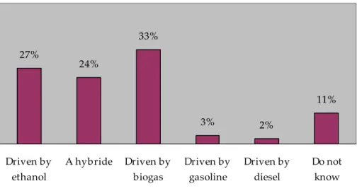
In the survey, the environmental attribute consists of grams of carbon dioxide emitted per kilometer. This to make the attribute technology neutral, i.e. it does not relate environmental classification of the fuel type used. It could be a conventional diesel or gasoline car, a hybrid, or even a car driven by alternative fuels, although their carbon dioxide emissions are harder to quantify. By using the simple measure grams carbon dioxide per kilometer, there is no need to take into consideration what type of fuel or car technology that is actually best for the environment, in a climate change perspective.
The indicator carbon dioxide emissions per kilometer is frequently used. For instance, in the present agreement with ACEA the target is to reduce the emissions of carbon dioxide to 140 g/km by 2008. In addition to these advantages, the attribute is expected to be easily understood by the respondent, where the levels are stated clearly in a cardinal scale. Figure 4: Levels of carbon dioxide emissions in survey version 1 & 2 Very lo w em issions 90 g/km Lo w em issions 140 g/km Averag e em issions 190 g/km High em issions 240 g/km Very high em issions 290 g/km As seen in Figure 4, five absolute levels of carbon dioxide emissions were used, that ranges from 290 g/km down to 90 g/km. All these levels are feasible at present. The average value corresponds to the average of a new car sold in Sweden. Only a few newly produced cars can reach the lowest emissions, 90 g/km, whereas there are cars with emissions up to 450 g/km or more (The Swedish Consumer Agency, 2006).
In this leveling, plausible lower net‐emissions from cars using alternative fuels like ethanol and gas are not considered as the net emission estimations are unclear, depending on the share of bio fuel used for driving. A hybrid like Toyota Prius, falls into the level interval with 104 g/km (ibid). As seen here, the levels used are based on national values. That 190 g/km is the average value in a Swedish context, whereas it would be a high value in a European context, does entail that the results have to be considered in a national perspective.
3.2.3 The performance attribute
The surveys in the relevant literature revealed high impact of road performance/road holding and running reliability. To represent such an attribute, acceleration is chosen. It is easily leveled and can be stated in numbers. In addition, the acceleration indicator is commonly used in car commercials to explain its engine power. The acceleration attribute is not covering all criteria on performance, but was found most appropriate for this purpose. It indicates the time it takes for the car to accelerate from 0 to 100 km/h ‐ the shorter time, the better acceleration. The levels showed in Figure 5 are based on real life data on acceleration of new cars provided by the Swedish Consumer Agency in April 2006. Figure 5: Levels of acceleration in survey version 1 & 2 Good (7,5 sec) Average (10 sec) Bad (12,5 sec) Very bad (15 sec) Very good (5 sec)
3.2.4. The cost attribute
A cost attribute is included to be able to state WTP in monetary terms. According to Bateman et al, 2002, the price tag needs to be credible and realistic, and should ideally minimize incentives for strategic behavior. It should be commensurate with the levels of
the attributes; prices that are too low will always be accepted and result in a small price coefficient. Vice versa, prices that are too high will always be rejected.
The car cost consists of many different parts: Vehicle purchasing cost, fuel cost per kilometer, insurance cost, reparation cost and maintenance cost, to mention a few. In this study, the annual cost of the car is used, which here includes depreciation rate, insurance, and tires, but excludes fuel consumption costs. The inclusion of fuel costs could interfere with the environmental attribute as it induces considerations on distance driven and consumption per kilometer. Annual cost is preferable over a cost such as purchasing cost, as it is limited to a certain time period and thus does not have to take discount values into consideration. Moreover, both the costs and the gains (safety, environment and acceleration) need to be included in comparable periods of time, in order to know the trade‐off situation.
Another benefit in using annual cost is that it removes difficulties with large price differences between newer and older cars. If purchasing cost would be used, it would run the risk of being either too expensive for the persons only interested in buying second hand cars and vice versa, as it would not take into consideration people wanting to buy the most expensive cars if these were not included. With annual costs, the cost interval becomes smaller than with an initial purchasing cost.
Figure 6: Levels of annual cost in survey version 1 & 3
55 000 SEK 40 000 SEK 27 000 SEK 18 000 SEK 10 000 SEK The attribute levels in Figure 6 are based on a web tool on the Swedish Consumer Agency website, where it is possible to calculate the annual cost on certain car models (Bilkalkylen, April 2006). Almost the entire cost span which was found is included in the interval used here. Version 1 & 3 include identical cost levels, whereas the version 2 has halved cost levels, showed in Figure 7.
Figure 7: Cost levels in survey version 2
27 000 SEK 20 000 SEK 14 000 SEK 9000 SEK 5 000 SEK
3.3 Reduction of experiment size
After deciding how many attributes, levels, alternatives in the choice set, number of choice sets and the number of survey versions, it is necessary to design a statistically efficient subset of possible alternative combinations (Bateman et al, 2003). The full factorial design in version 1 and 2 generates 5*5*5*5= 625 number of combinations and Version 3 generates 3*3*3*5= 135 combinations of the attributes. The standard approach has been to identify four criteria for the efficient design (Alpizar et al, 2001): 1. Orthogonality. The combinations chosen should be those where the variations of the levels of the attributes are uncorrelated in all choice sets. 2. Level balance. The level of each attribute should occur with equal frequency in the questionnaire. 3. Minimal overlap. The attribute level should not repeat itself in the choice sets. 4. Utility balance. The utility in each of the two alternatives in the choice set should
be set equal. This to be able to extract the best available information from each choice set. The disadvantage is the increased difficulty that this implies for the respondent (Alpizar et al, 2001).
In order to create an orthogonal design, the statistical package SPSS was used. 25 combinations of the attributes and attribute levels for the set to be orthogonal were created. Although orthogonality is a desirable property in a choice task design, there are practical reasons to depart from it (Bateman et al, 2003), which was the case in this survey. The levels presented have to be realistic and plausible. Based on that, several combinations were removed from the design. After removing unrealistic combinations,
each of the survey versions 1, 2 and 3 included 20 combinations of the attributes. Each choice set included two sets of combinations, creating a total of 10 choice sets for each survey version. However, as 10 choice sets were considered too many for each respondent to handle, the combinations in each survey version were divided into two separate surveys. Thus, the set of 500 respondents provided with each survey version was divided in to two parts, giving 250 individuals receiving exactly the same choice sets.
When creating the choice sets from the attribute combinations, focus was placed on the utility balance (criteria 4), in order to prevent any of the alternatives to become dominant. This property was seen as most important, as the larger the difference in utility between the alternatives, the less information is extracted from the specific choice set (Alpizar et al, 2001). But as some of the combinations had been removed it was a problem to maintain the minimal overlap and the level balance.
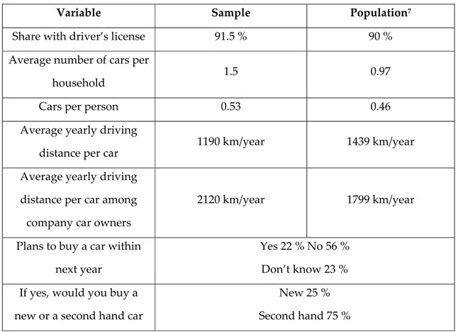
Table 1: Level balance after reduction of experiment size and the choice set creation Version 1 and 2 ʺWorstʺ level ʺBestʺ level
Safety 4 5 3 3 4 CO2 4 3 4 4 4 Acceleration 3 4 4 4 4 Cost 3 3 4 5 4 Version 3 Safety 8 7 5 CO2 8 9 3 Acceleration 8 7 5 Cost 2 5 3 5 6
Table 1 shows the number of times each attribute level is presented in each survey version, 1,2 and 3. As seen, the level balance is not exact in neither of the versions, i.e. each level is not presented an equal number of times, which could create collinearity (Mc Intosh et al, 2002). The five‐levelled version 1 & 2 is however better balanced than
version 3. In Version 3, the “worst” level is presented more times than the “best”. This bias should be studied further, but is out of scope of this study.
3.4 Test of consistency
As mentioned in section 3.1, each participant was given six choice set, to not make it too demanding. Five of these were combinations created in the orthogonality design. The sixth choice set was an internal test of consistency.
An individual is rational when its preference ordering is complete, reflexive, transitive and continuous. If these are fulfilled, the individual’s preferences can be represented by a utility function. (Mc Intosh et al, 2002) This survey merely included a test for transitivity. The sixth choice set was duplication of the first, but with changes in the attribute levels in one of the alternatives. The attributes in alternative A was changed to include more utility, whereas the utility in alternative B was kept identical as in choice set one. If the respondent in choice set one chose alternative A, it should choose A in the sixth, as it is better. Hence, the criteria of transitivity would be fulfilled. If the respondent had chosen A in the first set and then chose B in the sixth, the answer is inconsistent. A drawback with such a test is that only those that had chosen A in choice set 1 could be tested. If the respondent had chosen B in the first choice set and B in choice set 6 nothing could be said. Although A in the sixth choice set was given higher utility than in the first it does not necessarily mean that the respondent will change from B to A. However, if the individual chose the alternative “none of the above” in choice set 1 and then chose B in choice set 6, which had less utility than A, the individual had violated the assumption of transitivity. All responses from respondents who violated the transitivity criteria were removed from the final data set.
4. Results
4.1 Descriptive statistics
This section presents the results from the questions not connected to the Choice Experiment.
4.1.1 Background data
In this section, the sample is described. Table 2 compares the background data of the sample with the same characteristics of the Swedish population as a whole. Table 2: Comparison of the sample data and the population as a whole Variable Sample Number of usable responses 734 Response rate 49 % Population4 Share men 52 % 49.6 % Share women 48 % 50.4 %
Mean age 37.8 years 40.9 years
Median age 38 years 40 years
Resides in city/densely populated area 73 % 77 % Education level upper secondary school
or higher
93 % 84 %
University studies 45 % 35 %
Household income average/month SEK 37 000 SEK 22 000
There is a slight bias towards a higher share of men in the sample, 52 %, compared to 49.6 % in the population. The small difference could be explained by the fact that men to a larger extent own cars than women do and car owners are more likely to respond a
survey treating car preferences. In the end of 2006, 66 % of all privately owned cars were owned by a man (SIKA Fordonsstatistik5). Due to this it is not surprising that the share of men among the respondents exceed the share of men in the population.
The mean and median age of the respondents are somewhat lower than in the population as a whole. However, the sample consisted of people aged 25 to 50 years, which means that the mean value of about 38 years is very close to the expected mean of that particular age group.
In the sample 73 % of the respondents live in densely populated areas. The corresponding share of the population amounts to 77 %, not a great difference.
The respondents tend to possess a higher education level than the national average of the age group. In the sample, 45 % of the respondents have attended some form of post high‐school studies, compared to the national average of 35 %, and the group with nine years of compulsory school is smaller in the sample than in the population, 7 % compared to the national average of 16 %. A possible explanation to the divergence is the fact the people with a higher level of education generally have a higher income and are therefore more likely to have a car. In addition, it could be that more educated people are more interested in responding to such a survey.
The largest difference between the sample and the population is found in average household income. In the sample, average household income amounts to SEK 38 000 per month, compared to an estimated average income of SEK 22 000 of a Swedish household6.
5 Statistics from the Swedish Institute for Transport and Communications Analysis 6 In the SCB statistics there are only numbers for disposable income.
Figure 8: Distribution of household income in sample Household income 3% 14% 39% 33% 12% 0 ‐10 000 SEK 10 001 ‐ 20 000 SEK 20 001 ‐ 40 000 SEK 40 001 ‐ 60 000 SEK 60 001 SEK or more
As seen in Figure 8, the majority of households in the sample have an income level above SEK 20 000 per month. It is obvious that the sample respondents consist of a higher share of high income households than the population average. The underlying reasons are several. At first, the age group included in the sample is 25‐50 years, whereas the national estimation also includes senior and younger citizens – age groups that often have lower incomes. Secondly, there is the earlier mentioned divergence towards a sample with a higher proportion of car owners and highly educated people, in turn leading to a higher average income. To summarize, the sample is in several aspects very similar to the population. In despite of a response rate of below 50 %, the only two variables with a significant deviation is average income and education level ‐ discrepancies that have obvious explanations.
4.1.2 Car‐related characteristics
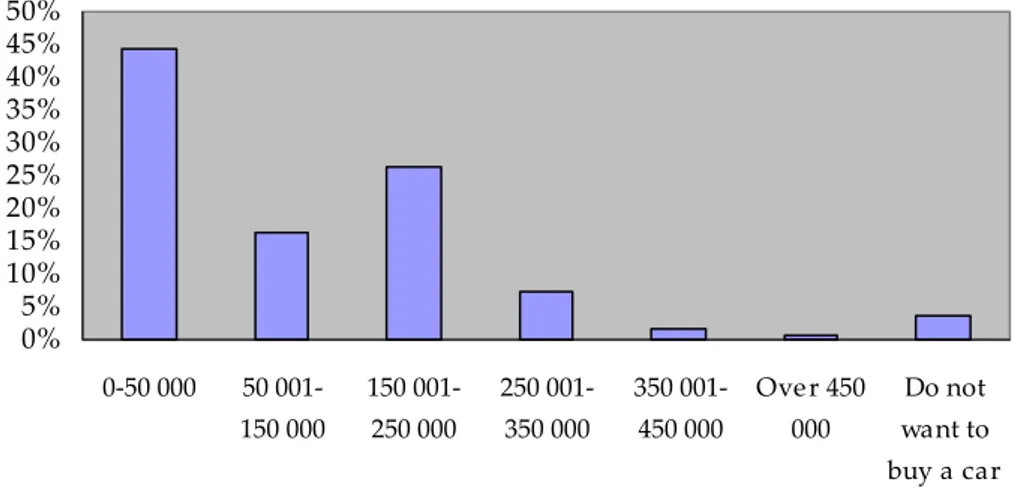
Table 3: Comparison of the sample data and the population as a whole
Variable Sample Population7
Share with driver’s license 91.5 % 90 % Average number of cars per household 1.5 0.97 Cars per person 0.53 0.46 Average yearly driving
distance per car 1190 km/year 1439 km/year
Average yearly driving distance per car among company car owners 2120 km/year 1799 km/year Plans to buy a car within next year Yes 22 % No 56 % Don’t know 23 % If yes, would you buy a new or a second hand car New 25 % Second hand 75 %
An expected bias in the survey was that only persons with a driver’s license would complete it. A person with a driver’s license is more likely to actually own a car, which in turn makes him/her more likely to complete the survey. Table 3 shows that in the age group 25‐66 years around 90 % of the Swedes have driver’s license. The corresponding share in the sample is 91.5 %, which implies that the sample in this context is, if anything, very modestly biased towards respondents with a driver’s license. However, in order to get good results, it may have been more desirable to have a sample only containing persons that can drive a car, as these people probably are more aware of what attributes they prefer in a car.
To further investigate whether the sample is biased towards car‐owners, information on average number of cars per household was provided. In the sample the average number of cars among the respondents’ households is 1.5, compared to the national average of about 1. At first sight it seems as a rather great distortion towards more car‐owners among the respondents completing the survey, but could be explained as a person in the age group 25‐50 can be expected to be part of a larger household and therefore in need of more cars. Moreover, the particular age group could be expected to have a higher income. Such things could explain the higher number of cars per person in the sample.
The average yearly driving distance per car in the sample amounts to 1190 km/year, which is below the national average of 1439 km/year. A shorter driving distance is partly expected since the households in the sample have access to a higher number of cars. An interesting feature is the occurrence of households solely driving a company car. In transport statistics it is a well‐known phenomenon that these types of cars on average have a higher yearly driving distance, a fact that is true also for the sample8. The survey included some questions about the respondent’s possible plans to purchase a car in the future. About one fourth of the respondents stated that they plan to buy a car within a year. Out of these respondents, 75 % planned to buy second‐hand. In addition, the survey contained a question of which price group a newly purchased car would lie within. The answers were distributed as illustrated in Figure 9. 8 Note that the sample only contains 25 households solely depending on company car(s).
Figure 9: Distribution of aimed price groups for car buyers 0% 5% 10% 15% 20% 25% 30% 35% 40% 45% 50% 0‐50 000 50 001‐ 150 000 150 001‐ 250 000 250 001‐ 350 000 350 001‐ 450 000 Ove r 450 000 Do not want to buy a car
Figure 9 illustrates that the majority would purchase a car in the lowest price group. This is an obvious consequence to the statement that a vast majority would buy a second hand car. As a large share of the respondents stated that they would purchase a car in the cheaper price groups, it could be expected that that would have a lowering effect on the final WTP values obtained in the regression analysis part of the study. A question about the respondents’ interest in cars was asked in order to further study the possibility of a bias towards the more car interested part of the population. The answers were distributed as seen in Figure 10. Figure 10: Distribution of car interest among respondents 15% 8% 19% 34% 24% No interest at all Very interested
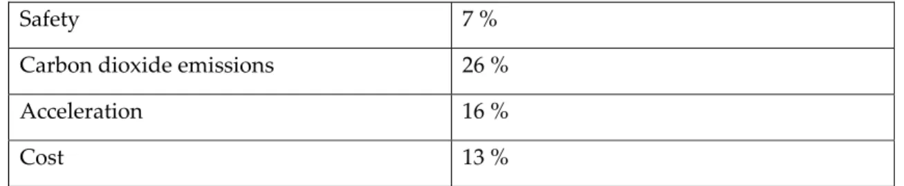
The sample seems to be a rather evenly distributed when it comes to interest in cars as illustrated in Figure 10. Obviously there are difficulties comparing this distribution, as there is no information available of the corresponding distribution among the population. Figure 11: Share of attributes that were chosen as one of the five most important 85% 78% 72% 59% 54% 47% 41% 31% 23% 6% 4% 0% 20% 40% 60% 80% 100% Safet y Runn ing cost s Road perf orm ance Com fort Envi ronm ental pro perties Stow ing Desi gn Bra nd Acc eler atin g per forma nce Luxur y Oth er
Question 8 in the survey asked the respondent to choose five out of ten presented attributes and rank these in order of importance. If the respondent thought an important was missing he/she had the possibility to include it. Figure 11 presents part of the results. Safety was considered most important, being included among the five most important in 85 % of the responses. In addition, out of those who had included it in the five, 42 % had selected safety as the most important attribute.
4.1.3 Survey evaluation
At the end of the survey, two questions of evaluation were included. These revealed that more than 50 % thought it was easy or very easy to complete the survey, whereas only 8 % thought it was difficult or very difficult, while the remaining 42 % chose the average alternative. Moreover, 82 % said that the background information attached wassufficient to answer the questions. The respondents also had the opportunity to add comments to the responses, which merely a small portion of the respondents did.
4.2 Regression analysis
A binomial logit model was used to estimate the coefficients of the utility function for cars, using the Limdep software. As the model actually included three alternatives including the “none of the above” alternative, the experiment could have been estimated using a MNL model. However, the alternatives where the “none of the above” was chosen provided no data for the estimation and was thereof treated identically as the alternatives where no choice was made at all. Thus, all rows with no response at all or where the alternative “none of the above” was chosen were removed and not included in the estimation. This goes against the rules on how to maintain orthogonality in the experimental design, where all the individuals’ choice sets should be removed from the final results if the opt‐out alternative was chosen in one or more of the choice sets. However, this created too few complete responses in order to maintain statistical significance in the result. Moreover, as showed in section 3.3, there was already in the complete design a slight distortion in level balance.
All attributes in the choice set were continuous. The alternatives were generic and not labeled, which gave no extra value of including an alternative specific constant in the model. An unlabelled experiment where the choice is between A & B, where the only difference is the levels of the attributes, A & B does not convey meaning to the respondent on what the alternatives mean in reality. If the choice also had included something like the brand of the car, there could be expected that factor others than shown could be influencing (Hensher et al, 2005).
Intransitive responses were tested for in the sixth choice set. All the respondents that had acted intransitive were removed from the choice experiment; as such answers are inconsistent with basic consumer theory assumptions. Out of the responses, 21 were
intransitive responses, which is less than 3 % of the total number of responses. The highest rate of inconsistent answers is found in survey 2 and 4 out of the six in total (29 % respectively 43 % of all inconsistent answers). The finding is interesting as these versions are identical in everything accept the halved cost levels, but this will not be analyzed further in the study.
It was not possible to create a Nested Logit Model, where only those that plan to purchase a car within a year is included. Only 22 % of the respondents said they planned to buy a car within a year, which was too few in order to create such a model where the statistical significance was maintained. The advantage of only including those planning to buy a car is that such a group solely consist of people that are to perform a similar choice in real life, which can improve the reliability of the result by making sure the IIA criteria, explained in the theory part, is fulfilled.
4.2.1 Results from basic model estimates
Table 4: Estimates from the binomial logit model Version 1 Number of observations: 1342 Coefficient Standard error Safety 0.0107*** 0.00274 Carbon dioxide emissions ‐0.00133** 0.000576 Acceleration 0.0560*** 0.0111 Annual cost ‐0.0000123*** 0.00000314 Version 2 Number of observations: 1362 Coefficient Standard error Safety 0.0168*** 0.00278 Carbon dioxide emissions ‐0.00304*** 0.000546 Acceleration 0.0847*** 0.011 Annual cost ‐0.0000218*** 0.00000641 Version 3 Number of observations: 1498 Coefficient Standard error Safety 0.0115*** 0.00442 Carbon dioxide emissions ‐0.00166 0.00104 Acceleration 0.0647*** 0.0198 Annual cost ‐0.0000139*** 0.00000362 * = p‐value < 0,1 ** = p‐value < 0,05 *** = p‐value < 0,01
The results from the regressions are seen in Table 4. For a more comprehensive description of estimation results, please go to Appendix B. All coefficients are significant at the 99 % level, except carbon dioxide emissions, with a 95 % level significance in Version 1 and 89 % in Version 3. The sign of the coefficients are equal in all three estimations; whereas the number of observations is somewhat higher in version 3 compared to the other two.
Table 5: Calculations of marginal WTP
Values on marginal WTP Version 1 Version 2 Version 3
Safety 868,9 767,2 826,5
Carbon dioxide emissions ‐107,8 ‐139,0 ‐119,9
In Table 5 the marginal WTP has been estimated as the negative ratio between the attribute concerned and the cost attribute. The marginal WTP can be interpreted as the value a person would pay to receive one more or one less unit of the quality in question. The marginal WTP should be seen as an average value, meaning that a linear utility function is assumed. Once again the results are quite similar in the different versions. The individuals are willing to pay between SEK 767 and 827 for a car with one percent increased safety and between SEK 3878 and 4557 for one with one second’s faster acceleration. The values of WTP for carbon dioxide show that the respondents want to pay between SEK 107 and 139 to lower the emissions of carbon dioxide with one gram.
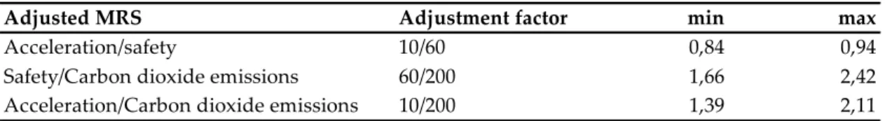
The WTP value only shows the trade‐off between cost and the attribute in question. In order to see the trade‐off between the other attributes, Marginal Rate of Substitution (MRS) is used. The values shown in Table 6 implies that • individuals are willing to give up a little more than 5 % of safety to improve the acceleration with one second; • individuals are willing to emit between 28 and 42 grams more of carbon dioxide to improve acceleration with one second; • individuals are willing to emit between 5 and 8 grams more of carbon dioxide to improve safety with 1 %. Table 6: Values of MRS
MRS (‐X/Y) Safety Carbon dioxide emissions Acceleration
Version 1 Safety 1,00 8,06 ‐0,19 Carbon dioxide emissions 0,12 1,00 0,02 Acceleration ‐5,24 42,23 1,00 Version 2 Safety 1,00 5,52 ‐0,20 Carbon dioxide emissions 0,18 1,00 0,04 Acceleration ‐5,06 27,90 1,00 Version 3 Safety 1,00 6,89 ‐0,18 Carbon dioxide emissions 0,15 1,00 0,03 Acceleration ‐5,65 38,93 1,00