Covered Warrants : How the Implied Volatility Changes Over Time

J

I

B

S

C o v e r e d Wa r r a n ts

How the implied volatility changes over time

Master’s thesis within Finance

Authors: Gustafsson, Lars

Lindberg, Marcus

Tutor: Wramsby, Gunnar

Master’s Thesis in Finance

Title: Warrants

Author: Lars Gustafsson

Marcus Lindberg

Tutor: Gunnar Wramsby

Date: 2005-05-27

Subject terms: Covered Warrant, Finance, Volatility, Implied Volatility

Abstract

Problem: Investors are dependent on the issuers’ valuation of covered warrants because

the issuers also act as market makers. Hence it is crucial that the issuers value each of the five variables used in the Black & Scholes pricing formula in the same way at both the buying and selling occasion. For a covered warrant investor the most important is-sue is the volatility and how it changes over time. This thesis will therefore search for differences in changes of implied volatility between the different issuers.

Purpose: The purpose of this thesis is to analyze differences and similarities between

the issuers’ changes of their covered warrants implied volatility.

Method: The authors have calculated the implied volatility for a sample of warrants

with H&M and Ericsson as underlying assets. Black & Scholes formula has been used and this part of the thesis is made with a quantitative approach. After the implied vola-tility had been calculated correlation tests to the mean as well as to the stock were made. When analyzing the results the authors, in addition to the calculation, used a qualitative method by interviewing market makers. This was made in order to find better explana-tions to the results.

Conclusions: The differences in changes of implied volatility found between different

warrants were small. In general, one warrant changed in the same way as the other ones from one day to another. These results reject the rumors that single issuers adjust their implied volatility in order to make more money. When single events in form of reports were analyzed, the authors found that the issuers changed their volatility in the same way to adjust for the changed uncertainty about the stocks future price. Further, these events clarifies that the basic dynamics of implied volatility is followed by the market. The analysis of how the implied volatility changes with respect to the stock price movements indicates a negative correlation. This implies that an increase in the stock price will lower the implied volatility and vice verse.

Index

1

Background... 1

2

Theoretical framework ... 4

2.1.3 Leverage and elasticity ... 6

2.1.4 Intrinsic value and time value ... 7

2.2 Key ratios of warrants... 8

2.2.1 Delta and Theta ... 9

2.2.2 Vega and Rho... 9

2.3 History of the warrant market ... 4

2.4 Risk ... 10

2.5 Differences and similarities with options... 10

2.6 The Issuers ... 11

2.7 Pricing ... 13

2.8 Black & Scholes option pricing model ... 13

2.8.1 Critique against the Black & Scholes formula ... 13

2.9 Volatility... 15

2.9.1 Future volatility... 15

2.9.2 Historical volatility ... 15

2.9.3 Implied volatility ... 16

2.9.4 The dynamics of implied volatility ... 17

2.10 Previous research ... 18

3

Method ... 20

3.1 The pre study ... 20

3.2 Introduction to the method of the main study ... 21

3.3 Method of choice ... 21

3.4 Sample ... 21

3.4.1 Stocks chosen ... 21

3.4.2 Warrants chosen... 22

3.5 Time of study and measurement intervals... 23

3.6 Black & Scholes ... 23

3.6.1 Implied volatility from Black & Scholes ... 24

3.6.2 Price of covered warrants ... 24

3.6.3 Stock price ... 24 3.6.4 Interest rate ... 24 3.6.5 Dividends ... 25 3.7 Correlation tests ... 25 3.8 Interviews ... 25 3.9 Validity... 26 3.10 Reliability... 27

4

Implied volatility findings... 28

4.1.1 Reports ... 29

4.2 H&M correlation tests ... 30

4.3 H&M warrants correlation to the stock... 32

4.4 Ericsson implied volatility diagrams... 34

4.4.1 Reports ... 36

4.5 Ericsson correlation tests ... 37

4.6 Ericsson warrants correlation to the stock... 38

5

Analysis ... 41

5.1 Question 1... 41

5.1.1 Why the implied volatility becomes zero ... 41

5.1.2 Changes in implied volatility when reports are released ... 42

5.2 Question 2... 42

5.2.1 Negative trend ... 43

6

Conclusions ... 44

7

Reflections and suggestions to further studies ... 45

Figures

Figure 1.1 Turnover of warrants ... 1

Figure 2.1 Time value and intrinsic value ... 8

Figure 2.2 Issuers market shares of turnover ... 12

Figure 2.3 The volatility skew ... 14

Figure 2.4 Average implied volatility surface for SP500 options ... 17

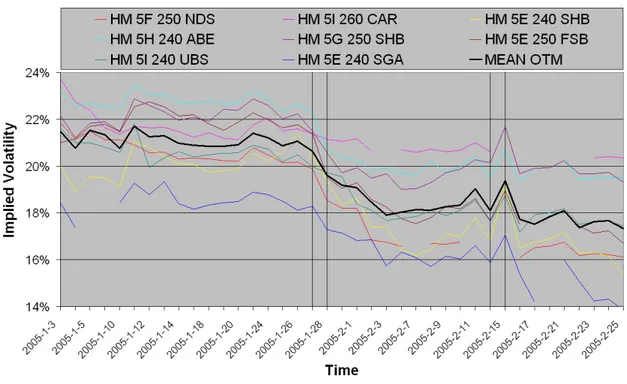
Figure 4.1 Implied Volatility OTM H&M Warrants ... 28

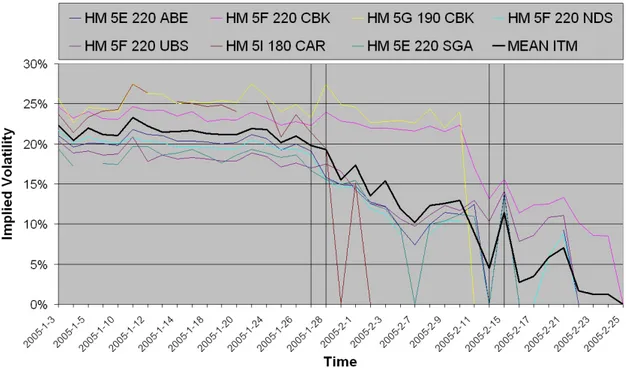
Figure 4.2 Implied Volatility ITM H&M Warrants ... 29

Figure 4.3 H&M warrants correlation to the stock... 34

Figure 4.4 Implied Volatility OTM Ericsson Warrants ... 35

Figure 4.5 Implied Volatility ITM Ericsson Warrants ... 35

Figure 4.6 Ericsson warrants correlation to the stock ... 40

Tables

Table 2.2 Issuers on the Stockholm stock exchange ... 12

Table 3.1 Warrants sample ... 22

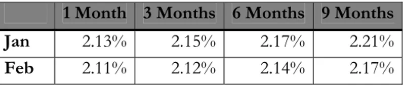
Table 3.2 STIBOR interest rate history ... 24

Table 4.1 H&M reports ... 29

Table 4.2 H&M OTM correlation with mean ... 31

Table 4.3 H&M ITM correlation with mean ... 31

Table 4.4 H&M ITM correlation with mean before Jan. 28th ... 32

Table 4.5 H&M changes in implied volatility due to changes in stock price32 Table 4.6 Ericsson report ... 36

Table 4.7 Ericsson OTM correlation with mean ... 37

Table 4.8 Ericsson ITM correlation with mean ... 37

1 Background

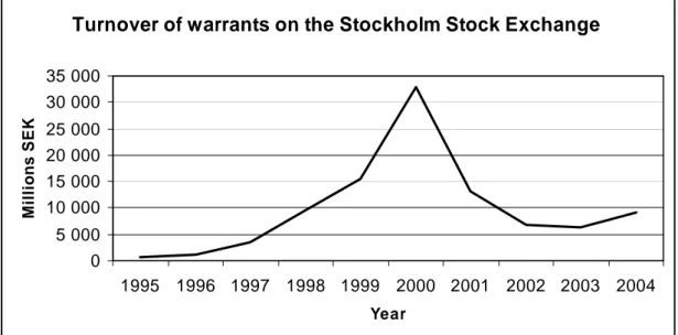
Covered warrants have been traded on the Swedish stock exchange since year 1995. The volume peaked in year 2000 because of the hot market. As one can see in figure 1.1 it was a dramatically drop after the IT- boom year 2000 and the volume for 2004 has not even reached a third of the level in year 2000. What happened the last few years on the Swedish covered warrant market is that the monthly volume has stabilized. In year 2002 the volume was fluctuating from 200 million a month to 1 billion a month. During the following year, 2003, the volume has stabilized and is now between 300 million and 500 million per month (Dagens Industri, 2003).

When the market for covered warrants was falling as heavily as it did during 2001 and 2002 the issuers had to issue new warrants. Because stock prices were declining dramatically the strike price of many call warrants became situated far away from the current stock price. As a result investors were reluctant to trade the outstanding warrants, despite long time to ma-turity. The issuers noticed this and the only way to prevent an even bigger drop in the trade volume was to issue new warrants with lower adjusted exercise prices. To issue new war-rants is far from cheap, in year 2002 the total cost of issuing one new warrant on the Stockholm stock exchange was about 15 000 SEK. The direct cost to the Stockholm stock exchange is about two thirds of the total cost (Huldschiner, 2002).

The cost of issuing new warrants is one aspect that reflects the uncertainty of trading with warrants for the issuers. The problem is that only about one sixth of the issued warrants are actually traded at the market. Consequently the cost of the remaining five warrants, which are rejected by investors, has to be covered by the revenue from the sixth warrant. Therefore it is crucial for the issuer to analyze the demands from the market and satisfy them by issuing attractive warrants (C. Swaretz, personal communication, 2005-03-18).

Turnover of warrants on the Stockholm Stock Exchange

0 5 000 10 000 15 000 20 000 25 000 30 000 35 000 1995 1996 1997 1998 1999 2000 2001 2002 2003 2004 Year Millio n s S E K

Figure 1.1 Turnover of warrants

Derivatives are used by three groups of investors; hedgers, speculators and arbitrageurs. Hedgers use derivatives to hedge their position in the underlying asset. The key aspect for investors hedging is that the cost of, or price received for, the underlying asset is ensured.

of the hedgers. Speculators want to take a position in the market rather than avoid expo-sure to unfavorable movements. Speculators take a position with the fundamental believe that the price will either go up or go down. Using derivatives in this way gives the investor the opportunity to obtain a high profit with a relatively small initial outlay. Arbitrageurs is the third group of investors using derivatives, they are trying to lock in a risk free profit by entering two or more contracts at the same time. These kinds of opportunities are naturally very limited in an efficient market (Hull, 2003).

Covered warrants on the Stockholm stock exchange are commonly used by investors speculating in a future rise in the stock market. About 70-80% of the warrants traded last three years are call warrants which increases in value if the price of underlying asset in-creases. There are although several months when covered put warrants are the most traded ones, often with Ericsson or Nokia as the underlying asset. The covered put warrant is used by investors speculating in a decrease in the underlying asset. The phenomenon that speculators some months prefer covered call warrants before covered put warrants and vice versa implies that speculators tend to base their investment decisions on the mood of the general market (Dagens Industri, 2003).

The main incentive for private investor to invest in covered warrants is that the potential profit is much higher compared to stocks relatively the outlay. This favorable outcome may also be reached in a very short time period. As an unavoidable consequence the risk is also significantly higher than the risk in stocks. An investor can either buy a covered warrant, or sell one that has been purchased earlier. One of the biggest and most important differences between warrants and options is that investors are not allowed to issue warrants but they might be able to issue, take a short position in, options. Regulations and laws are control-ling which actors are authorized to operate as issuers. The result is that the issuer sets the price himself. This means that there will always be buy and sell orders in the market. An-other difference is that the warrant price is lower than an option because the investor will need more than one covered warrant to receive one stock at expiration date (Siljeström, 2001).

1.1 Problem

discussion

The price of a covered warrant is determined in the same way as for an option. Swedish is-suers use the fundamentals of Black & Scholes formula to calculate the value of the rants (C. Swaretz, personal communication, 2005-03-18). To calculate the value of a war-rant with this formula the following variables are used; price on underlying asset, interest rate, time to expiration, exercise price and volatility of the underlying asset (Hull, 2003). There are nine issuers of warrants on the Swedish market. Covered warrants are a profit-able business and hence it is understandprofit-able that all of them are trying to get investors to buy their warrants. The next step for the issuers is to maximize the profit from the trades made by the investors with different methods, e.g. the size of the spread.

Investors are dependent on the issuers’ valuation of the warrants. Hence it is crucial to the investors that the issuers value each of the five variables in the same way at both the buying and selling occasion. When a warrant is priced, expiration day and exercise price are set in advance. The price of the underlying asset is easy to find on the stock market. Interest rate does not have a big impact on the price of a warrant and is used in the same way among the issuers. The value of the volatility used by the issuers on the other hand has a signifi-cant impact on the price. Since this is not a number that can be found in the market it is

natural to suspect that the different issuers value the volatility differently. Implied volatility is simply the volatility that is implied in the covered warrants price.

For a covered warrant investor the most important issue with volatility is how it changes over time. If the implied volatility moves in a, with respect to the market, rational way and the investor sells of the warrants before maturity, the level of the implied volatility does not make a big change for the outcome of the investment. Hence it is useful to know if there are any warrants whose implied volatility does not follow the market movements.

If there are any, what kind of differences are there in the shifts in implied volatility on the same underlying asset between different issuers covered warrants?

If the implied volatility is used differently, on the same warrant, over time the price might change in an unpredictable way. This is a commonly discussed question among investors that trade with covered warrants who think that the issuers are adjusting the volatility to make more money. That would be made by lowering the volatility on a call warrant when the stock increases in value and the other way around for put warrant.

How much does one single covered warrant’s implied volatility change in respect to changes in the underlying stock price?

It is also important that the authors can explain the results from the previous two ques-tions.

Why do the issuers use the implied volatility the way the authors have calculated?

1.2 Purpose

The purpose of this thesis is to analyze differences and similarities between the issuers’ changes of their covered warrants implied volatility.

2 Theoretical

framework

2.1

History of the warrant market

Trading of covered warrants on the Stockholm stock exchange started in year 1995. In the first five years the turn over and closed deals per year steadily increased. The yearly turn-over peaked in year 2000 when it was turn-over 32 billion SEK, which is more than year 1999 and 2001 together. Last year, 2004, the turnover closed at approximately 9 billion after a really strong first six months which was 6 billion. Meaning that during the time July to De-cember 2004 it was a decrease in the turnover for the first time since the dramatically drop in year 2001 and 2002 (Hedensjö, 2004).

In February 2005 a new type of covered warrant was introduced to the market, called turbo warrants. The first issuer was the French bank Société Général and the warrants are listed on NGM’s derivatives exchange market called NDX. The turbo warrants directly hit the top four positions of the chart of the most traded warrants in Sweden. The turnover on NDX increased by 31 million SEK in Marsh after the introduction of the turbo warrants. On the Stockholm stock exchange the turnover for warrants took an opposite direction, it hit a history low 385 Million SEK in March, almost a 50 percent decrease compared to February same year (Huldschiner, 2005).

According to Optionsanalys there are some crucial differences between the historical trad-ing volumes in options, forwards and warrants. They are asktrad-ing the question whether this is how it is supposed to be or just a lack in efficiency on the Stockholm stock exchange. The figures they are referring to is from the first six months during year 2002. Throughout this period the OMX index decreased with devastating 28 percent. The Swedish stock market was now longer in this bubble with hyper active trading and overvaluation which it had been in since year 1999. It was no adjusting to new levels. Despite this tremendous drop in stock prices, the number of closed deals and turnover for warrants the first six months in 2002 was higher than the same period for year 1999 (Optionsanalys, 2002).

The drop in trading with warrants is almost exactly in line with the drop in general stock market trading. The drop from year 2001 to 2002 for trades with stock and interest rate re-lated derivatives is about 7 percent. However, the total premium value from derivatives trading has dropped with over 45 percent for the same period, from 181 million to 100 mil-lion SEK. The thing that makes this interesting is that the drop in the warrant market was 58 percent from the previous year, which can be compared to the total derivatives market drop of 7 percent. The drop in total amount of option contracts and forward contracts was about 6.5 percent while the drop of warrant contract is greater than 50 percent. It is inter-esting why the warrant market more than halved while the options and forwards market just insignificant decreased (Optionsanalys, 2002).

Optionsanalys is giving some explanations to this. First of all they argue that the trade with warrants has been somewhat like a fashion thing for investors. It is something that can generate great outcome fast and easy. The investors do not need any extra knowledge or authorization to be able to trade with warrants, in addition to stocks. A warrant investor is mostly speculating in an increase of the stock market and when the market is in a regres-sion the investor easily loses too much money and abandons the warrant market after some terrible deals (Optionsanalys, 2002).

Investors using options has in general a higher level of knowledge and experience about the market than investors using warrants. To be able to trade with options, investors have to sign a special contract and that makes it more difficult to be an option investor. Option investors are aware of what they are doing and they are alert to the risks but can also see market opportunities by reducing risk for other investments. Option investors are said to use options like the tool it is supposed to be, while warrant investor rather see the warrant derivatives like a lottery ticket (Optionsanalys, 2002).

During the time period 1999 to 2002 about 90 percent of the existing warrants on the Stockholm stock exchange where call warrant. There are several reasons for this, the strongest one is that the warrant market started in the mid nineties and from that point of time to year 2000 the stock market it self had a tremendous increase in value which led to that call warrants being more profitable. The fascinating thing is that after the IT-boom in March 2000 when the stock market started to decrease heavily, warrants investors still in-vested predominantly in call warrants rather that put. This is explained by the fact that war-rant investors rather buy call than put warwar-rants. The results was that instead of purchasing put warrants in a declining market, investors rather waited to find a low position of the market to buy calls (Optionsanalys, 2002).

2.2

Covered Warrants

A warrant is a kind of option that is traded on the stock exchange. When a warrant is bought the right to either buy or sell an underlying asset is actually purchased. This asset is mostly a stock but can also be an index, a basket of stocks, a currency or a commodity. When a warrant is bought a future price as well as exercise price and expiration date is agreed upon. The party that sells the warrant is called an issuer. The issuer is a traditional bank or an investment bank operating on the stock exchange. At the expiration date the is-suer of the warrant is obligated to buy or sell the underlying asset if the buyer wants to ercise the warrant. Because the buyer of a warrant has the right not to participate at the ex-piration date the investor has to pay compensation to the issuer. This compensation is sim-ply the price of the warrant (SG, 2002). In chapter 2.2 and 2.3 SG (2002) will be used al-most exclusively. The authors have decided to use this reference heavily because there is no other publicly known information available about covered warrants characteristics.

2.2.1 Fundamentals of warrants

Parity demonstrates the total number of warrants needed to buy or sell one underlying as-set. The parity must be regarded when several key ratios are calculated; this will be obvious further down in the paper. Therefore it is crucial to understand the parity and what it stands for. Different warrants have different parity. The issuer is using the parity to make the trading more practical for investors. If the parity for a call warrant is 20, the investor needs 20 contracts to be able to buy one share at expiration.

An investor with the fundamental believes that a certain asset will increase in value will buy a call warrant. Vice versa, an investor that speculates in a decrease of an asset will buy a put warrant. These two types of warrants can be compared to call options and put options. If the exercise price of a call warrant is greater than the spot price in the market of the under-lying asset there is no point of exercising the warrant. This is the case because it is then cheaper to buy the underlying asset on the market. Let’s take an Ericsson call warrant as an

the call warrant will logically becomes worthless. On the other hand the price of the under-lying asset might move in a favorable way for the investor and finally exceed the exercise price. This results in that the investor will receive the difference between the exercise price and the spot price.

If the spot price of the underlying asset is below the exercise price of the call warrant, the warrant is out of-the-money. If the spot price is greater than the exercise price the warrant is in-the-money. Vice versa applies for put warrants. For both put and call warrants the fol-lowing is true; if the spot and exercise price is exactly equal to each other the warrant is at-the-money.

2.2.2 Break even

Break-even is a frequently used tool to analyze if a warrant is interesting to invest in. It is calculated when the investor wants to find out the price of the underlying asset which must be achieved if an investment in the warrant will be profitable on the expiration date or not. This example will illustrate this; lets imagine that an investor buys a call warrant in Nokia for 5 SEK with the exercise price 100. In this case one call warrants gives the investor the right to buy one share in Nokia. If the spot price of Nokia rises above 100 SEK he starts to make money but because he paid 5 SEK for the warrant, the underlying spot price must rise to 105 SEK to reach break-even. Break-even for a call warrant is calculated in the fol-lowing way.

Break-even = Exercise price + (parity * price of the warrant)

Considering a put warrant the even is calculated in a slight different way. The break-even price is here showing what price the underlying asset must decrease to before the in-vestment is profitable. That is why the equation for calculating break-even for put warrants looks like following.

Break-even = Exercise price - (parity * price of the warrant)

Premium is the percentage an underlying asset must increase to reach break-even. The premium is a measure which can be compared to the investors believes about how much the underlying asset will increase. If the investor believes that the underlying asset will rise, in percentage terms, more than the premium an investment will take place. The premium is calculated in the same way for both call and put warrants.

Premium = ((Break-even / spot price of underlying asset) -1) * 100

2.2.3 Leverage and elasticity

One of the most important concepts to why investor invests in warrants is an effect called leverage. This tool is used in the way that it gives the warrant a high exposure in the under-lying asset. Exposure in this sense is how much higher return on invested capital the tor will gain compared to investing in the underlying asset. A leverage of 4 gives the inves-tor 4 times higher return per invested SEK. Although mostly invesinves-tors thinks in the way that a leverage on 4 leads to that he or she only needs to invest one fourth of the capital to make the exact same amount of money. The leverage is continuously changing and the formula used to calculate it is illustrated below.

The elasticity is well connected to the leverage; it helps the investor to analyze how sensi-tive a warrant is to price changes in the underlying asset. The elasticity describes how many percent the warrant should change in value if the underlying asset is changing by one per-cent. Leverage multiplied with delta becomes elasticity.

Elasticity = Leverage * Delta

2.2.4 Intrinsic value and time value

The aspect of time is important when investors are considering an investment in warrants. For every day that passes by, the expiration date is getting closer and for every day the un-derlying asset is not moving in the right direction the chance of reaching breakeven is re-duced. The price of a warrant in general has two elements namely, the time value and the real value. Real value is also called the intrinsic value. What is discussed in the rest of this section concerns call warrants.

The intrinsic value is the financial gain that is received if the warrant is exercised. For all time when the price of the underlying asset is below the exercise, meaning when the war-rant is out-of-the-money, the intrinsic value will be zero. The intrinsic value rises linear when the price of the underlying asset increases, no matter how long time it is to expira-tion. At the date of maturity the warrants value will consist of one hundred percent intrin-sic value and zero percent time value (Eiteman, Stonehill & Moffett, 2004).

The second element of the value is the time value. This value only exists because the price of the underlying asset has a potential to move, closer to or further into the money. The time value is supposed to gain or loose the same value if the underlying asset is moving in either direction from the exercise price. This is only a proof of that the warrant price is cal-culated from models with principal based on an expected distribution of possible outcomes around the exercise price. The time value is by far the most discussed and debated one among investors (Eiteman, Stonehill & Moffett, 2004).

Calculating these two different elements might be difficult sometimes. The best way to show it is by illustrating it with graphs and formulas. The intrinsic value is the sum of money the investor would receive if converting his warrants today instead of waiting for the expiration date (Although that is not possible for European warrants). Resulting in the following formula for call warrants;

Intrinsic value = (Spot Price – Exercise Price) / Parity

And the formula for the time value is;

Time value = Price of the warrant – Intrinsic Value

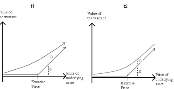
Illustrated in figure 2.1 is what happens if the same warrant is compared at two different occasions. The graph to the right shows what has happened to the time value and intrinsic value e.g. one month after the graph on the left side, all else kept constant. This is called the convexity, or more general “the ice hockey stick”. The grey line, the one that is curved, is the total value of the warrant. The black line, which is straight until it reaches the exercise price and then rises linearly, is the intrinsic value line.

Figure 2.1 Time value and intrinsic value

The two dashed lines in the graphs above shows how big part of the value of the warrant that belongs to the two different elements, time value and intrinsic value. As was discussed earlier in the chapter, the intrinsic value is zero if the spot price is lower than the exercise price. This is illustrated with the two black lines (X) in figure 2.1. After the spot price rises above the exercise price one can se a linear increase in the intrinsic value. If the exercise price of the warrant is higher than then spot price, the time value is one hundred percent of the total value of the warrant. When moving further on in time, from the left to the right graph, the grey line is moving closer to the black line. The reason for this is simply that the closer to maturity, the smaller is the chance that the spot price will increase. Therefore it looks like the shape of an ice hockey stick which is called the convexity principle. X is indi-cating the intrinsic value and the time value is showed by the letter Y. If everything else is kept constant and the only change is that in the right graph the maturity date is closer than it is in the left graph it will result in a decrease in the time value but the intrinsic value re-mains unchanged. The time value will decrease from Y1 to Y2. However, the right graph is showing that a warrant still has a value even if it is far out-of-the-money and close to ma-turity .

2.3

Key ratios of warrants

To be able to measure and analyze the potential future movement of a warrant there are some key features that are used more frequently than others. These different ratios are all deduced from the Black & Scholes formula and they are called the Greeks. The primary reason for using these different key ratios is to measure the characteristics of the warrant. However, investors are also using them to neutralize and reduce the risk in their portfolios. This can for example be done by delta hedging, gamma hedging or theta hedging. The au-thors will not go further into these different hedging techniques since they are not relevant for the thesis. It is crucial to understand that all the key ratios described and calculated in this chapter are only valid if all other factors are constant and not changed. Therefore one must be careful when using the different ratios for calculations and analysis.

2.3.1 Delta and Theta

Delta measures how many SEK the price of one warrant position will change if the price of the underlying asset increases by one SEK at a specific time. Delta is always between 0 and 1 when it is calculated for a call warrant. The highest delta will be when the warrant is in-the-money. An example could be a call warrant of Nokia with parity of 1 and a delta of 0.70. If the share of Nokia increases by 10 SEK the price of the warrant will increase with 7 SEK. This means that a warrant with a delta of 0 will not move at all if the underlying asset is increasing and a warrant with a delta of 1 is moving exactly as much as the underlying as-set in absolute terms. A rule of thumb is that delta is 0.5 if the warrant is at-the-money. Delta can also be seen as the probability that the warrant will have a real value at the expi-ration date. If the price of the underlying asset is far greater than the exercise price, the warrant will probable be in-the-money at the expiration date. Therefore the delta of a war-rant like this one should be very high, almost 1. Another variable affecting the delta value is the time to expiration. When the expiration date is approaching the shape of the delta curve will become steeper because a shift in the price of the underlying asset can be of cru-cial importance of having an in-the-money warrant or not.

Theta value measures how fast the time value is decreasing when the warrant is getting closer to expiration. Mathematically the theta value can be described as the derivative of the price of the warrant consideration the time left to expiration. Theta indicates how much of the time value that is lost in one trading day if every thing is else is constant. If a warrant is priced at 15 SEK and has a theta value of 0.5, the price of the warrant will be 14.5 the next coming trading day. The theta value is increasing with and accelerating force every day: The closer the warrant comes to it expiration, the higher theta if everything else is constant.

2.3.2 Vega and Rho

Until now the volatility has been assumed to be constant. In practice it is not that simple, the volatility changes over time. This means that the value of the warrant is not only af-fected by delta and theta value but also the vega value. The vega of a warrant is the rate of value change with respect to the volatility of the underlying asset. If for example the vega value is high it means that the price of the warrant is very sensitive to changes in the vola-tility of the underlying asset. If an investor has a position in the underlying asset the vega value is zero. If the investor has a portfolio with zero in vega value, it will probably mean that the gamma value will be high. However, it is possible to have a portfolio of both vega and gamma values equal to zero but then at least two different warrants on the underlying asset must be used. Calculating the vega value from the Black & Scholes model can be con-sidered wrong because the underlying assumptions from the model is that the volatility is constant. It would be preferred to calculate the vega values from models and formulas which assumes that the volatility is stochastic. However, calculations have been made from both types of models and the result is that there is a very small difference (Hull, 2003). The rho of a warrant is how much the price of warrant changes if the interest rate changes. If a warrant has a rho value of 0.40 it means that if the risk-free rate changes from 8% to 9% the price of the warrant will change 0.004 (Hull, 2003). This is a very small change and the value of warrants is not affected by interest rate very much.

2.4 Risk

Both the investor and the issuer are exposed to risks. Variables that can affect the price in an unfavourable direction, and therefore is considered as risks are; price of underlying as-set, the interest rate and the volatility. The issuer of the warrant is using a highly sophisti-cated way to reduce the risk. Different positions demands different ways of hedging, this means that the issuer constantly have to be alert and carefully listen to the market at all time. The issuers are not trying to gain from the warrant trading by taking a high risk, they are actually hedging every deal made. Usually it leads to lower profit but with significant lower risk. An advantage the issuers have is that they are relative big on the market and can therefore lower their costs of hedging. The private investor on the other hand does not have the same possibility of hedging the taken position (Siljeström, 2001).

Investors that are seeking positions in warrants or options are mostly not interested in hedging the warrant position. Because it might be the intention to take a high risk and reach a possible high return. The most interesting variable for the investor is the risk of the price of the underlying asset in the meaning that he can not hedge the interest rate or the volatility risk. To make an attempt to calculate the risk of trading with warrant there is something called the Value at Risk (VaR). VaR tries to measure the total risk of investing in a warrant. VaR is using two parameters, the time horizon and the confidence level. After calculating the VaR the investor should be able to make the following statement; “We are X percent certain that we will not lose more than V dollars in the next N days”. VaR is commonly used by both investors and banks because it is easy to understand and it ends up in asking the question “How bad can things get?” An investor that is willing to take a higher risk is also willing to accept a higher VaR (Hull, 2003).

When investors sit down together to discuss their last trades it is highly uncommon that they talk about their disasters. Instead they talk loudly about all their successes and perhaps sometimes about a disaster some other broker made. This is just being human and what separates a successful trader from an unsuccessful one is the skill to survive the disasters. A trader using a spread with a large margin for errors and a good theoretical edge is probably one of the successful ones. Even if this kind of trader is losing money it will not be that much as if a spread with a small error margin would have been use. It is impossible to take into account all the different risk factors and measurement such as delta, gamma, vega, theta and so forth. Doing this would only end up in trades with almost none theoretical edge and very high transactions costs. One thing to keep in mind is that a well diversified portfolio is not always the one that shows the greatest potential profit when things go well. It is the one which shows the least loss when things go really bad. Remembering that the risk which is combined to the loss scenario is the most important ones (Natenberg, 1994).

2.5

Differences and similarities with options

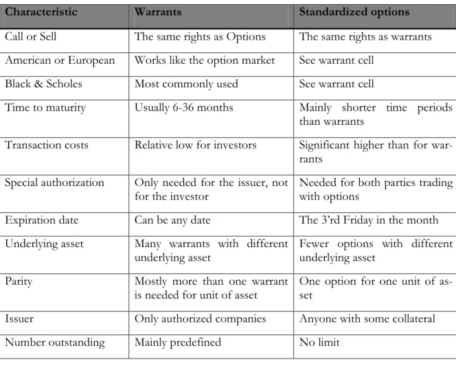
Warrants are like options, but options are not like warrants. This implies that warrants have the same characteristics as standardized options and some additional ones, which options do not have. The differences and similarities are here shown in table 2.1 below (Blomgren & Olsson, 2003).

Table 2.1 Differences and similarities between warrants and options

Characteristic Warrants Standardized options

Call or Sell The same rights as Options The same rights as warrants American or European Works like the option market See warrant cell

Black & Scholes Most commonly used See warrant cell

Time to maturity Usually 6-36 months Mainly shorter time periods than warrants

Transaction costs Relative low for investors Significant higher than for war-rants

Special authorization Only needed for the issuer, not

for the investor Needed for both parties trading with options Expiration date Can be any date The 3’rd Friday in the month Underlying asset Many warrants with different

underlying asset Fewer options with different underlying asset

Parity Mostly more than one warrant

is needed for unit of asset One option for one unit of as-set Issuer Only authorized companies Anyone with some collateral Number outstanding Mainly predefined No limit

2.6 The

Issuers

On the Swedish warrant market the issuer and the market maker is the same institution. Even if it is two different roles with different missions they are highly correlated on the warrant market. The issuer is the one that issues the warrant from the beginning. It is the issuer that determines the underlying asset, the parity, the exercise price and the expiration date. The role of the issuer is to launch new warrants and make sure that the warrants are what the market is demanding. When the market starts to trade the warrant the issuer be-comes the market maker. The market maker guarantees liquidity in the market and make sure there are both sell and buy orders on the market. It can be said that the market maker is working for the issuer. The market maker is also responsible for the system updates and that everything is working smooth and without any interrupts (Blomgren & Olsson, 2003). As one can see in figure 2.2 Svenska Handelsbanken was the market leader during year 2004 with a market share of 40.8%. Handelsbanken has a good relationship to its custom-ers and shows a really great commitment to what they are doing. We have a very good in-vestor relationship which is combined with good information brochures and prospects about our warrants for the investors, says Peter Frösell (P. Frösell, personal communica-tion, 2005-03-16).

SHB 40,8% UBS 33,1% FSB 3,6% CAR 2,9% SG 11,0% CBK 5,6% ABE 1,2% NDS 0,4% SEB 1,4%

Figure 2.2 Issuers market shares of turnover

The warrants names might look a little complicated for the first time trader, even though the names are build in a very structured way, namely in the following:

Example: HM 5H 240 ABE

HM= Underlying stock, Hennes & Mauritz

5H= Expiration date, august in year 2005 (A= January, B=February, C= March and etc.) 240= Exercise price, 240 SEK in this example

ABE= Issuer, in this case Alfred Berg

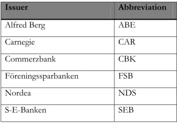
Table 2.2 below shows all the abbreviations for the issuers on the Stockholm stock ex-change.

Table 2.2 Issuers on the Stockholm stock exchange

Issuer Abbreviation

Alfred Berg ABE

Carnegie CAR Commerzbank CBK Föreningssparbanken FSB

Nordea NDS S-E-Banken SEB

Société Générale Acceptance SGA Svenska Handelsbanken SHB

UBS Warburg UBS

2.7 Pricing

There are several ways to price an option. The one that is most used is the Black & Scholes formula from 1973. Nowadays it is very common to use some kind of modified version of the Black & Scholes formula to correct for some errors. (Hull, 2003)

One other kind of pricing technique is to price with binominal trees. This I made by divid-ing an options life time in to small periods where the stock can only move in to two possi-ble values. By creating trees with numerous calculations an option value can be calculated.

2.8

Black & Scholes option pricing model

Black & Scholes options pricing formula was made in 1973 with the basic assumption that the price of the option was at such level that there was no arbitrary opportunities. By this is meant that one could not make sure profits by creating a portfolio with long and short po-sitions in the option and underlying asset. Before Black & Scholes created there formula there had been a number of attempts to make a good formula but they all made arbitrage opportunities possible (Black & Scholes, 1973).

The mechanics of an option is simple; if the price of the underlying asset increases the value of the options increases (call option). If there is more time left to maturity the option is worth more and if the underlying asset is more volatile the option has a higher price. The dynamics of the formula implies that a 1 % change in the underlying asset makes a more than 1 % change in the option (Black & Scholes, 1973)

There are five assumptions that Black & Scholes (1973) stated in order to make the for-mula accurate:

1. The variance of the rate of return is constant over the life of the option and known by the market participants.

2. The short term interest rate is known and constant over time.

3. The option holder is protected against distributions that affect the price of the op-tion.

4. Over a finite interval the returns on the stock are log normally distributed. 5. There are no transaction cost, no limitations on short selling.

2.8.1 Critique against the Black & Scholes formula

One commonly known inaccuracy with the Black & Scholes formula is the volatility skew. This is shown in figure 2.3 below. The higher strike price of an option the lower is the

im-plied volatility. Traders use this skew to price equity option. The skew is not the same for all underlying assets (Hull, 2003).

Implied volatility

Strike Price Figure 2.3 The volatility skew

There are several possible reasons why the skew occurs. One of these concerns leverage. As a company’s equity value declines, the leverage increases. This results in a higher volatil-ity in the equvolatil-ity which in turn makes even lower stock prices likely. (Hull, 2003)

Another interesting fact is that before the stock market crash of in October 1987, this skew in volatility did not exist. Hence there has been suggestions that this skew is something that can be called crashofobia. There is also a tendency that whenever the market declines the skew gets less pronounced, and the other way around. (Hull, 2003)

2.8.1.1 Macbeth & Merville 1979

Macbeth & Merville (1979) tested Black & Scholes formula in a big research that included six underlying stock and all their call options during one year. They came to the conclusion that the formula predicted the price of the options wrong in three ways. First the formula gave lower than market price for in the money options and higher than market price for out of the money options. Second, the phenomenon described seems to be greater if the option is further out or in the money. Third, out of the money options are lower valued on the market when there is a short time to expiration (less than 90 days) than Black & Scho-les formula values. (Macbeth, 1979)

2.8.1.2 Manaster 1980

Manaster discusses Macbeth & Mervilles research and says that other models can predict the option price just as good as the Black & Scholes (1973) model. (Manaster, 1980)

2.8.1.3 Rubinstein (1985)

Rubinstein made a very big research where he tested alternative pricing models against Black & Scholes (1973) model. The result shows that there are none of the models in the study that predicts the option price better (Rubinstein, 1985).

2.8.1.4 Bakshi

In this research the author concluded that there are an extreme amount of different models that are based on the Black & Scholes 1973 formula. Some of these new formulas include variables that make them more precise, and the authors themselves have also made yet an-other model. According to them there are ways to improve Black & Scholes, but there are so many formulas out on the market that there is a great difficulty in choosing one. That is the reason that they have made a formula that is somewhat concluding many of the previ-ous formulas. (Bakshi, 1997)

2.9 Volatility

Traders of an instruments as well as options are interested in the direction of the market. The difference between these two is that the option trader is extremely sensitive to the speed in which the market moves. If the market moves in a slower speed the chance that an underlying asset is to break through the exercise price of an option is less likely. Market speed is volatility. (Natenberg, 1994)

The volatility of a stock measures the uncertainty about the returns provided by the stock. With the stock price as the mean the volatility is the standard deviation. (Hull, 2003)

For example a stock is traded at SEK 100 and the yearly volatility is 20%. This volatility represents the price change, one year from now, within one standard deviation. One ex-pects the stock to be traded somewhere between SEK 80 and SEK 120 approximately 68% (one standard deviation) of the time and between 60 and 140, 95% (two standard devia-tions) of the time.

2.9.1 Future volatility

The future volatility describes the future distribution of the price of an underlying asset. This is the actual number that is referred to when volatility is put in to option pricing mod-els. To know the future volatility is to know the odds. That is if one know the volatility and uses that value in a pricing model, the accurate theoretical option value can be calculated. If one can do that he or she can be certain of long run profits of their trades (Natenberg, 1994).

2.9.2 Historical volatility

Even though no one knows the future it is important for an investor to in some way pre-dict how much the market is going to move. This is more important to an option investor than to a stock trader, because volatility is a big part of the value of an option. One of the easiest ways to predict the future is to see to the past. If the asset has had volatility between 10% and 20% over the last years, the chance of the asset having a volatility of 5% or 30% is not very likely. It is important to point out that it is possible, but not likely for the asset to move in an unpredicted way (Natenberg, 1994).

There are a number of ways to calculate historical volatility but there are two variables that is included in all these models. First is the time limit of how far back one wants to look. It can be any time period; one week, one year, five years etc. The other variable is how often one wants to collect the data about the price of the asset. For one week it might be

interest-high. As mentioned this is an extreme case, volatility of an asset seems to be about the same whether one looks at one day, week or month (Natenberg, 1994).

2.9.3 Implied volatility

Previous discussions about volatility (future, historical) have been about the volatility of the underlying asset. The volatility that is implied in an options price is simply called implied volatility. To clarify how the implied volatility works an example will be provided (Naten-berg, 1994);

A Stock is traded at SEK 90 and you value the volatility to 20 % for the coming three months (The numbers of this example is not correct, they are just guidelines). Hence you calculate the value of a call option with expiration in three months and with an exercise price of SEK 92 to SEK 2/Share with Black & Scholes formula. When you look at the marketplace it is traded at SEK 2.50 per share. Why are these two values then different? If one looks at the values that were put in to Black & Scholes one by one it is easier to see which one or ones that are different. First of is the exercise price, which obviously is the same. The time to expirations is also the same as well as the interest rate and price of the underlying asset. The one and only variable that is different between the two values is the implied volatility.

Implied volatility of an option cannot be analytically calculated because of the structure of Black & Scholes formula. To get the implied volatility one has to make iterations of the formula with the other know variables. The implied volatility in the example above with the market price of the call option is then 23%. So the marketplace implied volatility is higher than the calculated one. If one believes that the implied volatility is below 22% the option would not be purchased and if one believes that it is above that level the option would be purchased (Natenberg, 1994).

Even though the option premium is the price of an option it is often referred to as implied volatility. Implied volatility determines the relative value of an option. If a forecast of vola-tility is done with respect to the past and that it shows that it is low, one can say that the option is undervalued and that it would be good timing to buy it. A trader can also com-pare implied volatility on different options that are somewhat similar, to find out if any of them are priced relatively high or low (Natenberg, 1994).

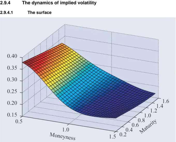
2.9.4 The dynamics of implied volatility

2.9.4.1 The surface

Figure 2.4 Average implied volatility surface for SP500 options (Cont & Fonseca, 2002)

Figure 2.4 show the term structure of implied volatility. The underlying asset the implied volatility is calculated on is SP500 index. Moneyness is exercise price divided by spot price and show how far in or out of the money the option is (1 is at the money). The surface is commonly known, where moneyness is the most affecting variable and time to maturity changes the implied volatility by a small amount. As one can see, the implied volatility is relatively very low when the option is in the money and high when it is out of the money (Cont & Fonseca, 2002).

2.9.4.2 Report or news

One basic way to value the volatility, used to price warrants, is to look at the past volatility of the underlying asset. This can be done by, either taking an average of the past, or by weighting each time period in the past differently. The second method can be made in many ways with a number of different weights. Two commonly used models are called ARCH and GARCH (Natenberg, 1994)

The problem is that looking at the past is not enough. The implied volatility measures the uncertainty on the market. Hence, when an annual report for the company or a govern-ment spending report is about to be released the uncertainty may be high. When the date of the news is know, and the news possible will have a big impact on the stock price (or

been released the uncertainty is gone and therefore the implied volatility is decreased. What this does to an option trader is that the premium of the option increases before a report and then decreases somewhat afterwards (All other variables held constant). Sometimes this implied volatility difference is so big that, even if the report turns out to good and the stock price increases, the option price will decrease (call option). A report can also create uncertainty if a company for example has had a stable period and the report shows on fu-ture turbulence (Natenberg, 1994).

2.10 Previous

research

In 1998 Dumas, Fleming and Whaley wrote an article in Journal of Finance about a subject discussed by many authors before them. The subject is volatility; more specific this article is about the hypothesis that asset return volatility is a deterministic function of asset price and time. Dumas et al. used a deterministic volatility function (DVF) option valuation model. The potential of the DVF is that it can fit the observed cross section of options prices ex-actly. The authors used S&P 500 options from June 1988 to December 1993. The main purpose of the paper was to examine the predictive and hedging performance of the DVF option valuation model. The Black & Scholes model from 1973 is also taken into consid-eration, while trying to explain the implied volatilities across all the exercise prices and dif-ferent times to maturity. The expected future volatility is a major part in the finance theory and is also reflected in this paper by Dumas et al. The future volatility is very often fore-casted and market analysis is depending on past volatility in their forecast. Dumas et al. come up with some vital conclusions, for the first they conclude that their calculations proves that parsimonious model works best in samples like theirs. For the second they ar-gue that when DVF models used one week after to calculate the prediction errors grow lar-ger as the volatility becomes thrifty. For the third, and last, Dumas et al. writes that hedge ratios calculated by the Black & Scholes formula are better than hedge ratios obtained from the DVF option value models (Dumas et al., 1998).

Hull and White (1987) wrote an article on the problem with European call options on stocks with stochastic volatility on the underlying asset. This was an unsolved problem and the authors where the first two professors to examine the discussed problem. The method used was to calculate series with stochastic volatility on options which were uncorrelated with the underlying security price. It is shown for such a security that the Black & Scholes formula overvalues at-the-money options and undervalues deep in and at-the-money op-tions. The range over which this can be said to be true for overpricing is within 10 percent of the exercise price. The error calculated can be as big as 5 percent. The result from this study can be directly transferable to put options through the use of put-call parity. It is also possible to transferable the result to American calls if they have a non dividend paying stock as a underlying asset. American puts on the other can not easily be applied with the result from this research (Hull & White, 1987).

Huang and Chen (2002) used the model invented by Hull and White 1987 (HW) to make new research on samples not taken into consideration by Hull and White. Huang and Chen’s study from 2002 investigates the stochastic volatility option pricing HW model with the main focus on covered warrants traded on the Taiwan Stock Exchange (TSE). Warrant values from HW’s model and those values from the Black & Scholes model are compared with new observed option premiums. The study also take into consideration time to matur-ity, volatility and the risk-free rate; to be able to measure the pricing biases related to the warrant strike price. Result from Huang and Chen’s research shows that the HW model with implied volatility outperforms others in predicting the warrant prices. This indicates

that pricing models incorporated with stochastic volatility feature can improve the pricing of warrants. Huang and Chen furthermore make the conclusion that models with implied volatility outperform models using other types of time-series volatility. The models tend to underprice covered warrants, at least the one traded on the Taiwan Stock Exchange. The results error is systematical related to the degree to which the warrants are in-the-money, and the volatility of the underlying assets of the warrants (Huang & Chen, 2002).

According to Blomgren and Olsson (2003) warrants with low probability of being in-the-money at the expiration date has a lower risk adjusted return than warrants with a higher chance of being in-the-money. The authors made a research on the return of warrants dur-ing the time period 1998 to 2003. The study included both call and sell warrants on Erics-son and Nokia on the Stockholm Stock Exchange. The method used was that all the avail-able warrants on the two underlying asset where bought the first trading day each month and then sold the first trading day in the next coming month. All the warrants where then divided into groups after what probability they had of being in-the-money at the expiration date. Each group consisted of interval of 10 percent. Blomgren and Olsson (2003) finally calculated the return on each group of warrants with consideration to the return of the un-derlying stock and the changes in the elasticity. For call warrants the group with 0 to 10 percent probability had a substantial lower return than the other groups. For put warrants the two lowest group of probability, group 0 to 10 percent and group 10 to 20 percent, had significant lower return than the rest. Analyzing the result the authors come up with two causes, the implied volatility and the spread, both contributing to that the result looks like they do.

In 2004 Lindbom, Persson and Ramström made a similar study to the one above. The pur-pose of their thesis was to estimate the expected return on warrants and compare it to some alternative investments. Their study included a Monte Carlo simulation made on three stocks on the Stockholm Stock exchange. Lindbom et al. (2004) calculated the ex-pected return on 42 different warrants and came up with the astonishing result that war-rants had a negative expected return of about 26 percent. In addition to that, the authors discovered differences between different issuers as well as different types of warrants. As-tounding to the authors was that a low premium together with a high parity seemed to have negative effect on the expected return.

Kristoffersson (2002) made a research on the derivatives market. The purpose was to test whether the most popular option pricing models provides accurate result or not and to de-scribe different strategies that can be used regardless what kind of market the investor is active in. The value calculated from Black & Scholes- binominal and trinomial tests was compared to the true market value on different options on Ericsson and Nokia. The lack in each model is determined by the author, examining if the differences between the fair cal-culated value and the market value was significant or not. Kristoffersson provided the re-sult that difference in values on Nokia options where not big at all. However, the differ-ences on the Ericsson options where quite big and the fair value separated from the market value. Explanation to this may be that the volatility estimations are too high. Finally can be said that the three different models provides very similar results and all of them tends to provide better results on call rather than on put options (Kristoffersson, 2002).

3 Method

Bell (2000) argues that the initial step in the process of writing a thesis is to formulate the purpose. The purpose should be well connected to the problem stated by the authors. When this is done the authors’ focus falls on the theories concerning the subject. The choice of method used to solve the problem and fulfill the purpose is determined by the outline of the problem and the purpose.

The two major elements of traditional science methods is positivism and hermeneutic. The main argument for positivism is the confidence in scientific rationality. According to posi-tivism the knowledge and fact in a survey should be possible to measure in an empirical way. All estimations and guesses should be replaced by real measurements to receive a bet-ter result. Validity and reliability are two tools used to follow positivism. Criticism against positivism is that the human being itself is an object and the method excludes feelings, ex-periences and valuations. Using the positivism method prevents the authors from gaining a helicopter perspective of the whole picture (Wallén, 1996).

Hermeneutic on the other hand uses different symbols and feelings in empirical gathering to find a result. Authors using the hermeneutic method are analyzing both part by part and the whole perspective at the same time; they are even examining different antagonisms within the whole perspective (Wallén, 1996). Lundahl and Skärvad (1992) criticize the her-meneutic method because it can not separate facts from valuations, in other words objec-tivism and subjecobjec-tivism. Further on they argue that it is hard to be impartial using a herme-neutic method. Using this kind of method assumes that the authors already have knowl-edge and personal experience in the field.

This thesis will have scientific weight on the positivism method because the result from the tests has a high objectivism. The pre study which was conducted through interviews with issuers and the part where the authors asked for comments from involved parties are both examples which can be argued to be hermeneutic.

Quantitative and qualitative are two different research methods applicable in a scientific study. In a quantitative study the measuring is vital. Studied units will receive a value for a specific variable and the purpose is to see a picture of all units (Jarlbro, 2000). This study has variables that need to be measured by numbers and displayed by figures and tables. Therefore this part of the study is quantitative.

In contrast to quantitative, a qualitative study works with ideas rather than units. When one searches for ideas instead of units, one does not know what the ideas are until they are found (Jarlbro, 2000). The purpose of this thesis is to explain differences and similarities between the issuers’ changes of their covered warrants implied volatility, therefore it is naturally to adopt a qualitative approach after the quantitative one. This is because the au-thors then can explain the results in the best way possible.

3.1 The

pre

study

Before the main study took place a pre study was made. It was made because the authors needed to know more about the issuers work. The pre study was made by interviewing three of the issuers on the Swedish market; Föreningssparbanken, Handelsbanken and UBS Warburg. These were the ones that were willing to do interviews. With the information gathered from these interviews the problem could be stated and the questions could be

formulated. There is not much emphasis on the pre study in the thesis since it was made to get a more precise research from the beginning.

3.2

Introduction to the method of the main study

The method is divided in two parts. The first part is quantitative, where the authors com-pared the implied volatility between the different issuers over time. When these calculations were completed, the second part of the investigation took place. That was to explain the re-sults from the quantitative research in different ways, e.g. by discussing the rere-sults with the issuers.

3.3 Method

of

choice

In order to solve the questions stated, a quantitative study has been carried out. By calculat-ing the implied volatility over a time period for each of the issuers on the Swedish market, the authors could see if there were any differences in the changes of volatility between them. Implied volatility has been calculated using Black & Scholes option pricing formula. Data from the calculations are mostly presented in two sub groups under each of the two stocks. The sub groups are “in the money” warrants and “out of the money” warrants. By calculating the mean for each of these sub groups it was possible to see just how far each and one of the covered warrants were from the mean in its own sub group. The warrants were divided in these two groups because the warrants implied volatility differs greatly de-pending on if they are in or out of the money.

With these numbers known, a qualitative study was performed in order to get an under-standing of why some of the issuers changed their implied volatility differently from the others. It can depend of different pricing techniques or policies etc. That is what the inter-views with the issuers are supposed to explain.

3.4 Sample

There are covered warrants on many different types of underlying assets; stocks, gold, oil, currency etc. In this thesis their will only be covered warrants included that has a stock as an underlying asset. The authors made this decision because these are the ones that are most traded. Because of that there are a greater number of them issued on the market. This makes it possible to compare the issuers with somewhat similarly warrants (Stockholms-börsen, 2005).

The study included a comparison between the different issuers implied volatility on their covered warrants. Because of that the selection obviously had to include at least one cov-ered warrant from each issuer. In order to get more precise results from the study the au-thors chose to include covered warrants on two stocks. The auau-thors also chose to include two warrants from each issuer per stock.

These are the basic setup of the selection. More about the exact covered warrants included will follow in 3.4.2.

warrants with Ericsson, Nokia, H&M, Skandia, and Tele2 as underlying asset were the most traded ones. The data limited the research to these stocks and since Ericsson was the biggest that was the first stock chosen. Number two was randomly chosen from the re-maining four and turned out to be H&M. Warrants with the following underlying assets were chosen;

• Ericsson B • H&M B

3.4.2 Warrants chosen

In order to exclude errors that could be present in single warrants, two covered warrants were chosen from each of the issuers. By doing this the warrants could be compared from each issuer to check for possible errors. Because of the volatility skew that is described in chapter 2.8.1 the authors chose to select covered warrants that had an exercise price close to the spot price, at least at the first day of the research. The selection was made like this;

1. A warrant that had an exercise price under, but close to the exercise price was cho-sen

2. A warrant that had an exercise price over, but close to the exercise price was cho-sen

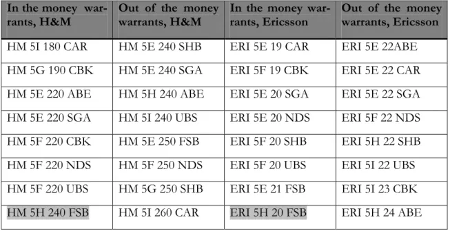
The chosen warrants is displayed in table 3.1 below, they are arranged by their exercise price.

Table 3.1 Warrants sample

In the money

war-rants, H&M Out of the money warrants, H&M In the money war-rants, Ericsson Out of the money warrants, Ericsson

HM 5I 180 CAR HM 5E 240 SHB ERI 5E 19 CAR ERI 5E 22ABE HM 5G 190 CBK HM 5E 240 SGA ERI 5F 19 CBK ERI 5E 22 CAR HM 5E 220 ABE HM 5H 240 ABE ERI 5E 20 SGA ERI 5E 22 SGA HM 5E 220 SGA HM 5I 240 UBS ERI 5E 20 NDS ERI 5F 22 NDS HM 5F 220 CBK HM 5E 250 FSB ERI 5F 20 SHB ERI 5H 22 SHB HM 5F 220 NDS HM 5F 250 NDS ERI 5F 20 UBS ERI 5I 22 UBS HM 5F 220 UBS HM 5G 250 SHB ERI 5E 21 FSB ERI 5I 23 CBK HM 5H 240 FSB HM 5I 260 CAR ERI 5H 20 FSB ERI 5H 24 ABE

Note that two of FSBs warrants were issued the last of January and therefore only had data for less than half of the period; for that reason the authors chose to exclude them (shaded in table 3.1).

The covered warrants were diveded into these subgroups because of large differences be-tween in the money and out of the money warrants implied volatility. When the implied volatilities then were compared, a better mean for each group could be used.

Covered warrant that had a price below SEK 0.1 was excluded and if it was possible, the ones that had prices below 0.2 were also excluded. This because the large changes in the warrant price at each level e.g. the smallest possible change for a SEK 0.05 warrant is 20%.

3.5

Time of study and measurement intervals

The length in time of the covered warrant observations was two months, January and Feb-ruary of 2005. The authors’ restricted time made a limitation to the number of observation that could be made, therefore two months were chosen. In order to get a period of time where some new information was released that affected the implied volatility, the time of the annual business reports for the two companies were chosen.

January and February of 2005 includes 39 days when the stock exchange was open. To get an accurate implied volatility daily observations had to be made. That is 39 days, 2 stocks, 8 issuers with 2 covered warrants on each (FSB only had one warrant for each stock). All this sums up to about 1100 observations of implied volatilities on just the warrants.

3.6

Black & Scholes

To calculate the implied volatility of the covered warrants that were chosen, an option pric-ing formula had to be used. In order to get as precise results as possible, the best formula to be used was the same as the issuers. The authors found that Black & Scholes option pricing formula were used by the Swedish issuers. Even though the formula had been modified to fit the needs of the issuer, the core concept of it was the same through out the market (P. Frösell, personal communication, 2005-03-16).

The way to calculate the implied volatility was then clear; the Black & Scholes formula. ) ( ) ( _{1 2} 0N d Ke N d S c= − −rT T T r K S d σ σ /2) ( ) / ln( 2 0 1 + + = T d T T r K S d σ σ σ − = − + = 1 2 0 2 ) 2 / ( ) / ln( maturity to Time T Volatility erest Riskfree r price Exercise K price Stock S price Call c = = = = = = σ int 0