View of Directional Dependence in the Analysis of Single Subjects

2016, 2(1–2)

Published by the Scandinavian Society for Person-Oriented Research Freely available at

http://www.person-research.org

DOI: 10.17505_{/jpor.2016.04}

Directional Dependence in the Analysis of Single Subjects

Wolfgang Wiedermann

1

_{, Alexander von Eye}

2

1_{University of Missouri, Columbia} 2_{Michigan State University}

Contact

wiedermannw@missouri.edu

How to cite this article

Wiedermann, W. & von Eye, A. (2016). Directional Dependence in the Analysis of Single Subjects. Journal of Person-Oriented Research, 2(1–2), 20–33. DOI: 10.17505/jpor.2016.04

Abstract: Many statistical methods applied in person-oriented research make use of theoretical principles originally derived in a oriented context. From this perspective, it naturally follows that advances originated in variable-oriented methodology may potentially contribute to the development of methods suitable for person-variable-oriented perspectives. Direction Dependence Analysis (DDA) constitutes one of these recent advances and provides a framework to statistically evaluate asymmetric properties of observed variable relations. These asymmetric properties enable researchers to make statements whether a model of the form x→ y or a model assuming y → x is more likely to approximate the underlying data-generating process in non-experimental settings. The present article introduces DDA to the context of person-oriented research and extends the DDA principle to (linear) vector autoregressive models (VAR) which can be used to describe individual development. We show that DDA can be used to empirically evaluate directional theories of (potentially multivariate) intraindividual development (e.g., which of two longitudinally observed variables is more likely to be the explanatory variable and which one is more likely to reflect the outcome). An illustrative example is provided from a study on the development of experienced mood and alcohol consumption behavior. It is demonstrated that VAR-DDA resolves the issue of identifying the direction of contemporaneous effects in longitudinal data. Temporality issues of directional theories used to explain intraindividual development, guidelines to achieve acceptable power, methodological requirements, and potential further extensions of DDA for person-oriented research are discussed.

Keywords: Direction dependence, vector autoregressive model, single-subject data, intensive longitudinal data, non-normality

Introduction

The person-oriented approach – deeply rooted in the holistic-interactionistic research paradigm (see, e.g., Mag-nusson, 2001) – emphasizes the individual as a function-ing entity and focuses on individual characteristics of per-sons, their dynamic development over time, and their vari-ation across contexts. Modern conceptualizvari-ations of the person-oriented approach can be summarized by seven tenets which acknowledge 1) individual specificity of de-velopment, 2) process complexity, 3) interindividual differ-ences in intraindividual change, 4) the characterization of processes in terms of patterns, 5) holism, 6) pattern

parsi-mony, and 7) dimensional identity (cf.Bergman & Magnus-son,1997;Bergman, Magnusson, & El Khouri,2003;von Eye & Bergman,2003;von Eye, Bergman, & Hsieh,2015). This person-oriented perspective is opposed to a variable-oriented approach which focuses on variation of charac-teristics across individuals to establish statements about the correlational structure of variables, their constancy and change over time, and systematic differences across con-texts on a population level.

Various statistical methods have been identified as be-ing well-suited to study person-oriented research questions (cf. Bergman & Magnusson,1997;Sterba & Bauer,2010; von Eye et al.,2015). These include (among others)

cross-sectional mixture models, latent growth mixture models, item response theory models, configural frequency and log-linear models, hierarchical linear models, and meth-ods for the analysis of single subjects (such as time se-ries and dynamic factor models). One important feature of many person-oriented statistical methods is that their un-derlying theoretical principles have originally been derived in variable-oriented contexts. For example, all statistical methods listed above have in common that they essentially rely on the generalized linear model (GLM;McCullagh & Nelder,1989). The development of the linear regression model itself was, however, driven by the idea of establish-ing lawful statements about characteristics of defined pop-ulations. For example, the first regression lines ever drawn can be traced back to Sir Francis Galton while studying heredity in sweet peas and in humans (Galton,1886; Han-ley,2004). Here, the systematic analysis of variation be-tween individuals led to the statistical conceptualization of the linear regression model and to the first insights into ba-sic principles of genetics. From this perspective, one may conclude that, although variable- and person-oriented ap-proaches tend be seen as being complementary in nature, methodological advances in one of the two domains may also lead to advances in the other domain. More specifi-cally, we propose that advances in variable-oriented meth-ods, such as the linear regression model, contribute to the development of the person-oriented methodology.

In the present article, we focus on recent advances in the linear model which concern asymmetric properties of vari-able relations (cf. Dodge & Rousson, 2000,2001;Dodge & Yadegari,2010;Sungur,2005;Wiedermann, Hagmann, & Eye, 2015; Wiedermann & von Eye, 2015a, 2015c). These asymmetric properties, which have recently been summarized as Direction Dependence Analysis (DDA; Wie-dermann & von Eye, 2015a), allow empirical statements concerning the status of a variable as being either the cause of variation or the outcome of a process even when data were obtained in purely observational settings. In other words, DDA evaluates one key element necessary to estab-lish causal statements, i.e., the directionality of effects.

Systematic variable manipulation within a randomized controlled research design is deemed as being the gold standard to establish causality. However, experimental ap-proaches to the study of causation may often be ques-tionable within in a person-oriented research paradigm (Bergman & Lundh,2015), because manipulating one “tar-get component” of a complex dynamic network may un-intendedly manipulate other interconnected components which hampers statements about the unique contribution of the “target component” on an outcome. Here, corre-lational analyses are identified to better capture the com-plexity of dynamic developmental phenomena (e.g., Geld-hof et al.,2014). In the person-oriented domain, Bergman (2009) proposes to replace the standard conceptualization of causality (rooted in the experimental paradigm) with the notion of individual causality (rooted in Russell’s,1913, philosophical account of causation) which focuses on func-tional relations of phenomena. Thus, DDA may constitute a valuable tool to arrive at directional statements concerning

intraindividual development and the functional relation of variables observed over time.

The present article is structured as follows: We start with introducing the statistical underpinnings of the direc-tion dependence principle within a variable-oriented con-text. Then, we briefly review issues of competing direc-tional theories in person-oriented research. More specifi-cally, we focus on intensive longitudinal data settings which are commonly applied to derive conclusions about (mul-tivariate) change processes for single subjects (Walls & Schafer,2006). We then present extensions of DDA to (lin-ear) vector autoregressive models (VAR) and demonstrate that these extensions can be used to evaluate which of two longitudinally observed variables is more likely to be the ex-planatory variable (the cause) and which one is more likely to be the outcome. An empirical example is given from a study on the development of alcohol consumption behav-ior of self-identified alcoholics. The article closes with dis-cussing conceptual and methodological requirements of the proposed direction dependence approach together with an outline of future extensions relevant for person-oriented re-search.

Direction Dependence in Linear

Re-gression: The Variable-Oriented

Per-spective

It is well-known that standard correlational and linear re-gression techniques are of limited use for answering ques-tions concerning the direction of observed effects in ob-servational studies. Given that one observes a statistically meaningful association between two variables, x and y, one has to consider four possible explanations: 1) a direc-tional relation of the form x → y, 2) a directional rela-tion of the form y → x, 3) a reciprocal relation x ↔ y, and 4) a spurious association due to a (potentially unob-served) third variable. Both, the Pearson correlation coef-ficient (as a measure of the linear association between two variables) and the ordinary least square (OLS) regression slope, do not carry any information to make empirically grounded decisions about which one of the four possible explanations holds for the underlying data-generating pro-cess (cf. von Eye & DeShon,2012). Decisions on the na-ture of variable associations must be based on a priori the-ory. These methodological limitations can be explained by the fact that conventional correlation and regression ap-proaches do only consider variation up to the second or-der moments of variables (i.e., variances and covariances). The key element of the direction dependence principle is to consider information beyond second order moments (i.e., skewness and kurtosis) to gain deeper insight in the under-lying mechanism that generates the observed variable as-sociation. In other words, DDA requires and makes use of non-normality of variables to derive statements about the direction of effect.

In the following section, we review asymmetric proper-ties of the ordinary linear regression model which emerge from non-normality of observed data. These asymmetric

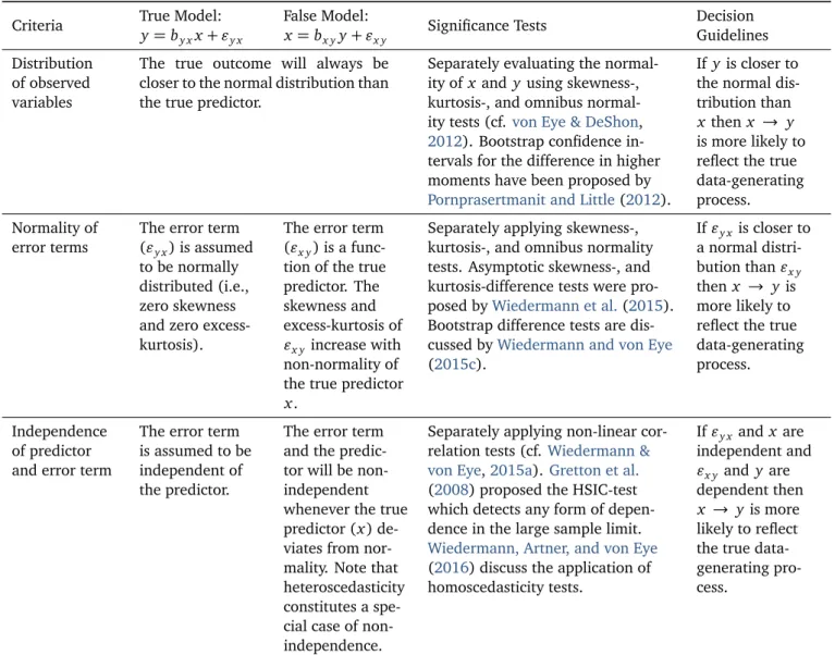
properties, which constitute the main components of DDA, concern 1) distributional characteristics of observed vari-ables (x and y), 2) distributional characteristics of the error terms obtained from competing regression models (x→ y versus y → x), and 3) independence properties of error terms and predictors of competing models. Table 1 summa-rizes these DDA components together with corresponding significance tests and decision guidelines. For simplicity, we restrict the presentation of DDA components to the bivari-ate case and refer to multiple variable extensions whenever possible.

Distributional Properties of Observed

Vari-ables

Asymmetric properties of observed variable distributions directly emerge from the additive nature of the linear re-gression model, i.e., an outcome variable is defined as the sum of two elements, a (non-normally distributed) ex-planatory variable and a (normally distributed) error term. Let

y= b_{y x}x+ "_{y x} (1)

be the true model describing the underlying data-generating process (for simplicity, but without loss of gen-erality, we assume that the intercept is fixed at zero). Here, xis assumed to be the cause of y with by x being the OLS

regression slope and "y x describing the error component

which is assumed to be normally distributed, serially inde-pendent, and independent of the predictor x. Further, let

x= bx yy+ "x y (2)

constitute the mis-specified model, i.e., the model that er-roneously treats y as the cause of variation in x.

Dodge and Rousson(2000,2001) as well asDodge and Yadegari(2010) showed that the Pearson correlationρx y= cov(x, y)/(σxσy) – with cov(x, y) being the covariance

andσxandσydenoting the standard deviations of x and y

– has asymmetric properties when considering higher mo-ments of x and y. Specifically, these authors show that the cube of the Pearson correlation can be expressed as the ratio of third moments of outcome and predictor (i.e., the skewness of outcome, γy, and the skewness of predictor, γx), ρ3 x y= γy γx . (3)

Similarly, the fourth power of the Pearson correlation can be written as the ratio of the fourth moments of outcome and predictor (i.e., the excess kurtosis of y, _κy, and the

excess kurtosis of x,_κx), ρ4 x y= κy κx . (4)

Because the Pearson correlation is bounded on the inter-val−1 and 1, it follows that the (absolute) skewness and

excess kurtosis1_{of the response variable y will always be}

smaller than the (absolute) skewness and excess kurtosis of the explanatory variable x. In other words, given that model (1) is capable of describing the data-generating pro-cess, the outcome variable y will be closer to the normal distribution than a non-normal predictor x. This funda-mental distributional property opens the door to evaluate the directional plausibility of a regression model through evaluating skewness and excess kurtosis of a tentative out-come and a tentative predictor. Note that this first DDA component is currently restricted to simple (bivariate) lin-ear regression settings which may hamper application in practice. The following two components, however, can be used to overcome this limitation.

Distributional Properties of Error Terms

Again, let model (1) be the true model and let model (2) be the directionally mis-specified model. The second DDA component focuses on the distributional shape of the er-ror terms associated with the two competing models, _"y x

and"x y. Wiedermann, Hagmann, Kossmeier, and von Eye

(2013),Wiedermann et al.(2015) as well asWiedermann (2015) showed that the skewness and the excess kurtosis of the error term obtained from the mis-specified model ("x y)

can be written as γ"x y = (1 − ρ 2 x y) 3/2_γ x (5) and κ"x y = (1 − ρ 2 x y) 2_κ x (6)

In other words, both, the third and the fourth moments of the false error term, can be expressed as functions of the third and fourth moments of the true predictor. From Equa-tions (5) and (6) one can conclude that the skewness and excess kurtosis of"x ysystematically increase with the

skew-ness and excess kurtosis of x. This relation has the natural interpretation that the amount of non-normality of x is re-flected in the “false” error term whenever the true predictor is erroneously used as the outcome variable. Because the true error term associated with the true model,"y x, is

as-sumed to follow a normal distribution (γ_{"y x} = κ_{"x y} = 0), systematic differences in higher moments of _"y x and"x y

may, again, inform researchers about the plausibility of the model in terms of directionality of an effect. Note that this DDA component can straightforwardly be extended to multiple-variable settings (seeWiedermann & von Eye, 2015b,2015c), i.e., to multiple linear regression models to draw conclusions about the directionality of effects in vari-able pairs (x, y) while adjusting for potential covariates (zj, j= 1, . . . , k).

1_{Note thatγ, κ, and ρ refer to the skewness, excess kurtosis, and the} Pearson correlation coefficient on the population level. Thus, while Equa-tions (3) and (4) will exactly hold in the population, one cannot expect the relations to hold exactly based on sample estimates. However, given that y= by xx+ "y xconstitutes the true underlying mechanism,γy/γx andκy/κxapproximate the third and the fourth power of the correlation coefficient with increasing sample size.

Table 1. Summary of DDA components.

Criteria True Model: False Model: Significance Tests Decision

y= b_{y x}x+ "_{y x} x= b_{x y}y+ "_{x y} Guidelines

Distribution of observed variables

The true outcome will always be closer to the normal distribution than the true predictor.

Separately evaluating the normal-ity of x and y using skewness-, kurtosis-, and omnibus normal-ity tests (cf. von Eye & DeShon, 2012). Bootstrap confidence in-tervals for the difference in higher moments have been proposed by Pornprasertmanit and Little(2012).

If y is closer to the normal dis-tribution than x then x → y is more likely to reflect the true data-generating process. Normality of

error terms

The error term ("y x) is assumed

to be normally distributed (i.e., zero skewness and zero excess-kurtosis).

The error term ("x y) is a

func-tion of the true predictor. The skewness and excess-kurtosis of "x yincrease with

non-normality of the true predictor x.

Separately applying skewness-, kurtosis-, and omnibus normality tests. Asymptotic skewness-, and kurtosis-difference tests were pro-posed byWiedermann et al.(2015). Bootstrap difference tests are dis-cussed byWiedermann and von Eye (2015c). If"y x is closer to a normal distri-bution than"x y then x → y is more likely to reflect the true data-generating process.

Independence of predictor and error term

The error term is assumed to be independent of the predictor.

The error term and the predic-tor will be non-independent whenever the true predictor (x) de-viates from nor-mality. Note that heteroscedasticity constitutes a spe-cial case of non-independence.

Separately applying non-linear cor-relation tests (cf.Wiedermann & von Eye,2015a). Gretton et al. (2008) proposed the HSIC-test which detects any form of depen-dence in the large sample limit. Wiedermann, Artner, and von Eye (2016) discuss the application of homoscedasticity tests. If_"y x and x are independent and "x yand y are dependent then x → y is more likely to reflect the true data-generating pro-cess.

Independence of Predictors and Error Term

The third DDA component focuses on the independence as-sumption of predictors and the corresponding error term. In essence, the independence assumption implies that the magnitude of error made in predicting scores of the out-come variable does not depend on the values of the pre-dictors. One essential feature of OLS estimation is that the estimated regression residuals will be uncorrelated with the predictors used in the model. It is important to note that uncorrelatedness will hold regardless of correctness of hy-pothesized path directions, i.e., both, the Pearson corre-lation of x and_"y x and the Pearson correlation of y and "x y will be zero by definition. However, uncorrelatedness

and (stochastic) independence are, in fact, two different concepts. Uncorrelatedness implies independence when all considered variables are normally distributed. However, in the non-normal case, uncorrelatedness does not necessar-ily imply independence. It can be shown that the inde-pendence assumption will be violated whenever the true predictor is erroneously used as the outcome of a regres-sion model. Because independence is assumed in the true model, decisions concerning the direction of effect are

pos-sible through separately evaluating the independence prop-erties of competing regression models (cf. Wiedermann & von Eye, 2015a). In the present article, we focus on ex-tending this asymmetric property of regression models to methods suited to answer research questions in the person-oriented context. Technical details together with a dis-cussion of how to statistically evaluate stochastic indepen-dence will be given below.

Competing Directional Theories in

Person-Oriented Research

In the following discussion, we take an intensive longitudi-nal data perspective, i.e., sufficiently frequently repeated measurements which allow conclusions about the sepa-rate developmental processes of single subjects, dyads, or pre-defined groups (Walls & Schafer,2006;Bolger & Lau-renceau, 2013). Intensive longitudinal designs are typi-cally applied to characterize change processes of subjects in their natural settings. AsBolger and Laurenceau(2013) note, “By characterize we mean not only functional form

of change but also its causes and consequences“ (p. 1). In other words, the intensive longitudinal data perspective is ideally-suited to empirically evaluate causal theories about complex (multi-variable) developmental processes. How-ever, many processes do not lend themselves to experimen-tation as the gold-standard for establishing causation (e.g., for ethical reasons). Further, even if randomization is feasi-ble, one still has to deal with the drawback that laboratory effects may not necessarily translate to real world settings. This situation clearly calls for methods that allow statisti-cal statements concerning the directionality of effects, i.e., a falsification-procedure for directional developmental the-ories.

Person- and variable-oriented approaches may share that often competing directional theories about phenomena of interest exist. While directional theories in the variable-oriented setting commonly concern mechanisms assumed to hold on a population level, person-oriented directional theories address variable relations and their complex de-velopment within the same subject. For example, various studies analyzed the relation (and causal ordering) of al-cohol consumption and intimate partner violence (IPV). From a variable-oriented perspective, it has been shown that IPV is indeed linked to alcohol consumption (see, e.g., Luthra & Gidycz,2006;Williams & Smith,1994). A person-oriented perspective is, for example, taken byKaterndahl, Burge, Ferrer, Becho, and Wood (2010). These authors used data of 16 women who were victims of domestic vi-olence. Study participants provided daily ratings on type and severity of violence together with estimates of the hus-band’s daily alcohol intake for 60 consecutive days. When analyzing the causal ordering of the two variables (alcohol intake and IPV) the following four possible (conceptual) models may be entertained: 1) alcohol intake causes sub-sequent IPV, 2) IPV causes subsub-sequent alcohol intake, 3) alcohol intake and IPV are related in feedback loops, and 4) IPV and AC are both caused by another, third factor (e.g., dysfunctional social interaction and relationship skills; cf. Downs, Smyth, & Miller,1996). Acknowledging that de-velopmental processes may be specific to the individual (as reflected in the first tenet of the person-oriented approach; Bergman & Magnusson,1997), we can expect that each of the four models will hold true in at least a subset of individ-uals. In other words, individual specificity is, of course, not restricted to idiosyncrasies in developmental trajectories of single characteristics. Individual specificity also implies variations in how several characteristics are causally related to each other. Further, causal relations within the same per-son may change over the life course. Returning to the ex-ample of IPV and alcohol consumption behavior, it may be true for some individuals that alcohol intake is responsi-ble for subsequent IPV. However, this may be followed by a later developmental stage were alcohol consumption of couples is used as a self-medicated coping strategy. Thus, both models, alcohol→ IPV and IPV → alcohol, may hold true depending on the developmental stage under consid-eration. In the following section, we propose extensions of DDA (originally proposed in the variable-oriented setting) to test competing directional theories of multiple

(longitu-dinally observed) variables.

Directional Dependence in Vector

Au-toregressive Models

An important difference between variable- and person-oriented analyses concerns the definition of the study sam-ple. While variable-oriented analyses typically focus on generalizations of model parameters obtained from a sam-ple of n participants to an a priori defined population, the person-oriented analysis considered here focuses on gener-alizations of an individual model. Measurement occasions of the same subject take the place of number of participants. Thus, generalizations concern the time dimension.

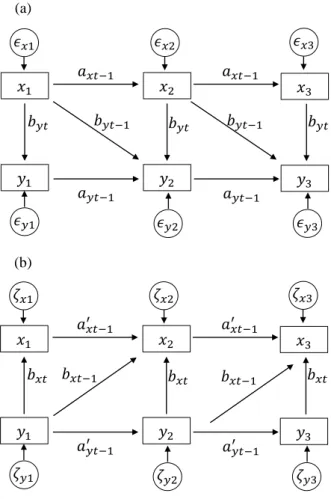
VAR modeling (e.g., Lütkepohl, 2007; Rovine & Lo, 2012) constitutes a straightforward approach to introduce DDA principles in the person-oriented domain. Let xt and y_t (t= 1, . . . , T) denote two stationary series of scores re-peatedly obtained from the same individual. Further, as-sume x scores contribute to the development of y, i.e., x is the (longitudinally observed) cause and y represents the (longitudinally observed) outcome. Figure 1a shows the conceptual path diagram of a (first-order) VAR model un-derlying x and y for three measurement occasions (note that the proposed approach is also valid for higher-order VARs, however, for notational simplicity, we restrict the pre-sentation to first-order VARs).

Here two different types of model parameters can be dis-tinguished, (first-order) autoregressive effects and cross-lagged effects. Autoregressive effects describe the expected change from one occasion t− 1 to the subsequent occa-sion t within the same variable (e.g., capturing the effect of past events of alcohol consumption on present and fu-ture drinking behavior). The parameter ax t−1 represents

the autoregressive effect of regressing xton xt−1and ay t−1

denotes the autoregressive effect of regressing yt on yt−1.

Cross-lagged parameters (by tand by t−1) describe the

con-tribution of the time series x in generating the time series y, i.e., the causal effects of x on y (e.g., the influence of alcohol consumption on IPV). Note that two different types of causal effect are considered in the present model, first-order lagged effects which represent the influence of xt−1

on ytand zero-order lagged effects (known as contempora-neous effects) describing the influence of xt on yt (reasons

for including contemporaneous effects will be discussed in detail below). The equations for this model can be written as

y_t= a_{y t−1}y_t−1+ b_{y t}x_t+ b_{y t−1}x_t−1+ "_{y t}

x_t= a_{x t−1}x_t−1+ "_{x t} (7)

where "y t and "x t denote the error terms of the model

which are assumed to be serially uncorrelated, indepen-dent of the corresponding predictors, and indepenindepen-dent of each other. The conceptualization of error components in time series models differs slightly from the definition of error terms in ordinary cross-sectional regression models. In a cross-sectional linear model such as the model given

𝑥𝑥

1

𝑥𝑥

2

𝑥𝑥

3

𝑦𝑦

1

𝑦𝑦

2

𝑦𝑦

3

𝑎𝑎

𝑥𝑥𝑥𝑥−1

𝑎𝑎

𝑥𝑥𝑥𝑥−1

𝑎𝑎

𝑦𝑦𝑥𝑥−1

𝑎𝑎

𝑦𝑦𝑥𝑥−1

𝑏𝑏

𝑦𝑦𝑥𝑥−1

𝑏𝑏

𝑦𝑦𝑥𝑥−1

𝜖𝜖

𝑥𝑥2

𝜖𝜖

𝑥𝑥3

𝜖𝜖

𝑥𝑥1

𝜖𝜖

𝑦𝑦1

𝜖𝜖

𝑦𝑦2

𝜖𝜖

𝑦𝑦3

𝑏𝑏

𝑦𝑦𝑥𝑥

𝑏𝑏

𝑦𝑦𝑥𝑥

𝑏𝑏

𝑦𝑦𝑥𝑥

𝑥𝑥

1

𝑥𝑥

2

𝑥𝑥

3

𝑦𝑦

1

𝑦𝑦

2

𝑦𝑦

3

𝑎𝑎

𝑥𝑥𝑥𝑥−1′

𝑎𝑎

𝑥𝑥𝑥𝑥−1′

𝑎𝑎

𝑦𝑦𝑥𝑥−1′

𝑎𝑎

𝑦𝑦𝑥𝑥−1′

𝑏𝑏

𝑥𝑥𝑥𝑥−1

𝑏𝑏

𝑥𝑥𝑥𝑥−1

𝜁𝜁

𝑥𝑥2

𝜁𝜁

𝑥𝑥3

𝜁𝜁

𝑥𝑥1

𝜁𝜁

𝑦𝑦1

𝜁𝜁

𝑦𝑦2

𝜁𝜁

𝑦𝑦3

𝑏𝑏

𝑥𝑥𝑥𝑥

𝑏𝑏

𝑥𝑥𝑥𝑥

𝑏𝑏

𝑥𝑥𝑥𝑥 (a) (b)

Figure 1. Path diagrams of competing VAR models.

in Equation (1), the error component usually captures measurement imprecision and variables outside the model. In contrast, in time series modeling the error component (sometimes referred to as “innovations”; cf. Lütkepohl, 2007) represents new information at a given measurement occasion t which influences the future development of a process. Thus, to evaluate hypotheses compatible with di-rection dependence, we assume that the error components in (7) are non-normally distributed.

Figure 1b shows the path diagram for the mis-specified model. Here, again, x is erroneously treated as the (repeat-edly observed) outcome and y serves as the (repeat(repeat-edly observed) cause of variation. This model takes the form

xt= a0x t−1xt−1+ bx tyt+ bx t−1yt−1+ ζx t

yt= a0y t−1yt−1+ ζy t, (8)

with a0_{x t−1}and a0_{y t−1} are the first-order autoregressive ef-fects, bx tand bx t−1describe the contemporaneous and the

first-order lagged effects of y on x, andζx tandζy tdenote

the error terms of the mis-specified model. In the follow-ing section, we show that DDA can be used to identify the correct VAR model (of course, assuming that it exists). We focus on the third DDA component which concerns the in-dependence of predictors and error terms.

Independence Properties of Predictors and

Er-rors in VAR Models

As discussed above, the decision of selecting between two directionally competing models can be based on separately evaluating whether the independence assumption is vio-lated. Assuming that the assumption of independent pre-dictor and error components is fulfilled in the “true” VAR model (e.g., x → y), we now show that the indepen-dence assumption will systematically be violated in a VAR model which erroneously considers a reversed causal flow ( y→ x).

The key element which allows to identify directional model-misspecifications is the so-called Darmois-Skitovich theorem (Darmois,1953;Skitovich,1953). These authors analyzed consequences of stochastic independence of lin-ear functions of variables. They showed that if two stochas-tically independent variables exist that are defined as the weighted sum of the same set of random variables (z), i.e.,

u= λ₁z₁+ λ₂z₂+ . . . + λ_kz_k

v= ξ₁z₁+ ξ₂z₂+ . . . + ξkzk (9)

with λ and ξ being non-zero values, then all variables z for which λξ 6= 0 follow a normal distribution (note that Mamai, 1963, extended this result to the case of infinite sums). From this, it straightforwardly follows that when at least one non-normal variable z exists for whichλξ 6= 0 is satisfied, u and v are stochastically dependent. Reconsider-ing the two competReconsider-ing VAR models given in Equations (7) and (8) reveals that the true outcome yt [which is

erro-neously treated as the predictor in Equation (8)] and the false error term ζx t are both linear combinations of the samevariables and, thus, fulfill the requirements to apply the Darmois-Skitovich theorem. This can be shown by, first, re-writing the “true“ model (7) as

yt = ay t−1yt−1+(by tax t−1+by t−1)xt−1+by t"x t+"y t (10)

(which is obtained through inserting the autoregressive component of xt into the equation describing the

develop-ment of yt) and, second, solving the mis-specified model

given in (8) for the error term _ζx t after inserting the true

into the mis-specified model which results in

ζx t= (1−bx tby t)"x t−θx t−1xt−1−θy t−1yt−1− bx t"y t (11)

withθx t−1= (ax t−1− ax t−1bx tby t− bx tby t−1− a0x t−1) and

θy t−1 = (ay t−1bx t+ bx t−1). From (10) and (11) we

con-clude that both, yt andζx t, are linear combinations of 1)

past y values, yt−1, 2) past x value, xt−1, 3) the “true“

error term "x t, i.e., innovations of xt, and 4) the “true“

error term "y t, i.e., innovations of yt. Thus, it follows

from the Darmois-Skitovich theorem that yt andζx t will

be stochastically dependent if 1) the error component"x t

is non-normally distributed and by t(1− bx tby t) 6= 0 and/or

2) the error component"y tis non-normal and bx t6= 0.

Fi-nally, assuming that the independence assumption holds for the true model, we arrive at the following simple guidelines to select between directionally competing models:

• If the independence assumption holds for xt and"y t

and, at the same time, the independence assumption is violated for yt and ζx t then the model x → y is

more likely to approximate the true data-generating process.

• If the independence assumption holds for yt andζx t

and, at the same time, the independence assumption is violated for xt and"y t then the model y → x is

more likely to approximate the true data-generating process.

• If the independence assumption is violated in both models then unmeasured confounders may be present and no distinct decision on the direction of effect can be made. If the independence assumption is fulfilled in both models then no decision can be made. Note that this scenario points at violated distributional re-quirements and/or power issues due to small sample size.

Testing Independence

The selection procedure described above relies on testing independence of predictors and error terms. In practice, residuals will be used to approximate the unknown error components. Because regression residuals and the predic-tor will be uncorrelated by definition, evaluating indepen-dence of the two components becomes more complex. We focus on two promising approaches: 1) Non-linear corre-lation approaches and 2) a kernel-based test for statistical independence.

Non-Linear Correlation Approaches. These statistical approaches emerge from the fact that (stochastic) inde-pendence is a much stronger assumption than uncorrelat-edness. While uncorrelatedness refers to the situation of zero-covariances of pairwise variables, independence im-plies that zero-covariances exist for any non-linear func-tions of the pairwise variables (cf. Hyvärinen, Karhunen, & Oja,2001). In practice, this implies that correlation tests can be applied on (non-linearly) transformed variables to evaluate stochastic non-independence. In other words, in-stead of testing the null hypothesis of zero correlation of y_t and ζx t (which will be zero by definition), one

eval-uates whether zero-correlations hold for, e.g., {y_t2, ζ2_{x t}}, {exp(yt), sin(ζx t)}, {tanh(yt), ζx t}, etc. Of course,

test-ing all possible non-linear transformations is not feasible in practice, which raises the important question which non-linear transformation should be applied to make statements about potential non-independence of predictor and residu-als. Wiedermann and von Eye (2015a, 2016) as well as Wiedermann et al.(2016) showed that squaring the vari-ables, i.e., {y2

t, ζx t} and {yt, ζ2x t}, is particularly useful

to detect non-independencies because covariances of{y2 t, ζx t} and {yt,ζ2x t} increase with the skewness of the “true”

predictor. Assuming that both estimated models (7) and (8) show adequate model fit (i.e., to be considered eligible as competing candidates, both models should fit the data well in terms of second order moments) and making use

of the proposed decision guidelines results in the following model selection procedure:

• If the null hypotheses H0 : cor(x2t,"y t) = 0 and H₀ : cor(xt,"2y t) = 0 are both retained and, at the

same time, at least one of the null hypotheses H0 :

cor(y_t2,ζx t) = 0 and H0: cor(yt,ζ2x t) = 0 is rejected

then the model x → y is more likely to approximate the true data-generating process.

• If the null hypotheses H0 : cor(yt2,ζx t) = 0 and H₀ : cor(yt,ζ2x t) = 0 are both retained and, at the

same time, at least one of the null hypotheses H₀ : cor(x2_t,"y t) = 0 and H0: cor(xt,"2y t) = 0 is rejected

then the model y → x is more likely to approximate the true data-generating process.

• If null hypotheses of zero (nonlinear) correlations are rejected in both models then unmeasured confounders are likely to be present. Hence, no decision can be made.

• If null hypotheses of zero (nonlinear) correlations are retained in both models, no distinct decision can be made (this again points at low power or violated data requirements).

This independence approach has the advantage of com-putational simplicity. In fact, given that the test statistics rely on the ordinary Pearson correlation test, this approach is readily available in virtually all statistical software pro-grams. However, applying this approach introduces ad-ditional Type II error risks (aside of Type II error due to small sample sizes), because retaining null hypotheses of zero correlation for selected non-linear functions does not guarantee that no other non-linear functions may exists for which non-independence hold. The following kernel-based test can be used to overcome these limitations.

Kernel-Based Independence Test. Gretton et al.(2008) introduced a kernel-based approach for testing indepen-dence, the so-called Hilbert-Schmidt Independence Cri-terion (HSIC). Instead of analyzing independence prop-erties of random variables, the HSIC deals with test-ing the independence of functions of random variables. Thus, the HSIC approach is provably universal in de-tecting any dependence between two random variables. Due to space restrictions, we do not present techni-cal details of the test statistic (for details see Gretton et al., 2008). This approach may have the disadvan-tage of high computational complexity. Further, the test is not readily available in standard statistical software programs (Matlab implementations of the test can be found at

http://www.gatsby.ucl.ac.uk/~gretton/

indepTestFiles/indep.htm). Again, making use of

the proposed decision guidelines, we arrive at the follow-ing model selection procedure (of course, again, both can-didate models should fit the data well in terms of second order moments):

• If the null hypothesis of the HSIC-test H0: xt ⊥ "y t

(i.e., xt and"y tare stochastically independent) is

re-tained and, at the same time, at the null hypothesis H₀ : yt ⊥ ζx t is rejected, then the model x → y is

more likely to approximate the true data-generating process.

• If the null hypothesis H0 : yt ⊥ ζx t is retained and,

at the same time, at the null hypothesis H0: xt ⊥ "y t

is rejected, then the model y → x is more likely to approximate the true data-generating process. • If both null hypotheses are rejected then unmeasured

confounders are likely to be present.

• If both null hypotheses are retained, no distinct deci-sion concerning the direction of effect can be made.

Empirical Example: Subjective Mood

and Alcohol Consumption Behavior

In the following section, we illustrate how to apply the proposed methodology in practice. We use data from a study on the development of alcoholism of adults who self-identified as alcoholics (Perrine, Mundt, Searles, & Lester, 1995). Using automated interviews, daily alcohol con-sumption (i.e., number of alcoholic beverages), together with daily subjective mood, stress, and health ratings were obtained over a study period of three years. Various pre-vious studies analyzed this dataset from a person-oriented perspective (von Eye & Bergman, 2003;von Eye & Mun, 2012; von Eye et al., 2015). For example, von Eye and Wiedermann (2016, this issue) use daily recorded alco-hol consumption to illustrate configural models to answer whether there exist interindividual differences in intraindi-vidual change. In the following application, we ask ques-tions concerning the direction of effect of subjective mood and alcohol consumption behavior from a person-oriented perspective, i.e., whether individual changes in mood are the cause of changes in alcohol consumption (i.e., mood → alcohol) or whether alcohol consumption patterns cause changes in perceived mood (i.e., alcohol → mood) for a single subject. Specifically, we analyze time series data of one participant (respondent 3032) based on observed weekly aggregates. Note that both competing VARs may have theoretical support: The well-established “tension re-duction hypothesis” (Conger,1956;Young, Oei, & Knight, 1990), where (negative) mood is assumed to prompt alco-hol use as a self-medication approach, poses that a model of the form mood→ alcohol explains the observed develop-ment over time. In contrast, the “hedonic motive hypothe-sis” (Gendolla,2000) states that alcohol may reinforce the mood which, in turn, supports a model of the form alcohol → mood.

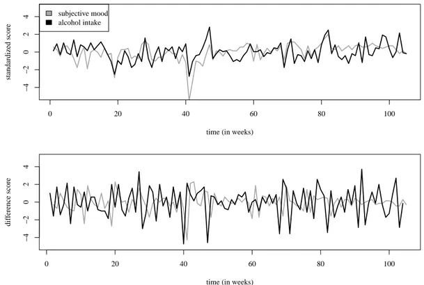
Figure 2 (upper panel) shows the standardized scores of observed (weekly averaged) mood ratings together with the (weekly averaged) number of alcoholic beverages for 105 consecutive weeks. To remediate potential issues of non-stationarity of both time series, first-order differences

between observations ( y0

t = yt− yt−1and x0t= xt− xt−1)

were computed. Thus, time series used in VAR-DDA reflect the observed change between each observation in the origi-nal series. Figure 2 (lower panel) shows the differenced se-ries for perceived mood and alcohol intake. The KPSS-test (Kwiatkowski, Phillips, Schmidt, & Shin, 1992) indicated stationarity of both differenced series (both p’s> .1).

Next, for both directionally competing models, mood → alcohol (Model I) and alcohol → mood (Model II), the Bayesian Information Criterion (BIC) was used to select proper lag length (cf. Lütkepohl,1985). For both possible directions (mood→ alcohol and alcohol → mood) a series of VAR model were estimated and lagged values up to the fifth order were considered for the corresponding predictor variables. For Model I, including first- and second-order lags for alcohol intake and first-order lags for mood ratings showed the lowest BIC. For Model II, the lowest BIC was observed when considering first-, second-, and third-order lags for subjective mood ratings and first-order lags for al-cohol consumption (the Durbin-Watson test confirmed the absence of autocorrelation of disturbances for both mod-els; both p’s> .7). Before we can interpret the parameter estimates of the models, it is important to ensure that both candidate models describes the data well in terms of second moments. Model I showed a multiple R2of 0.45[F(4, 97) = 19.86, p < .001], for Model II we obtained a multiple R2 of 0.38 [F(5, 95) = 11.75, p < .001]. Further, the model goodness of fit test suggested that both models are able to describe the data well[Model I: χ2(2) = 1.89, p = .389; Model II:χ2(3) = 3.60, p = .308]. Figure 3 shows the path diagrams together with the estimated coefficients of both models. In general, interpretations of parameter estimates for both models are complementary in nature. For Model I, we observe that past increases in alcohol consumption lead to a decrease in present alcohol intake (the effects of past alcohol intake decrease with lag length) while present alco-hol consumption increases with past and present mood (the impact of mood also decreases with lag length). For Model II, we obtain a complementary picture, i.e., past increases in mood lead to decreases in present mood while present mood increases with past and present alcohol consumption (again, all effects decrease with lag length).

In the next step, we ask questions concerning the direc-tion of effect. Note that the presented direcdirec-tion depen-dence approach relies on the assumption of non-normally distributed error terms. Thus, we, first, computed the re-gression residuals of both models and checked whether we find empirical support for this distributional assumption in at least one of the two models. Residuals of Model I showed a skewness of 0.24 and an excess kurtosis of –0.54. The Kolmogorov-Smirnov test rejected the null hypothesis of normally distributed residuals (D = 0.13, p = .047). For residuals of Model II, we obtained a skewness of –1.09 and an excess kurtosis of 2.07. Here, the Kolmogorov-Smirnov test retained the null hypothesis of normality according to the 5% nominal significance level (D = 0.12, p = .121). However, overall, we can conclude that the residuals are sufficiently non-normal to proceed with testing direction dependency.

0 20 40 60 80 100 −4 −2 0 2 4

time (in weeks)

standardized score

subjective mood alcohol intake

time (in weeks)

dif ference score 0 20 40 60 80 100 −4 −2 0 2 4

Figure 2. Observed time series for respondent 3032 (upper panel: Observed weekly averaged mood ratings and weekly averaged number

of alcoholic beverages; lower panel: First-order differenced time series).

Three non-linear correlation tests using the squaring function and the HSIC-test were used to evaluate the independence assumption for both models. For Model I, all non-linear correlation tests were non-significant: cor(moodt,"2al c) = −0.12, p = .214; cor(mood

2

t,"al c) =

−0.13, p = .183; cor(mood2t," 2

al c) = −0.11, p = .294.

Fur-ther, the HSIC-test confirmed independence of predictor and error term (HSIC_{= 0.25, p = .650). In contrast, all} non-linear correlation tests rejected the independence as-sumption for Model II: cor(alct,"mood2 ) = −0.22, p = .026; cor(alc2_t,_"mood) = −0.23, p = .022; cor(alc2t,"

2 mood) =

0.40, p< .001. The HSIC-test failed to reject the null hy-pothesis (HSIC = 0.44, p = 0.188). Applying the deci-sion guidelines proposed above, we conclude that a model of the form (Model I) is more likely to describe the data-generating process based on non-linear correlation tests. The HSIC-test does not allow a distinct decision because null hypotheses for both models were retained. One rea-son for this may be the rather small sample size (i.e., short time series) which reduces the power of the test. How-ever, we observe a larger HSIC value for Model II indicat-ing a larger magnitude of non-independence compared to Model I (0.44 versus 0.25) which again, points toward the model mood→ alcohol. Thus, overall, DDA suggests that (for respondent 3023) experienced mood is more likely to cause alcohol intake than vice versa which is in line with the “tension-reduction hypothesis”.

Discussion

The present study introduced basic principles of DDA to person-oriented researchers and presented extensions of DDA to VAR models which can be used to study change in single subjects. The presented approach allows one to study directionality of functional relations observed over time and thus matches the notion of individual causality (cf. Bergman,2009). In the following paragraphs, we start with briefly summarizing the results of extensive Monte-Carlo simulation experiments (assessing the Type I error and power performance of the proposed approach) to pro-vide guidelines for practical applications. Further, it is im-portant to reiterate that the VAR model considered here differs in two important aspects from “traditional” models: First, to apply direction dependence principles, we assume that the error terms of the model deviate from the normal distribution. Second, we consider contemporaneous effects (i.e., effects which occur at the same measurement occasion t) in addition to lagged effects of the two series. We discuss the plausibility of these requirements from both, practical and methodological perspectives. Finally, we close the arti-cle with outlining further applications of DDA in the person-oriented domain.

Type I Error and Power Considerations

We have conducted extensive Monte-Carlo simulation ex-periments to assess the Type I error and power performance of the proposed model selection procedure. Here, we sum-marize simulation results focusing on the length of the time

𝑀𝑀1 𝑀𝑀2 𝑀𝑀3 𝑀𝑀4 𝐴𝐴𝐴𝐴1 𝐴𝐴𝐴𝐴2 𝐴𝐴𝐴𝐴3 𝐴𝐴𝐴𝐴4 0.379 0.379 0.379 0.705 0.705 0.705 0.705 –0.213 –0.213 –0.637 –0.637 –0.637 –0.303 –0.303 –0.303 𝑀𝑀1 𝑀𝑀2 𝑀𝑀3 𝑀𝑀4 𝐴𝐴𝐴𝐴1 𝐴𝐴𝐴𝐴2 𝐴𝐴𝐴𝐴3 𝐴𝐴𝐴𝐴4 0.175 0.301 0.301 0.301 0.301 –0.297 –0.297 –0.469 –0.469 –0.469 –0.472 –0.472 –0.472 –0.175 0.175 0.175 Model I Model II

Figure 3. Results of competing VAR models for mood and

alco-hol consumption (all coefficients in both models are statistically significant using a nominal significance level of 5%; AC= alcohol consumption, M= perceived mood).

series, the degree of asymmetry of error term distributions, and effect sizes of autoregressive, lagged, and contempora-neous effects.

As expected, nonlinear correlation approaches of the form cor(y2

t,ζx t) and cor(yt,ζ2x t) were able to protect the

nominal significance level of 5% when error terms were randomly sampled from a normal distribution. Empirical Type I error rates of the HSIC were systematically lower than 5%. In general, empirical power to select the cor-rect VAR model increases with the skewness of the error terms, the length of the time series, and the magnitude of the contemporaneous effect. In contrast, the power slightly decreases with the magnitude of autoregressive and cross-lagged effects. With respect to Cohen’s (1988) defi-nition of small, medium, and large effects, the following rough guidelines can be used in order to achieve a power of 80%: First, for large contemporaneous effects together with skewness values of the error terms larger than 1.5, T ≥ 100 observations are necessary for medium autore-gressive effects (T≥ 50 may be sufficient for small autore-gressive effects). Second, for medium-sized contemporane-ous effects, T≥ 200 observations are necessary to achieve a power of 80%. Third, the nonlinear correlation test of the form cor(yt,ζ2x t) is more powerful than the HSIC-test.

Cor-relation approaches of the form cor(y_t2,ζx t) showed the

lowest power.

Non-Normal Errors

Various studies repeatedly demonstrated that the normal-ity assumption is very likely to be violated in empiri-cally observed data. For example, Micceri (1989) ana-lyzed over 440 empirical datasets regarding their distri-butional properties and found that only 4.3% were rea-sonably normal while the Kolmogorov-Smirnov test indi-cated non-normality for all 440 distributions at a 1% signif-icance level. Quite similar results were obtained byBlanca, Arnau, López-Montiel, Bono, and Bendayan (2013) who studied 693 empirically observed distributions (measures of cognitive ability and other psychological variables) and found that only 5.5% were approximately normally dis-tributed. One theoretical explanation why variables (and error terms) are likely to deviate from the normal distribu-tion is, for example, given byBeale and Mallows(1959). The error term of a model usually captures measurement error and unconsidered background variables. Now, as-sume that the error is a mixture of several unobserved in-dependent and normally distributed variables (zj). In this

case, the resulting error term will show elevated excess kur-tosis values whenever the variances of the unconsidered variables, zj, differ from each other. Because unequal

vari-ances are likely to occur in practice, the error terms are also likely to deviate from normality (note that the same argu-ment applies to the predictor variable of a model). From these results, we may conclude that distributional require-ments of DDA are very likely to hold in practical applica-tions.

However, the assumption of non-normal error terms de-viates from the classic VAR set-up. In the classic VAR model, testing for non-normality of error terms is commonly rec-ommended as a model-checking procedure (Lütkepohl, 2007) where non-normality of residuals may indicate that additional variables or lag structures improve the model. However, it is important to note that non-normality may still exist after including additional variables and/or addi-tional higher order lags. The VAR-DDA approach presented here differs from the classical set-up in the sense that non-normality may not only be used to indicate potential model-misspecification of the predictor side of the model equation. Considering non-normality as a valuable source of infor-mation enables researchers to identify directional model-misspecifications.

Note that this is not the first study which makes use of higher than second moment information of time series data. For a discussion of non-normality in the time series domain see, for example, Granger and Newbold (1976), Swift and Janacek(1991) andSim(1994). Further,Peters, Janzing, Gretton, and Schölkopf (2009) evaluate the re-versibility of autoregressive moving average (ARMA) mod-els through testing the independence of the error terms and preceding values of the time series. More recently, Hernández-Lobato, Morales-Mombiela, and Suárez(2011) showed that time-reversed residuals of linear ARMA mod-els will always be closer to the normal distribution than non-normal true errors of the chronologically ordered time series (i.e., a so-called Gaussianization effect). Hyvärinen, Zhang, Shimizu, and Hoyer (2010) proposed an

exten-sion of the so-called linear non-Gaussian acyclic model (LiNGAM; cf. Shimizu, Hoyer, Hyvärinen, & Kerminen, 2006) – in essence, a causal discovery algorithm used to recover the underlying structure of directed acyclic graphs (DAG) – to VAR models. Conceptual differences of DDA and causal discovery algorithms are discussed byWiedermann and von Eye(2015a).

Considering Contemporaneous Effects

Often, researchers are reluctant to consider contemporane-ous effects in VAR models for reasons rooted in properties of the model resulting from second order moments of vari-ables (variances and covariances). Consider, for example, so-called Granger-causality testing (Granger, 1969) which was originally introduced in the econometric sciences but also received considerable attention in various life sciences domains such as studying effective connectivity of neurons using fMRI data (see, e.g., Stephan & Roebroeck, 2012) or studying gene regulatory networks (Lozano, Abe, Liu, & Rosset,2009). In essence, Granger causality testing con-stitutes a predictor error approach. Here, a time series x is said to “Granger-cause“ another time series y, when additionally including past information of x in the tion of y leads to a better model fit (i.e., a smaller predic-tor error) than predicting y from its own past alone. In-terestingly, although temporal information may be seen as the key ingredient for causal claims (implicitly following Hume’s proposition that the cause must precede the effect, Granger, 1969) also considered contemporaneous effects of x and y. However, contemporaneous effects are rarely considered in practice because the direction of contem-poraneous effects cannot be derived from standard VARs (see,Hsiao,1982; Lütkepohl,2007). From this perspec-tive, including higher order information to identifying the direction of effects, may also resolve an important issue in Granger-causality testing (see alsoHyvärinen et al.,2010; von Eye & Wiedermann,2015).

As noted above, the fact that contemporaneous effects tend to be ignored in time series modeling, may be deeply rooted in sequential theories of causation (Hume, 1777; Mill,1851) where temporality is an essential requirement to establish causation. Of course, from a purely statistical perspective, sequential ordering of variables alone is known to be insufficient to establish causation, i.e., longitudinal in-formation does not rule out spurious correlations over time (Yule,1921,1926;Link & Shrout,1992). Further, consid-ering that even many physical laws are, in fact, formulated in a time-reversible form2 _{lends support to theories of}

si-multaneous causationwhich focus on physical mechanisms underlying the process of interest and pose that temporally extended outcomes occur simultaneously with temporally extended causes (Huemer & Kovitz,2003). Another argu-ment which may further substantiate the inclusion of con-2_{For example, the well-known relation between force ( f ), mass (m),} and acceleration (a), f = ma, may entice the view that force is caused by mass and acceleration. However, this fundamental relation does not necessarily imply a specific direction of time, i.e., using a= f /m one may easily conclude that acceleration is caused by force and mass (cf.Huemer & Kovitz,2003).

temporaneous effects concerns the measurement of time series itself. While change over time is typically concep-tualized as being incessant and continuous (Lerner,1998), time series data (obtained to measure change) are collected using fixed measurement intervals (i.e., the amount of time that elapses between measurement occasions often is con-sidered constant; for a methodological discussion of tempo-ral designs seeTimmons & Preacher,2015). Reconsider the empirical example on subjective mood and alcohol intake: The respondent’s mood, which may impact the alcohol con-sumption behavior, is (consciously or subconsciously) ex-perienced in a continuous manner. Even if respondents are requested to provide information about their prior day‘s ex-periences and behaviors, not considering contemporaneous information implies that potential change that occurs in be-tween two consecutive measurement occasions is consid-ered as being unimportant for the process of modeling the relation of the two phenomena of interest. From this per-spective, omitting potential contemporaneous effects may be seen as an unnecessary truncation of available informa-tion. Further, for the social sciences, it is important to note that concepts of contemporaneous effects may differ from standard conceptualizations of simultaneous causation typ-ically used in philosophical accounts. While philosophical discussions consider contemporaneous causal effects as ing truly immediate (i.e., there is no time difference be-tween two causally related events), contemporaneous ef-fects in the social sciences may be better understood as the result of measurement within a short period of time which is commonly assumed to be negligible for the quantifica-tion of change. However, even short periods of time may provide enough room for a temporal ordering of variables which, again, lends support to incorporating contempora-neous effects in the analysis of functional relations.

Potential Extensions of DDA in the

Person-Oriented Domain

Because principles of DDA concern the linear model in its general definition as an additive error model various exten-sions in both, the variable- and person-oriented domain, are possible. In the variable-oriented setting, for exam-ple, extensions to mediation models have been discussed by Wiedermann and von Eye (2015b) and Wiedermann and von Eye (2016). Acknowledging that many person-oriented methods rely on the linear model implies that DDA may also be applied in other person-oriented settings which definitely warrants future research.

For example,von Eye et al.(2015) as well asAsendorpf (2015) discuss hierarchical linear modeling (HLM) as an important methodological tool compatible with the person-oriented perspective. In essence, HLM considers a hi-erarchically nested data structure (e.g., repeated mea-sures nested within respondents) and allows one to ex-amine level-specific variation (i.e., HLM explicitly mod-els inter- and intraindividual differences). Because the level-specific error terms are assumed to be independent and normally distributed random variates, systematic viola-tions of these assumpviola-tions may point at directional

model-misspecifications.

Further, dynamic factor models (Molenaar,1985;Wood, 2012) have been identified as ideally-suited to study the tenets of person-oriented research (cf., Molenaar, 2010). The dynamic factor model can be written as

yt= Ληt+ "t

ηt= B1ηt−1+ B2ηt−2+ . . . + Bsηt−s+ ζt, (12)

with yt being a p-variate manifest time series (t =

1, . . . , T ),_ηtis a q-variate time series of latent factor scores, Λ denotes p × q matrix of factor loadings, and "t is a

p-variate error time series capturing specific and measure-ment error. Further, ηt is modeled as a function of prior

latent states weighted by Bk(k= 1, . . . , s) while ζt denotes

present-time “innovations” (i.e., the error component rep-resenting new information at a given time point). In addi-tion to lagged and cross-lagged effects of latent factors, con-temporaneous latent variable effect may be incorporated as well. Note that present “innovations” are assumed to be independent of latent states on the predictor side of the model which may open the door to apply principles of DDA to evaluate directional hypotheses of latent contemporane-ous effects in dynamic factor models.

References

Asendorpf, J. B. (2015). Person-oriented approaches within a multi-level perspective. Journal for Person-Oriented

Re-search, 1, 48–55.

Beale, E. M. L., & Mallows, C. L. (1959). Scale mixing of symmet-ric distributions with zero means. Annals of Mathematical

Statistics, 30, 1145–1151.

Bergman, L. R. (2009). Mediation and causality at the individual level. Integrative Psychological and Behavioral Science, 43, 248–252.

Bergman, L. R., & Lundh, L. G. (2015). The person-oriented approach: Roots and roads to the future. Journal of

Person-Oriented Research, 1, 1–6.

Bergman, L. R., & Magnusson, D. (1997). A person-oriented ap-proach in research on developmental psychopathology.

De-velopment and Psychopathology, 9, 291–319.

Bergman, L. R., Magnusson, D., & El Khouri, B. M. (2003).

Studying individual development in an interindividual con-text: A person-oriented approach. Mahwah, NJ: Lawrence Erlbaum.

Blanca, M. J., Arnau, J., López-Montiel, D., Bono, R., & Bendayan, R. (2013). Skewness and kurtosis in real data samples.

Methodology, 9, 78–84.

Bolger, N., & Laurenceau, J. P. (2013). Intensive longitudinal

meth-ods: An introduction to diary and experience sampling re-search. New York: Guilford Press.

Cohen, J. (1988). Statistical power analysis for the behavioral

sciences(2nd ed.). Hillsdale, NJ: Erlbaum.

Conger, J. J. (1956). Reinforcement theory and the dynamics of alcoholism. Quarterly Journal of Studies on Alcohol, 17, 296–305.

Darmois, G. (1953). Analyse générale des liaisons stochastique [General analysis of stochastic links]. Review of the

Interna-tional Statistical Institute, 21, 2–8.

Dodge, Y., & Rousson, V. (2000). Direction dependence in a regres-sion line. Communications in Statistics: Theory and Methods,

29, 1957–1972.

Dodge, Y., & Rousson, V. (2001). On asymmetric properties of the correlation coefficient in the regression setting. The

Ameri-can Statistician, 55, 51–54.

Dodge, Y., & Yadegari, I. (2010). On direction of dependence.

Metrika, 72, 139–150.

Downs, W. R., Smyth, N. J., & Miller, B. A. (1996). The rela-tionship between childhood violence and alcohol problems among men who batter: An empirical review and synthesis.

Aggression and Violent Behavior, 1, 327–344.

Galton, F. (1886). Regression towards mediocrity in hereditary stature. Journal of the Anthropological Institute of Great

Britain and Ireland, 15, 246–263.

Geldhof, G. J., Bowers, E. P., Johnson, S. K., Hershberg, R., Hilliard, L., & Lerner, R. M. (2014). Relational devel-opmental systems theories of positive youth development: methodological issues and implications. In P. C. M. Mole-naar, R. M. Lerner, & K. M. Newell (Eds.), Handbook of

de-velopmental systems theory and methodology (pp. 66–94). New York: Guilford Press.

Gendolla, G. H. E. (2000). On the impact of mood on behav-ior: An integrative theory and a review. Review of General

Psychology, 4, 378–408.

Granger, C. W. J. (1969). Investigating causal relations by econo-metric models and cross-spectral methods. Econoecono-metrica,

37, 424–438.

Granger, C. W. J., & Newbold, P. (1976). Forecasting transformed series. Journal of the Royal Statistical Society B, 38, 189– 203.

Gretton, A., Fukumizu, K., Teo, C. H., Song, L., Schölkopf, B., & Smola, A. J. (2008). A kernel statistical test of indepen-dence. Advances in Neural Information Processing Systems,

20, 585–592.

Hanley, J. A. (2004). “Transmuting” women into men: Galton’s family data on human stature. American Statistician, 58, 237–243.

Hernández-Lobato, J. M., Morales-Mombiela, P., & Suárez, A. (2011). Gaussianity measures for detecting the direction of causal time series. In Proceedings of the international

joint conference on artificial intelligence(Vol. 22, pp. 1318– 1323).

Hsiao, C. (1982). Autoregressive modeling and causal ordering of economic variables. Journal of Economic Dynamics and

Control, 4, 243–259.

Huemer, M., & Kovitz, B. (2003). Causation as simultaneous and continuous. Philosophical Quarterly, 53, 556–565. Hume, D. (1777). Enquiries concerning human understanding

and concerning the principles of morals. Oxford: Clarendon Press.

Hyvärinen, A., Karhunen, J., & Oja, E. (2001). Independent

com-ponent analysis. New York: Wiley & Sons.

Hyvärinen, A., Zhang, K., Shimizu, S., & Hoyer, P. O. (2010). Es-timation of a structural vector autoregression model using non-gaussianity. Journal of Machine Learning Research, 11, 1709–1731.

Katerndahl, D. A., Burge, S. K., Ferrer, R. L., Becho, J., & Wood, R. (2010). Complex dynamics in intimate partner violence: A time series study of 16 women. Primary Care Companion to

the Journal of Clinical Psychiatry, 12(4).

Kwiatkowski, D., Phillips, P. C. B., Schmidt, P., & Shin, Y. (1992). Testing the null hypothesis of stationarity against the alter-native of a unit root. Journal of Econometrics, 54, 159–178. Lerner, R. M. (1998). Theories of human development:

Contem-porary perspectives. In W. Damon & R. M. Lerner (Eds.),

Handbook of child psychology: Theoretical models of human development(5th ed., pp. 1–24). New York: Wiley.