02:23 Pourbaix Diagrams for Copper in 5 m Chloride Solution

(1)

SKI Report 02:23

Research

Pourbaix Diagrams for Copper

in 5 m Chloride Solution

Björn Beverskog

Sven-Olof Pettersson

December 2002

(2)

SKI perspective

Background

The integrity of the canister is an important factor for the long-term safety of the repository for spent nuclear fuel. The outer copper shell gives corrosion protection, while the cast iron insert gives mechanical integrity. The resistance against corrosion must be studied in the different environments that can be possible in a final repository, e.g. highly saline solutions.

The corrosion behaviour of copper can be studied by thermodynamic calculations of the stability areas of copper and copper compounds. The results can also be compared to experiments.

Purpose of the project

The purpose of this study was to calculate Pourbaix diagrams (potential – pH diagrams) for copper in 5 molal chlorine solution as an extension of earlier work on lower chlorine concentrations (0.2 and 1.5 molal).

Results

The main conclusion of this study is that chloride reduces both the immunity and

passivity areas of copper, and that copper will corrode in 5 m chlorine solution at 100°C at repository potentials and pH. Copper can corrode at lower temperatures depending on the copper concentration.

Further, if there are no macro cracks in the bentonite clay, the copper and the bentonite could be viewed as a closed system. The limited diffusion of oxygen inwards and corrosion products outwards, will then cause the corrosion potential to fall into the immunity area of copper. The corrosion of the copper will then automatically stop.

Effects on SKI work

The results of the calculations will be used in experimental studies of the corrosion behaviour of copper in highly saline solutions. These studies will be one basis for coming SKI reviews of SKB’s programme for disposal of spent nuclear fuel, such as review of SKB’s RD&D Programme 2004 and review of SKB’s application to build an

(3)

SKI Report 02:23

Research

Pourbaix Diagrams for Copper

in 5 m Chloride Solution

Björn Beverskog¹

Sven-Olof Pettersson²

¹OECD Halden Reactor Project

Institutt før Energiteknikk

Box 173

N-1751 Halden

Norway

²ChemIT

S-611 45 Nyköping

Sweden

December 2002

This report concerns a study which has been conducted for the Swedish Nuclear Power Inspectorate (SKI). The conclusions

(4)

List of contents

Abstract 3 Sammanfattning 4 1 Introduction 5 2 Choice of species 7 2.1 Chlorine - water 7 2.2 Copper - water 8

2.3 Copper - chlorine - water 9

3 Thermochemical data 11

3.1 Solids 11

3.2 Aqueous species 12

4 Calculations 15

5 Result and discussion 17

5.1 General behavior 17

5.2 Corrosion of copper at repository potentials, pH and temperatures 19 5.3 Corrosion of copper canisters in a deep repository 20

6 Conclusions 23

Acknowledgments 25

References 27

(5)

1 Introduction

The spent nuclear fuel in Sweden and Finland will be encapsulated into metal canisters, according to the KBS-3 concept developed by SKB†_{. The fuel will be encapsulated in a}

canister of iron, which is chosen due to its mechanical properties. The iron canister will be encapsulated in a copper canister (5 cm thick), which is chosen due its excellent corrosion properties. Copper is choosen as it is assumed to be in its immune state in the anoxic environment at 500 m down in the granite bedrock. The ground water circulating in the fractured of the bedrock surrounding the repository can be low in chloride content to highly saline.

The canisters will embedded in a buffer of compacted bentonite clay. The temperature at the canister surface will have an initial maximum of ∼ 80°C , due to the heat

produced by the spent nuclear fuel. Whether the radiation level is high enough to produce radiolysis of water at the copper surface is not yet fully clear.

To predict the corrosion behavior of a metal from thermodynamic calculations it is essential to consider all the species that the metal can form with the components of the environment. As copper has a strong affinity for chloride, several solid phases and aqueous complexes can form. It is particularly important to include the dissolved species in thermodynamic calculations for Pourbaix diagrams, since they affect the size of the corrosion areas in the diagram.

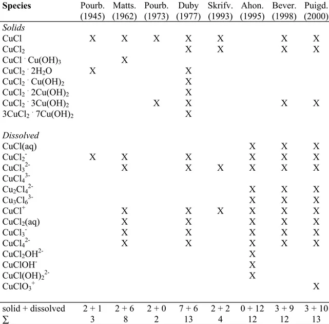
Pourbaix diagrams for the copper-chlorine system have been published by Pourbaix (1945), Duby (1977), and Beverskog and Puigdomenech (1998). The first two reported only for 25°C , while the last reported for 5-100°C . Pourbaix diagrams for the copper-chloride system have been reported by Mattsson (1962), Pourbaix (1973), Skrifvars (1993), Ahonen (1995), Nila and González (1996), and Puigdomenech and Taxén (2000). Only the two latter works presented diagrams for elevated temperatures (100°C). The concentrations of chlorine/chloride used in above studies were 0.035 to 1.7 M. The choice of species of previous works is shown in Table 1. The work of Nila and González is not considered as NH3 was included and unit copper concentration was

used.

To qualify the thermodynamic predictions of the corrosion behavior of copper in chloride solutions three different groundwaters have been experimentally tested: standard (0.0015 m Cl-), saline (0.4 m Cl-) and highly saline (1.5 m Cl-). Weight loss measurements, solution analysis, and electrochemical methods were used to check the predictions. All three thermodynamic predictions of the corrosion behavior of copper were experimentally verified, Betova et al (2003).

The aim of the present work was to calculate the thermodynamics of copper in 5 molal of chlorine. This work is an extension of a previous work with low chlorine

concentrations (0.2 and 1.5 molal), Beverskog and Puigdomenech (1998). 5 molal of chloride, which is an extreme situation that may occur in deep groundwater, have not

(6)

before been considered from thermodynamic point of view. The results from the calculations are visualized in the form of Pourbaix diagrams (potential/pH diagrams) and predominance diagrams for dissolved species. The results have been used to predict the corrosion behavior of copper in the environment for long-term repository of spent nuclear fuel. Further studies are intended to include sulfur and carbonate into the system, which will better simulate the expected repository for spent nuclear fuel. The thermodynamic calculations for copper in different aquatic environments will also be used to model the corrosion behavior of the copper canisters in the anticipated

environment of the Swedish final repository for spent nuclear fuel.

Table 1. Copper-chloride species included in previously published Pourbaix diagrams.

Species Pourb. Matts. Pourb. Duby Skrifv. Ahon. Bever. Puigd.

(1945) (1962) (1973) (1977) (1993) (1995) (1998) (2000) Solids CuCl X X X X X X X CuCl2 X X X X CuCl . Cu(OH)3 X CuCl2. 2H2O X X CuCl2. Cu(OH)2 X CuCl2. 2Cu(OH)2 X CuCl2. 3Cu(OH)2 X X X X 3CuCl2. 7Cu(OH)2 X Dissolved CuCl(aq) X X X CuCl2- X X X X X X CuCl32- X X X X X X CuCl4 3-Cu2Cl42- X X X Cu3Cl63- X X X CuCl+ X X X X X X CuCl2(aq) X X X X X CuCl3- X X X X X CuCl42- X X X X X CuCl2OH2- X CuClOH- X

(7)

2 Choice of species

It is of fundamental importance which species (solid phases, fluids, aqua complexes (ions and uncharged) and gases)) are included in the thermodynamic calculations in a given chemical system. Some species are not stable in water solutions, while others can only form at high temperatures or pressures or other extreme conditions. It is therefore necessary to critically evaluate the species, which are expected to exist in a system, before they are allowed to be the basis for the thermodynamic calculations.

Calculations based on wrong species or omitting species give misleading information on chemical equilibria. It is particularly important to include all the dissolved species in the thermodynamic calculations for Pourbaix diagrams, since they affect the size of the corrosion areas.

2.1 Chlorine - water

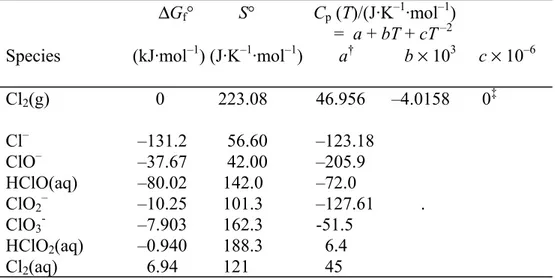
The choice of species and thermodynamic data for the chlorine-water system has been discussed elsewhere (Beverskog and Puigdomenech, 1998). The chlorate ion, ClO3-, has

been included since the previous work in accordance with the work of Puigdomenech and Taxén (2000). Eight species (seven dissolved and one gaseous) have been included in the chlorine - water system, Table 2. As seen from the Gibbs free energy values, chloride is the most stable of the chlorine species.

Table 2. Thermodynamic data at 25°C for the system chlorine-water.

∆Gf° S° Cp (T)/(J·K–1·mol–1)

= a + bT + cT –2

Species (kJ·mol–1) (J·K–1·mol–1) a† b × 103_c_{× 10}–6

Cl2(g) 0 223.08 46.956 –4.0158 0‡ Cl– –131.2 56.60 –123.18 ClO– –37.67 42.00 –205.9 HClO(aq) –80.02 142.0 –72.0 ClO2– –10.25 101.3 –127.61 . ClO3- –7.903 162.3 -51.5 HClO2(aq) –0.940 188.3 6.4 Cl2(aq) 6.94 121 45

†: For aqueous ions and complexes “a” corresponds to the standard partial molar heat capacity at 25°C , and its temperature dependence has been calculated with the revised Helgeson-Kirkham-Flowers model as described in the text.

‡: Cp° (Cl2(g), T) / (J·K–1·mol–1) = a + bT + cT –2 + dT 2 + eT-0.5, with d = 9.93 × 10−7

(8)

2.2 Copper - water

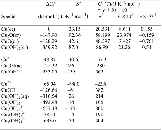
The choice of species and thermodynamical data for the copper-water system has been discussed elsewhere (Beverskog and Puigdomenech, 1995; Beverskog and

Puigdomenech, 1997). 14 copper containing species (4 solids and 10 aqueous) have been included in the calculations, Table 3.

Table 3. Thermodynamic data at 25°C for the system copper-water.

∆Gf° S° Cp (T)/(J·K–1·mol–1)

= a + bT + cT –2

Specier (kJ·mol–1) (J·K–1·mol–1) a† b × 103_c_{× 10}–6

Cu(cr) 0 33.15 20.531 8.611 0.155 Cu2O(cr) –147.90 92.36 58.199 23.974 –0.159 CuO(cr) –128.29 42.6 48.597 7.427 –0.761 Cu(OH)2(cr) –359.92 87.0 86.99 23.26 –0.54 Cu+ 48.87 40.6 57.3 CuOH(aq) –122.32 226 –280 Cu(OH)2– –333.05 –135 562 Cu2+ 65.04 –98.0 –23.8 CuOH+ –126.66 –61 382 Cu(OH)2(aq) –316.54 26 214 Cu(OH)3– –493.98 –14 105 Cu(OH)42– –657.48 –175 800 Cu2(OH)22+ –285.1 –4 190 Cu3(OH)42+ –633.0 –59 404

(9)

2.3 Copper - chlorine - water

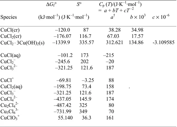
The choice of species and thermodynamic data for the system copper – chlorine – water has been discussed elsewhere (Beverskog and Puigdomenech, 1998). The mineral melanothallite, CuCl2(cr) has been included since the previous work in accordance with

the work of Puigdomenech and Taxén (2000). Thirteen species (three solids and ten dissolved) containing copper-chlorine species have been included in the aqueous system of copper-chloride, Table 4.

The complex CuClOH– was reported by Sugasaka and Fujii (1976) in 5 M NaClO4

solutions at 25°C. The existence of this species has not been verified by any other source. Furthermore, the data at 250°C by Var’yash and Rekharskiy (1981) that was explained by these authors with the formation of CuClOH– can also be modeled in a satisfactory way by assuming the formation of CuCl2– and CuCl32– only. Therefore,

CuClOH– is not included in the calculations presented here.

Table 4. Thermodynamic data at 25°C for the system

copper-chlorine-water.

∆Gf° S° Cp (T)/(J·K–1·mol–1)

= a + bT + cT –2

Species (kJ·mol–1) (J·K–1·mol–1) a† b × 103_c_{× 10}–6

CuCl(cr) –120.0 87 38.28 34.98 CuCl2(cr) –176.07 116.7 67.03 17.57 CuCl2 ⋅3Cu(OH)2(s) –1339.9 335.57 312.621 134.86 -3.109585 CuCl(aq) –101.2 173 –215 CuCl2– –245.6 202 –20 CuCl32– –321.25 121.6 187 CuCl+ –69.81 –3.25 88 CuCl2(aq) –198.75 73.4 158 . CuCl3– –321.25 121.6 187 CuCl42– –437.05 145.9 174 Cu2Cl42- –487.42 325 80 Cu3Cl63- –731.99 349 70 CuClO3+ 55.140 36.3 161

(10)

(11)

3 Thermochemical data

A critical review of published thermodynamic data has been performed for the solids and aqueous species described in previous sections. Data is usually available only for a reference temperature of 25°C in the form of standard molar Gibbs free energy of formation from the elements (∆fG°), standard molar entropy (S°), and standard molar

heat capacity (Cp°). The standard partial molar properties are used for aqueous species.

Extrapolation of these data to other temperatures is performed with the methodology described later in the “Calculations” section. Missing entropy and heat capacity values for copper species and compounds at 25°C have been estimated as described below in this section. The data selected for the calculations performed in this report are

summarized in Tables 2, 3 and 4. Values for entropy (and enthalpy) changes selected in different studies depend on the equations used for the temperature variation of Cp° for

aqueous solutes, and therefore, some of the S° values selected here differ substantially from those in other compilations, as discussed below.

Auxiliary data for chlorine, and its aqueous species, has been retrieved from the USGS report by Robie et al. (1978), the NBS compilation of Wagman et al. (1982),

CODATA’s key values by Cox et al. (1989), the NEA uranium review by Grenthe et

al. (1992), and the Cp° values given in papers by Shock and Helgeson (1988 and 1989).

3.1 Solids

The standard Gibbs free energy of formation and entropy for nantokite, CuCl(cr), is that selected by Wang et al. (1997), while the heat capacity data is that reported in

Kubaschewski et al. (1993). For atacamite (CuCl2·3Cu(OH)2(cr)) the data is that of

King et al. (1973), except for the heat capacity, which has been estimated with the methods given in Kubaschewski et al. (1993). It should be noted that the standard Gibbs free energy of formation of atacamite seems to originate from the solubility study of Näsänen and Tamminen (1949).

The soluble mineral melanothallite, CuCl2(cr), has been included since the previous

work in accordance with the work of Puigdomenech and Taxén (2000). The Cpo(T) function is from Kubaschewski et al. (1993).

(12)

3.2 Aqueous species

The thermodynamic properties of H2O(l) at 25°C recommended by CODATA (Cox et

al., 1989) have been used in this work. The temperature dependence of these properties

has been calculated with the model of Saul and Wagner (1989). The dielectric constant of water (which is needed for the revised Helgeson-Kirkham-Flowers model described below) has been obtained with the equations given by Archer and Wang (1990). The ∆Gf° value for CuCl(aq) has been obtained from the equilibrium constant reported

by Ahrland and Rawsthorne (1970) extrapolated from 5 M NaClO4 to I=0 with the

specific ion interaction equations given in Appendix D of Grenthe et al. (1992). The S° value for CuCl(aq) was obtained from the T-dependence of the equilibrium constant of formation for this complex as reported by Crerar and Barnes (1976). CuCl(aq) is a minor species which has a large uncertainty in its thermodynamic data, and does not predominate in the any of the Pourbaix diagrams presented here.

∆Gf° and S° values for CuCl2– and CuCl32– are those recommended by Wang et al.

(1997). The Cp° data has been obtained from the T-dependence of the equilibrium

constants in Var'yash (1992) for CuCl2–, while for CuCl32– a Cp° value was obtained by

analogy with the chloride complexes of silver(I) studied by Seward (1976).

∆Gf° and S° values for CuCl+ and CuCl2(aq) are those recommended by Wang et al.

(1997). Corresponding values for CuCl3– and CuCl42– are difficult to obtain because

these weak complexes are only formed at high concentrations of chloride ion. The high [Cl–_{] values result in significant changes in the activity coefficients during the}

experiments. Extrapolation of the thermodynamic data to standard conditions (zero ionic strength) will depend largely on the methodology used to estimate the effects of the changing ionic media on equilibrium constants and enthalpies of reaction.

Furthermore, the effects of changing background electrolyte concentrations and those of complex formation are mathematically highly correlated. This results in large

uncertainties associated with thermodynamic data of weak complexes at standard conditions. In general, strong physical evidence from a variety of experimental techniques is often required to establish un-equivocally the existence and strength of

(13)

Cu2+ + Cl– →_←_CuCl+ _∆H_r_{° = 8.4 (Wang et al., 1997)}

Cu2+ + 2 Cl– →_←_CuCl₂_(aq) _∆H_r_{° = 23} _"

-Cu2+ + 3 Cl– →_←_CuCl₃– _∆H_r_{° = 30} _Estimated

Cu2+ + 4 Cl– →_←_CuCl₄2– _∆H_r_{° = 40} _Estimated

It should be pointed out that the relatively large uncertainties in the standard values for CuCl3– and CuCl42– do not affect the results of the present study, because of the

restricted range of chloride concentrations it involves.

The Cp° data for all four chloride complexes of Cu(II) has been obtained by analogy

with the zinc(II) system using the ∆rCp° values reported by Ruaya and Seward (1986).

The data for the copper(II) chlorate ion, CuClO3-, is selected from the work of

(14)

(15)

4 Calculations

The methods and assumptions to calculate equilibrium diagrams have been described elsewhere (Beverskog and Puigdomenech, 1995 and 1996). The technique to draw Pourbaix diagrams has also been presented by Beverskog and Puigdomenech (1995). Pourbaix diagrams have been drawn with computer software (Puigdomenech, 1983) using the chemical compositions calculated with the SOLGASWATER algorithm (Eriksson, 1979), which obtains the chemical composition of systems with an aqueous solution and several possible solid compounds by finding the minimum of the Gibbs free energy of the system.

The ionic strength for the calculations corresponding to each coordinate in the diagrams has been calculated iteratively from the electro neutrality condition: on acid solutions a hypothetical anion has been ideally added to keep the solutions neutral and on alkaline solutions a cation has been added. These hypothetical components have been taken into account when calculating the value of the ionic strength.

The values for the activity coefficient, γi, of a given aqueous ion, i, have been

approximated with a function of the ionic strength and the temperature: log γi = – zi2 A √I / (1 + B å I ) – log (1+0.0180153 I) + b I

where I is the ionic strength, A, B, and b are temperature-dependent parameters, zi is the

electrical charge of the species i, and å is a “distance of closest approach”, which in this case is taken equal to that of NaCl (3.72 × 10–10_{m). This equation is a slight}

modification of the model by Helgeson et al., (see Eqs. 121, 165-167, 297, and 298 in Helgeson et al. (1981); and Eqs. 22 and 23 in Oelkers and Helgeson (1990)). The values of A, B, and b at a few temperatures are:

T / °C p / bar A B b 25 1.000 0.509 0.328 0.064 100 1.013 0.600 0.342 0.076 150 4.76 0.690 0.353 0.065 200 15.5 0.810 0.367 0.046 250 39.7 0.979 0.379 0.017 300 85.8 1.256 0.397 –0.029

For neutral aqueous solutions, it has been approximated that their activity coefficients are unity at all values of ionic strength and temperature. This would have negligible effects on the calculated Pourbaix diagrams.

(16)

The effect of the activity corrections for higher ion strength was observable on the diagrams compared to those calculated at I=0. For example, the stability of the solid phase CuCl2. 3Cu(OH)2 is reduced in the corrected version, and the predominance area

of the uncharged complex Cu(OH)2(aq) is also affected.

Calculations to draw the diagrams presented in this work have been performed for five temperatures in the interval 5-100°C (5, 25, 50, 80, and 100), which covers adequately the temperature range which copper canisters will experience in the expected

environment of the Swedish final repository for spent nuclear fuel. Calculations have been performed at two total concentrations of dissolved copper species 10-4_{and 10}-6

molal (mol/kg of water) at a chloride concentration of 5 molal. Because they are temperature-independent, molal concentration units are used in the calculations.

The parallel sloping dashed lines in the Pourbaix diagrams given in the Appendix limit the stability area of water at atmospheric pressure of gaseous species. The upper line represents the oxygen equilibrium line (O2(g)/H2O(l)) and potentials above this line will

oxidize water with oxygen evolution. The lower line represents the hydrogen line (H+_/H

2(g)) and potentials below this line will result in hydrogen evolution.

All values of pH given in this work are values at the specified temperature. The temperature dependence for the ion product of water,

H2O(l) ←→ H+ + OH–

changes the neutral pH value of pure water with the temperature (neutral environment = 1/2 pKw,T). To facilitate reading the Pourbaix diagrams in the Appendix, the

anticipated redox potentials of –300 to –400 mVSHE at 25°C and a pH25_°Cof 7-9 for the

(17)

5 Result and discussion

The Pourbaix diagrams for copper – chlorine and copper – chloride are equivalent. This is due to that only one chlorine species is stable in the stability area of water, namely chloride. Therefore Pourbaix diagrams for copper – chlorine can be used to discuss the copper – chloride system.

5.1 General behavior

Two general remarks can be concluded regarding the temperature and concentration dependence of the diagrams. Firstly, temperature affects the different stability areas of immunity, passivity and corrosion. The immunity area (stability of the metal itself) decreases with increasing temperature. The passivity area (solid compounds) is almost temperature independent. With increasing temperature the corrosion area at acidic pH changes due to a slight decrease of the passivity area and a decrease of the immunity area, while the corrosion area at alkaline pH increases (it is shifted to lower pH values). The reason for this behavior is related to the temperature dependence of the ion product of water. Secondly, the concentration of dissolved metallic species also changes the different stability areas. The immunity and passivity areas increase with increasing concentration at increasing temperature, while the corrosion areas decrease.

The results from the thermodynamic calculations for the aqueous system of chlorine and copper-chlorine are summarized in Pourbaix diagrams with two concentrations of dissolved copper species (10-4_{and 10}-6_{m), but constant chlorine content (5 m).}

The Pourbaix diagrams for the system chlorine-water at the total concentration of 5 molal chlorine are shown in figs. 1A-E. The diagrams show that the only stable species of chlorine in aqueous solutions is chloride. At potentials above the stability area of water (between the dotted parallel sloping lines) only Cl2(g) and ClO3- forms.

The Pourbaix diagrams for chlorine show that the only stable chlorine species in

aqueous solutions is the chloride ion. Therefore, Pourbaix diagrams for a metal-chlorine system can be used to predict the effect of chloride in that metal system.

The Pourbaix diagrams for copper at [Cu(aq)]tot = 10-4 m and [Cl(aq)]tot = 5 m are

shown in figs. 2A-E. The presence of chlorine decreases both the immunity area of copper and the passivity area of Cu2O and CuO calculated in Beverskog and

Puigdomenech (1995) due to the aqueous complex CuCl32-. The complex predominates

also at 1.5 m, but not at 0.2 m where CuCl2- predominates (Beverskog and

Puigdomenech, 1998). The corrosion areas increase as a result of the decrease in immunity and passivity areas. This is due to the high affinity of copper for chloride, as the latter is a strong complex former. The corrosion area of CuCl32- is large, from

strongly acidic to highly alkaline solutions. The temperature dependence of the

predominance area of CuCl32- increases with increasing temperature. CuCl32- oxidizes in

(18)

Elemental copper passivates only in highly alkaline solutions by formation of Cu2O.

Increasing temperatures decreases the stability area of Cu2O. Still higher pH corrodes

elemental copper by formation of the second hydrolysis complex of copper(I), Cu(OH)2-.

Copper(I) oxide oxidizes at higher potentials (in the middle of the stability area of water) to copper(II) oxide, CuO. The latter has a larger pH interval where it is stable. Increasing pH dissolves CuO by formation of Cu(OH)42-. Decreasing pH can transform

CuO to CuCl2.3Cu(OH)2, which can dissolve at still lower pH by formation of

CuCl2(aq).

The predominance diagrams for copper species at [Cu(aq)]tot = 10-4 m and [Cl(aq)]tot =

5 m are shown in figs. 3A-E. The predominating dissolved species in equilibria with elemental copper in strongly acidic to highly alkaline solutions is CuCl32- not Cu+. At

still higher pH elemental copper is in equilibria with the second hydrolysis step of copper(I), Cu(OH)2-. The dissolved species in equilibria with copper(I) oxide is either

CuCl32- or Cu(OH)2-, dependent of pH. The dissolved species in equilibria with

copper(II) oxide is Cu2+_{at T > 50}_{°C , CuCl}

32-, Cu(OH)2(aq), Cu(OH)3-, or Cu(OH)42-,

dependent of potential and pH. The dissolved species in equilibria with

CuCl2.3Cu(OH)2 is CuCl32-, CuCl2(aq), or Cu(OH)2(aq), dependent of potential and pH.

The Pourbaix diagrams for copper at [Cu(aq)]tot = 10-6 m and [Cl(aq)]tot = 5 m are

shown in figs. 4A-E. The lower copper concentration decreases the immunity and passivity areas, while the corrosion areas increase. Copper dissolves (corrodes) and forms CuCl32- in acidic to alkaline solutions, and Cu(OH)2- forms in highly alkaline

solutions. The corrosion region between the between the immunity and passivity region is due higher stability of CuCl32- and Cu(OH)2- compared to Cu2O. Copper(I) oxide is

not stable in this environment and therefore a corrosion region exists between the immunity and passivity areas. However, copper can passivates, and form

CuCl2.3Cu(OH)2 or CuO, at potentials around the oxygen line. The immunity and

passivity areas decrease with increasing temperature, while the corrosion areas increase. The presence of chlorine decreases both the immunity area of copper and the passivity area of Cu2O calculated in Beverskog and Puigdomenech (1995) due to the aqueous

complex CuCl32-. The complex predominates also at 1.5 m, but not at 0.2 m.

The predominance diagrams for dissolved copper species at [Cu(aq)]tot = 10-6 m and

(19)

5.2 Corrosion of copper at repository potentials, pH and

temperatures

The environment around the copper canisters in the deep repository for spent nuclear fuel has an anticipated redox potential range of –300 to –400 mVSHE, pH25_°C 7 - 9, and a

temperature around 80°C .

Corrosion of copper in 5 molal chloride solution at repository potentials, pH and temperatures will be discussed for four different scenarios. The corrosion behavior of copper is predicted from the thermodynamic calculations. The main physiochemical parameters in the deep repository can be summarized as:

• Initial phase: oxidizing conditions temperature 80-100°C short phase

• Main phase: anoxic conditions temperature: 80°C • Glacial phase: oxidizing conditions

temperature: 5°C • Cooling phase: anoxic conditions

temperature: 80-5°C

Initial Phase

The initial phase is oxidizing due to residual oxygen after closing the repository and the temperature is in the interval of 80-100°C. The residual oxygen will be consumed (cathodic reaction) in the corrosion process of the copper canisters (anodic reaction). Copper corrodes in this environment, due to high stability of the copper(I) chloride complex, CuCl32-. The corrosion area is large and corrosion will take place as long as

pH is < 11 at a copper concentration of 10-4 m. The corrosion area at [Cu(aq)]tot = 10-6

m, which is the conventional definition for corrosion, exists in the whole investigated pH range, as no solid compound forms.

The degree of oxidizing conditions affect the redox potential, but it is unlikely that the initial condition will raise the potential into the passivity area of CuO. Therefore, corrosion of copper will occur during the initial phase.

(20)

Main phase

The main phase is under anoxic conditions and the temperature ∼ 80°C . The

conventional definition for corrosion (10-6 m), predicts corrosion of copper and this is independent of pH. In the case of a higher concentration of dissolved copper (0.1 mmolal) the lower end of the estimated potential range, the potential will fall in the immunity region. Then no corrosion per definition can occur. In the upper part of the potential range corrosion will occur.

Glacial phase

During a glacial phase cold oxygenated water may enter the repository. The temperature will be ∼ 5°C and the oxygen content can be high. The potential-pH box in the diagrams will be lifted up into the corrosion area. Corrosion of copper will occur, and the

corrosion rate can be high. However, the low temperature decreases the kinetics for the electrochemical reactions, which means reduced reaction (corrosion) rate. This situation can easily be experimentally examined with an air saturated (8 ppm dissolved oxygen at 25°C ) solution at 5°C.

Cooling phase

During the cooling phase the temperature will decrease and finally end at the

temperature of non-heat effected ground water, ~ 5°C . The redox conditions will be anoxic. Copper will corrode at 10-6 m at 80 - 50°C , but not at 25 and 5°C , as the potential will be in the immunity area.

5.3 Corrosion of copper canisters in a deep repository

Two barriers will surround the copper canisters in the long-term deep repository for spent nuclear fuel. The first barrier is of compacted bentonite clay, which surrounds the copper canisters and will fill the cave in the bedrock. The second barrier is the granite bedrock in which the repository cave is built. The two barriers affect the transport of eventual radioactive species from the spent nuclear fuel. These barriers also affect the corrosion behavior of the copper canisters. The outer barrier, the granite bedrock, will

(21)

oxidizing agents and aggressive anions coming from outside the repository as well as the outward transport of dissolved corrosion products of copper are affected.

The space between the copper canisters and the surrounding bentonite clay is assumed to be a few mm to 2 cm. This space will be filled by ground water. The swelled

bentonite clay with its limited transport rates and the copper canisters can be considered as a “closed” system from the macroscopic point of view. This “closed” system strongly affects the corrosion behavior of the copper canisters.

Inward diffusion

The initially high concentration of oxygen at the moment of closing the repository will be consumed in a relatively short time. Additional oxidizing agents must be transported through the barrier of bentonite clay. (Assuming that the thickness of the copper and carbon steel is sufficient to eliminate radiolysis of the water in the gap between copper canisters and the clay). Oxygen will also be consumed by different redox reactions in the clay. This means that the concentration of oxygen in the ground water outside the copper canisters will decrease and thereby also the corrosion potential will decrease. In time the corrosion potential will fall in the immunity area of copper, see Beverskog and Puigdomenech (1995). The corrosion of copper will thereby stop as the metal is

cathodically protected.

Outward diffusion

The outward diffusion of dissolved corrosion products has also transport restrictions through the bentonite clay. This means that the concentration of dissolved copper species will increase in the aqueous solution between the bentonite clay and copper canisters. The increase will continue until an equilibria is achived between the dissolved speices and the copper surface. Increasing levels of dissolved species increases the size of the immunity area in the Pourbaix diagrams. The increasing concentration of

dissolved species changes the equilibria Cu(cr) / CuCl32-(aq) to higher potentials

(anodic direction). The increase will continue until the corrosion potential is situated in the immunity area of copper. The corrosion of copper will thereby stop, as the metal is cathodically protected.

The phenomena of inward diffusion is not isolated from the outward diffusion

phenomena. Both will occur simultaneously in parallel to each other. Both phenomena will cause the corrosion potential to end up in the immunity area of copper, where the metal itself is the thermodynamically stable species. With other words, one process is forcing the potential in the cathodic (negative) direction, while the other process expands the immunity area. The result is that the corrosion potential of copper will fall in the immunity area and corrosion will stop.

There will be a concentration gradient of the dissolved copper species in the bentonite clay due to the limited diffusion rate of copper. The amount of dissolved copper species can also form clusters, which further reduces the transport rate through the bentonite

(22)

clay. These clusters can grow further and form colloids. The size of the colloids will further restrict the diffusion rate of the formed colloids. This may lead to blocking of the pores and thereby causing further decrease of the outward diffusion rate. However, blocking the pores with colloids in the clay will also decrease the inward diffusion of oxidizing agents (as well as aggressive anions). This will further decrease the corrosion potential and force it into the immunity region.

Oxygen has a measurable diffusion rate through bentonite. The concentration of oxygen at –300 to –400 mVSHE is relatively low. Oxygen will also be consumed by pyrite in the

bentonite clay. This means that the concentration of oxygen will be very low at the surface of the copper canisters.

The outward diffusion of dissolved copper(I) complexes will create a concentration gradient in the bentonite clay, with the highest concentration at the inner interface, clay / gap water. The high concentration can form polynucleous complexes such as Cu2Cl4

2-and Cu3Cl63-. These complexes will form clusters, and the clusters can form larger

aggregates such as colloids. The colloids can form a gel like structure in the diffusion paths and blocking transport trough the pores, and thereby sterically hinder further outward diffusion of dissolved complexes. This means an increase of dissolved copper concentration in the gap until the growth of the immunity area cause the corrosion potential to fall inside it. Thereby the corrosion will stop.

The formed barrier of a gel like structure of copper(I) complexes, also hinders the inward diffusion of oxygen. Complexes at the outer interface of the gel will oxidize to CuCl2(aq). A redox couple will be formed between one and two valent copper

complexes, which will establish a certain redox potential.

If oxygen is enriched at the outer interface of the gel like structure, a concentration gradient of oxygen will be formed. This will create a driving force of backward diffusion of oxygen to equilibriate the conditions of oxygen. This means that the concentration of oxygen will decrease to certain value. This will further decrease the corrosion potential of copper and force it into the immunity area.

Concerning a “closed” system where the corrosion of copper stops is the same for the initial, main and cooling phases. In the glacial phase, the situation is also relevant as long as no cracks are formed in the bentonite clay. However, with the heavy mass of a

thick layer of ice it is likely that macro cracks will form in the bentonite clay. Thereby,

(23)

6 Conclusions

The results of the thermodynamic calculations for copper in 5 molal chloride can be summarized as:

• Chloride reduces the immunity and passivity areas of copper. • Copper corrodes in 5 m Cl-_{by formation of CuCl}

32- in acid and alkaline solutions.

• CuCl32- is oxidized at higher potentials to CuCl2(aq).

• CuCl2(aq) can at increasing potentials form CuCl+, Cu2+ or CuClO3+, while the latter

only predominates at 5-50°C .

• Copper can passivates by formation of Cu2O(cr), CuO(cr), or CuCl2. 3Cu(OH)2(s).

• Cu2O(cr) does not form at [Cu(aq)]tot = 10-6 m, which results in a corrosion area

between the immunity and passivity regions.

• CuCl2. 3Cu(OH)2(s) does not form at [Cu(aq)]tot = 10-6 m at 80 and 100°C due to

higher stability of CuCl2(aq).

• Copper at repository potentials and pH corrodes at 100°C at [Cu(aq)]tot = 10-4 m and

at 80 and 100°C at [Cu(aq)]tot = 10-6 m.

• Copper at repository potentials and pH can corrode at 80°C at [Cu(aq)]tot = 10-4 m

and at 50°C at [Cu(aq)]tot = 10-6 m.

• The bentonite clay and the copper canisters can be considered as a “closed” system from macroscopic point of view.

• The clay barrier limits both inward diffusion of oxygen and aggressive anions as well as outward diffusion of dissolved corrosion products of copper.

• Both diffusion processes will cause the corrosion potential to fall into the immunity area of copper in the Pourbaix diagram.

• Corrosion of the copper canisters will thereby automatically stop. This means that the engineered system of clay and copper has an inbuilt auto-stop of corrosion. However, this is only valid if no macro cracks occur in the clay.

• The auto-stop is valid during the initial, main and cooling phases. However, during a glacial period the weight of the ice may cause macro cracks and open the “closed” system, and thereby cause accelerated corrosion.

(24)

(25)

Acknowledgments

Thank is due to Christina Lilja for her patience and encouragement and Dr. I. Puigdomenech for stimulating discussions.

(26)

(27)

References

Ahonen, L. (1995). Chemical stability of copper canisters in deep repository. Report YJT 95-19, Nuclear Waste Commission of Finnish Power Companies.

Ahrland, S. and Rawsthorne, J. (1970). The stability of metal halide complexes in aqueous solution. VII. The chloride complexes of copper(I). Acta Chem. Scand., 24, 157-172.

Archer, D.G. and Wang, P. (1990). The dielectric constant of water and Debye-Hückel limiting law slopes, J. Phys. Chem. Ref. Data, 19, 371-411.

Betova, I., Beverskog, B., Bojinov, M., Kinnunen, P., Mäkelä, K., Pettersson, S.-O., and Saario, T. (2003). Corrosion of copper in simulated nuclear waste repository

conditions. Electrochem. Solid-State Let, 6, B19.

Beverskog, B. and Puigdomenech, I. (1995). SITE-94. Revised Pourbaix diagrams for copper at 5-150°C, SKI Report 95:73, Swedish Nuclear Power Inspectorate, Stockholm, Sweden.

Beverskog, B. and Puigdomenech, I. (1996). Revised Pourbaix diagrams for iron at 25– 300°C, Corrosion Sci., 38, 2121-2135.

Beverskog, B. and Puigdomenech, I. (1997). Revised Pourbaix diagrams for copper at 25 to 300°C, J. Electrochem. Soc., 144, 3476-3483.

Beverskog, B. and Puigdomenech, I. (1998). SITE-94. Pourbaix diagrams the system copper chlorine at 5-100°C, SKI Report 98:19, Swedish Nuclear Power Inspectorate, Stockholm, Sweden.

Cox, J. D., Wagman, D. D., and Medvedev, V. A. (1989). CODATA key values for

thermodynamics. Hemisphere Publ. Co., New York.

Crerar, D. A., and Barnes, H. L. (1976). Ore solution chemistry V. Solubilities of chalcopyrite and chalcocite assemblages in hydrothermal solution at 200° to 350°C,

Econ. Geol., 71, 772-794.

Duby, P. (1977). The Thermodynamic Properties of Aqueous Inorganic Copper systems. INCRA Monograph IV. The Metallurgy of Copper. Int. Copper Res. Ass..

Eriksson, G. (1979). An algorithm for the computation of aqueous multicomponent, multiphase equilibria, Anal. Chim. Acta, 112, 375-383.

(28)

Grenthe, I., Fuger, J., Konings, R. J. M., Lemire, R. J., Muller, A. B.,

Nguyen-Trung, C., and Wanner, H. (1992). Chemical thermodynamics of uranium, Elsevier Sci. Publ., Amsterdam.

Helgeson H.C., Kirkham, D.H. and Flowers, G.C. (1981). Theoretical prediction of the thermodynamic behaviour of aqueous electrolytes at high pressures and

temperatures: IV. Calculation of activity coefficients, osmotic coefficients, and apparent molal and standard and relative partial molal properties to 600°C and 5 kb,

Amer. Jour. Sci., 281, 1249-1516.

King, E. G., Mah, A. D. and Pankratz, L. B. (1973). Thermodynamic properties of

copper and its inorganic compounds, The International Copper Research Association

(INCRA), New York.

Kubaschewski, O., Alcock, C. B. and Spencer, P. J. (1993). Materials thermochemistry. Pergamon Press, Oxford, 6th edition.

Mattsson, E. (1962) Potential-pH diagram för korrosionsstudier. Med

beräkningsexempel avseende systemet Cu-Cl-H2O, Svensk Kemisk Tidskrift, 74,

76-88.

Näsänen, R. and Tamminen, V. (1949) The equilibria of cupric hydroxysalts in mixed aqueous solutions of cupric and alkali salts at 25°, J. Am. Chem. Soc., 71, 1994– 1998.

Nila, C. and González, I. (1996). Thermodynamics of Cu-H2SO4-Cl–-H2O and

Cu-NH4Cl-H2O based on predominance-existence diagrams and Pourbaix-type

diagrams, Hydrometallurgy, 42, 63-82.

Oelkers, E.H. and Helgeson, H.C. (1990) Triple-ion anions and polynuclear complexing in supercritical electrolyte solutions, Geochim. Cosmochim. Acta, 54, 727-738. Pourbaix, M. (1945). Thermodynamique des Solutions Aqueuses Diluées.

(29)

Puigdomenech, I. and Taxén, C. (2000). Thermodynamic data for copper: implications for the corrosion of copper under repository conditions, SKB Report TR-00-13. Ramette, R. W. (1986). Copper(II) complexes with chloride ion, Inorg. Chem., 25,

2481–2482.

Robie, R. A., Hemingway, B. S. and Fisher, J. R. (1978). Thermodynamic properties of minerals and related substances at 298.15 K and 1 bar (105 Pascals) pressure and at higher temperatures, USGS Bull. 1452.

Ruaya, J. R. and Seward, T. M. (1986). The stability of chlorozinc(II) complexes in hydrothermal solutions up to 350°C, Geochim. Cosmochim. Acta, 50, 651–661. Saul, A. and Wagner, W. (1989). A fundamental equation for water covering the range

from the melting line to 1273 K at pressures up to 25 000 MPa, J. Phys. Chem. Ref.

Data, 18, 1537–1564.

Seward, T. M. (1976). The stability of chloride complexes of silver in hydrothermal solutions up to 350°C, Geochim. Cosmochim. Acta, 40, 1329–1341.

Shock, E. L. and Helgeson, H. C. (1988). Calculation of the thermodynamic and transport properties of aqueous species at high pressures and temperatures:

correlation algorithms for ionic species and equation of state predictions to 5 kb and 1000°C, Geochim. Cosmochim. Acta, 52, 2009–2036. Errata: 53 (1989) 215.

Shock, E. L., Helgeson, H. C., and Sverjensky, D. A. (1989). Calculation of the thermodynamic and transport properties of aqueous species at high pressures and temperatures: standard partial molal properties of inorganic neutral species,

Geochim. Cosmochim. Acta, 53, 2157–2183.

Skrifvars, B. (1993). Metal Pourbaix diagrams in complexing environments. The use of thermodynamic stability diagrams for predicting corrosion behavoiur of metals,

Progress in Understanding and Prevention of Corrosion, Vol.1, Barcelona, Spain,

July 1993, p. 437-446.

Sugasaka, K. and Fujii, A. (1976). A spectrophotometric study of copper(I)

chlorocomplexes in aqueous 5 M Na(Cl,ClO4) solutions, Bull. Chem. Soc. Japan, 49,

82-86.

Var'yash, L. N. (1992) Cu(I) complexing in NaCl solutions at 300 and 350°C, Geochem.

(30)

Var'yash, L. N. and Rekharskiy, V. I. (1981). Behaviour of Cu(I) in chloride solutions,

Geochem. Int., 18, 61-67.

Wagman, D. D., Evans, W. H., Parker, V. B., Schumm, R. H., Halow, I., Bailey, S. M., Churney, K. L. and Nuttall, R. L. (1982). The NBS tables of chemical

thermodynamic properties: Selected values for inorganic and C1 and C2 organic

_{5 C}o

Potential (V )

Potential (V )

SHE Figure 4B

(49)

Cu2+ Cu(OH)42- Cu(OH)2- CuCl32-CuCl + CuCl2(aq) CuClO3+ CuO(cr) Cu(cr) CuCl2.3Cu(OH)2(s)