2010:22 Research and Development Program in Reactor Diagnostics and Monitoring with Neutron Noise Methods, Stage 16

(1)

Research

2010:22

_{Research and Development Program}

in Reactor Diagnostics and Monitoring

with Neutron Noise Methods, Stage 16

Authors: Imre Pázsit

Victor Dykin Anders Jonsson Christophe Demazière

(2)

(3)

Title: Research and Development Program in Reactor Diagnostics and Monitoring with Neutron Noise Methods, Stage 16

Report number: 2010:22

Author: Imre Pázsit, Victor Dykin, Anders Jonsson and Christophe Demazière

Chalmers University of Technology, Department of Nuclear Engineering, SE-412 96 Göteborg

Date: December 2010

This report concerns a study which has been conducted for the Swedish Radiation Safety Authority, SSM. The conclusions and viewpoints presented in the report are those of the authors and do not necessarily coincide with those of the SSM

SSM Perspective Background

This report constitutes Stage 16 of a long-term research and develop-ment program concerning the developdevelop-ment of diagnostics and monito-ring methods for nuclear reactors.

Results up to Stage 15 were reported in SKI and SSM reports, as listed below and in the Summary. The results have also been published in international journals and have been included in both licentiate- and doctor’s degrees.

Objectives of the project

The objective of the research program is to contribute to the strate-gic research goal of competence and research capacity by building up competence within the Department of Nuclear Engineering at Chalmers University of Technology regarding reactor physics, reactor dynamics and noise diagnostics. The purpose is also to contribute to the research goal of giving a basis for SSM’s supervision by developing methods for identification and localization of perturbations in reactor cores.

Results

The program executed in Stage 16 consists of the following three parts: • An overview of the present status of experience with BWR stability; • An investigation of the significance of the properties of the noise

source for BWR instability;

• Study of the dynamics of molten salt systems: construction of the adjoint and calculating the space dependent noise induced by propagating perturbations in the fuel;

• A specific study of some novel methods of analysis of non-linear and non-stationay processes.

Project information

Responsible at SSM has been Ninos Garis. SSM reference: SSM 2009/2093

Previous SKI reports: 95:14 (1995), 96:50 (1996), 97:31 (1997), 98:25 (1998), 99:33 (1999), 00:28 (2000), 01:27 (2001), 2003:08 (2003), 2003:30 (2003), 2004:57 (2004), 2006:34 (2006), 2008:39 (2008), Previous SSM reports: 2009:38 (2009)

(4)

(5)

Summary

This report gives an account of the work performed by the Department of Nuclear Engineering, Chalmers University of Technology, in the frame of a research contract with the Swedish Radiation Safety Authority (SSM), contract No. SSM 2009/2093. The present report is based on work performed by Imre Pázsit, Victor Dykin, Anders Jonsson and Christophe Demazière, with Imre Pázsit being the project leader.

This report describes the results obtained during Stage 16 of a long-term research and development program concerning the development of diagnostics and monitoring methods for nuclear reactors. The long-term goals are elaborated in more detail in e.g. the Final Reports of Stage 1 and 2 (SKI Report 95:14 and 96:50, Pázsit et al. 1995, 1996). Results up to Stage 15 were reported in (Pázsit et al. 1995, 1996, 1997, 1998, 1999, 2000, 2001, 2003a, 2003b; Demazière et al, 2004; Sunde et al, 2006; Pázsit et al. 2008, 2009). A brief proposal for the continuation of this program in Stage 17 is also given at the end of the report.

The program executed in Stage 16 consists of four parts as follows: An overview of the present status of experience with BWR stability;

An investigation of the significance of the properties of the noise source for BWR instability;

Study of the dynamics of molten salt systems: construction of the adjoint and calculating the space dependent noise induced by propagating perturbations in the fuel;

A specific study of some novel methods of analysis of non-linear and non-stationary processes.

The work performed in each part is summarized below.

1. An overview of the present status of experience with BWR stability

This section gives an overview of the main trends in BWR stability analysis and monitoring for the past decade. The major line of development in this period has been the recognition that different types of neutronic and thermal hydraulic oscillations may occur (global, regional and local or channel-type), with different generation mechanisms, impact on core safety, and monitoring tools and needs. In particular, when any two of these types can occur simultaneously, it is important to separate the different components, otherwise the margin to instability can be misjudged severely. Any procedure aiming at stability monitoring should be able to detect the presence of simultaneous oscillations, as well as to classify their type and stability properties separately. In this respect global and regional type instabilities are a larger potential operational problem than local oscillations, because their amplitude can grow unbounded. Local oscillations are purely thermal hydraulics driven, and it is not so much the stability properties than the localisation which is of concern.

This section starts with a description of the three main oscillation types and their properties. The concept of the most commonly used stability parameter, the decay ratio,

(8)

is described. The properties of simultaneous oscillations and the resulting apparent decay ratio obtained without separation of the components are discussed. The methods elaborated to separate the global and regional oscillations are described in detail. The noise simulator, developed at the department, is used to reconstruct some of the observed properties, such as the space dependence of the decay ratio in case of simultaneous oscillations of two different types. The localisation of a local channel-type instability is also described and its concrete application to the case of the Forsmark local instability is demonstrated.

2. An investigation of the significance of the properties of the noise source for BWR instability

In simple models used to interpret the stability properties of boiling water reactors it is assumed that the power or flux oscillations in the core can be described as the response of a damped linear oscillator, driven by a white noise driving force. Such a model proves useful in understanding the path to instability, especially the interplay of several different oscillation modes (global, regional, local). In the model it is assumed that the stability properties, extracted from the measured oscillations, are determined purely by the system transfer properties, due to the fact that the driving force has a spectrum which is constant in frequency.

However, from other studies of BWR in-core noise, it is known that the reactivity perturbation corresponding to the propagating character of two-phase flow has a characteristic autospectrum which shows a periodic peak and sink structure, i.e. deviates markedly from white noise. In that case, the frequency properties, or the autocorrelation function of the measured detector signals, are influenced not only by the system transfer properties, but also by those of the driving force. Estimating the decay ratio with the assumption of white driving force can lead to erroneous results.

The influence of the ―coloured‖ character of the driving force, as represented by the reactivity perturbation of propagating density fluctuations of the two-phase flow, on the estimation of the decay ratio is investigated. The autocorrelation function of the system response with such a coloured driving force is calculated analytically. Cases when the driving force has a peak or a sink at the system resonance frequency are investigated quantitatively. The results show that in the case of propagating perturbations the structure of the driving force is relatively smooth at the system resonance, and no significant error is made in the estimation of the decay ratio assuming a white noise driving force.

3. Study of the dynamics of molten salt systems: construction of the adjoint and calculating the space dependent noise induced by propagating perturbations in the fuel

In previous reports, starting with Stage 13, a simple one-dimensional model with propagating fuel properties was set up and studied as a model of a molten salt reactor. First the solution of the static eigenvalue equation was given first by expansions into eigenfunctions of a corresponding traditional reactor. The neutron noise, induced by propagating perturbations, was calculated in the point kinetic approximation, by using a simplified empirical model of the zero reactor transfer function G₀( ), suggested in the

(9)

literature. It was also noticed that the derivation of the point kinetic approximation with the flux factorisation technique is hindered by the fact that the one-group diffusion equations for a reactor with moving fuel are not self-adjoint.

In Stage 15, the solution of the space-dependent noise problem was started with the calculation of the Green’s function of the problem. The space-dependent problem was solved for the case of infinite fuel velocity, with a new technique which separates out a singular and a non-singular term in the solution, similarly to the method of eliminating the uncollided flux in transport problems.

In the present Stage, first the adjoint equations of the one-group diffusion theory are derived for reactors with moving fuel. The adjoint property of the suggested form is proven both for the differential form of the coupled neutron-precursor equations, and for the integro-differential form, obtained after eliminating the delayed neutron precursors. Then the Green’s function of the reactor is calculated for finite fuel velocities, with the employment of a method, suggested in the previous Stage for the solution for infinite fuel velocities. The space and frequency dependence of the Green’s function is investigated. Finally, the space-dependent noise, induced by propagating perturbations, are calculated and discussed. It is shown that with increasing fuel velocity, the behaviour of a given system at a given frequency tends to be more and more point kinetic, in accordance with the results for infinite fuel velocity, found in the previous Stage.

4. A specific study of some novel methods of analysis of linear and non-stationary processes

New methods have been developed lately which are particularly useful to analyse non-stationary processes in order to make a diagnosis of the state of the system. Some of the development has been achieved primarily in biology and medicine, for the analysis of ECG (heart beat) and EEG (brain activity) signals and to detect beginning and developed diseases. Some of these methods were transferred even to the diagnostics of process signals in power plants. The purpose of this pilot study is to start exploring the application of such methods in reactor diagnostics.

One such method refers to the analysis of quasi-periodic signals, such as human ECG signals. Instead of analysing the raw signal, a secondary time series is derived from the original signal, which consists of the sequence of beat-to-beat (also called ―interbeat‖) time intervals. This derived sequence is apparently random, but it contains a substantial information on the status of the system. This information can be extracted either from the topology of the three dimensional vectors, formed from triplets of consecutive values of the interbeat intervals, of from the fractal dimension of the data series, or by some other intelligent identification method.

In this Stage the method of peak-to-peak interval analysis is tested on measurements of BWR instability. The time series represented by the peak-to-peak time intervals of the signal variation around the instability frequency 0.5 Hz is analysed. First a method was developed for the extraction of the peak-to-peak series, then the topology of the three-dimensional vectors, formed from data triplets, was investigated. A different behaviour was found for the cases of a stable and an unstable state of the core, although the information content was rather obvious. Some new algorithmic identification methods,

(10)

such as Principal Component Analysis (PCA) and Singular Value Decomposition (SVD), were also tested on the data vectors, but these yielded no further information. These studies will be continued with e.g. using higher dimensional data sets, to explore their potential in BWR stability analysis.

(11)

Sammanfattning

Denna rapport redovisar det arbete som utförts inom ramen för ett forskningskontrakt mellan Avdelningen för Nukleär Teknik, Chalmers tekniska högskola, och Strålsäkerhetsmyndigheten (SSM), kontrakt Nr. SSM 2009/2093. Rapporten är baserad på arbetsinsatser av Imre Pázsit, Victor Dykin, Anders Jonsson och Christophe Demazière, med Imre Pázsit som projektledare.

Rapporten beskriver de resultat som erhållits i etapp 16 av ett långsiktigt forsknings- och utvecklingsprogram angående utveckling av diagnostik och övervakningsmetoder för kärnkraftsreaktorer. De långsiktiga målen har utarbetats noggrannare i slut-rapporterna för etapp 1 och 2 (SKI Rapport 95:14 och 96:50, Pázsit et al. 1995, 1996). Uppnådda resultat fram till och med etapp 15 har redovisats i referenserna (Pázsit et al. 1995, 1996, 1997, 1998, 1999, 2000, 2001, 2003a, 2003b; Demazière et al, 2004; Sunde et al, 2006; och Pázsit et al. 2008, 2009). Ett kortfattat förslag till fortsättning av pro-grammet i etapp 17 redovisas i slutet av rapporten.

Det utförda forskningsarbetet i etapp 16 består av följande fyra olika delar. Sammanställning av kunskapsläget för BWR-instabilitet;

Undersökning av betydelsen av bruskällan i samband med BWR-instabilitet;

Fortsatta studier av neutronkinetik, dynamik och neutronbrus i reaktorer med flytande bränsle (MSR);

Undersökning och tillämpning av ―intelligent computing‖ metoder. Arbetet med varje del sammanfattas nedan.

1. Sammanställning av kunskapsläget för BWR-instabilitet

Denna del ger en överblick av de huvudsakliga trenderna i stabilitetsanalys och över-vakning av BWR-reaktorer under det senaste decenniet. Den huvudsakliga utvecklingen under denna period har varit insikten om att olika typer av neutron- och termohydrauliska oscillationer kan förekomma (globala, regionala och lokala eller kanaltyp). Dessa genereras av olika mekanismer och har olika inverkan på härdsäkerhet, övervakningsinstrument och övervakningsbehov. I synnerhet när två av dessa typer kan uppträda samtidigt är det viktigt att separera de olika komponenterna för att inte marginalen till instabilitet väsentligt ska missbedömas. En metod för stabilitetsövervakning måste kunna upptäcka närvaron av samtidiga oscillationer samt klassificera dess typ och stabilitetsegenskaper var för sig. I detta avseende utgör globala och regionala instabiliteter troligen ett större driftsproblem än lokala oscillationer, eftersom deras amplitud kan växa obegränsat. Lokala oscillationer har enbart termohydrauliska orsaker och det handlar i detta fall inte så mycket om stabilitetsegenskaper som att lokalisera oscillationen.

Avsnittet inleds med en beskrivning av de tre huvudsakliga oscillationstyperna och deras egenskaper. Begreppet dämpkvot, som är den mest använda stabilitetsparametern, beskrivs. Egenskaperna hos samtidiga oscillationer och den resulterande faktiska dämp-kvot, som erhållits utan att separera komponenterna, diskuteras. Metoderna, som

(12)

utarbe-tats för att separera globala och regionala oscillationer, beskrivs i detalj. Brussimulatorn, som utvecklats vid avdelningen, används för att rekonstruera några av de observerade egenskaperna såsom rumsberoendet hos dämpkvoten när det finns samtidiga oscilla-tioner av två olika slag. Hur en lokal kanaltyp-instabilitet lokaliseras beskrivs också och dess tillämning på fallet av den lokala instabiliteten i Forsmark demonstreras.

2. Undersökning av betydelsen av bruskällan i samband med BWR-instabilitet

I de enkla modeller, som använts för att tolka stabilitetsegenskaperna i kokvattenreaktorer, antas att effekt- eller flödesoscillationerna i härden kan beskrivas som svaret på en dämpad linjär oscillator som drivs av vitt brus. En sådan modell visar sig användbar för förståelsen av hur instabilitet uppkommer, särskilt samspelet mellan flera olika oscillationsmoder (globala, regionala, lokala). I modellen antas att stabilitets-egenskaperna, som konstruerats från uppmätta oscillationer, enbart bestäms av syste-mets överföringsegenskaper p.g.a. det faktum att drivkraften har ett spektrum med kon-stant frekvens.

Från andra studier av härdbrus i BWR är det emellertid känt att de reaktivitetsstörningar, som svarar mot tvåfasflödets spridningsegenskap, har ett karaktäristiskt spektrum med en periodisk topp- och dalstruktur, dvs. avviker markant från vitt brus. I detta fall på-verkas frekvensegenskaperna, eller autokorrelationsfunktionen till de uppmätta detektorsignalerna, inte enbart av systemets överföringsegenskaper, utan även av drivkraftens egenskaper. Beräkning av dämpkvoten med antagande om vitt brus som drivkraft kan leda till felaktiga resultat.

Hur den ‖färgade‖ egenskapen hos drivkraften, representerad av reaktivitetsstörningar i tvåfasflödets icke-stationära täthetsfluktuationer, påverkar beräkningen av dämpkvoten undersöks. Autokorrelationsfunktionen till systemets reaktion på en sådan färgad driv-kraft beräknas analytiskt. Fall där drivdriv-kraften har en topp eller sänka vid systemets resonansfrekvens undersöks kvantitativt. Resultaten visar att när vi har icke-stationära störningar så blir drivkraftens struktur relativt mjuk vid systemets resonans och att anta att vitt brus är drivkraften innebär inget signifikant fel i beräkningen av dämpkvoten.

3. Fortsatta studier av neutronkinetik, dynamik och neutronbrus i reaktorer med flytande bränsle

I tidigare rapporter, med början på etapp 13, konstruerades och studerades en enkel endimensionell modell av en smältsaltereaktor där bränsleegenskaperna förflyttas. Lös-ningen till den statiska egenvärdesekvationen gavs först som utvecklingar i egenfunktio-ner till en motsvarande traditionell reaktor. Neutronbruset, som härrör från icke-statio-nära störningar, beräknades med den punktkinetiska approximationen genom att använda en förenklad empirisk modell av överföringsfunktionen G₀( ) för en nolleffektreaktor, som föreslagits i litteraturen. Det observerades också att härledningen av den punktkinetiska approximationen med faktoriseringsteknik för flödet förhindras av att engruppsdiffusionsekvationen för en reaktor med rörligt bränsle inte är självadjungerad.

I etapp 15 påbörjades lösningen av det rumsberoende brusproblemet med beräkningen av Greens funktion för problemet. Det rumsberoende problemet löstes för fallet med

(13)

oändlig bränslehastighet med en ny teknik som separerar ut en singulär och en icke-singulär term i lösningen på samma sätt som när det okolliderade flödet i transport-problem elimineras.

I denna etapp deriveras först den adjungerade ekvationen för engruppsdiffusionsteori för reaktorer med rörligt bränsle. Den adjungerade egenskapen av den föreslagna formen bevisas både för den differentiala formen av de kopplade neutron-föregångar-ekvationerna och för integro-differentialformen, som erhållits efter eliminering av de fördröjda neutronföregångarna. Sedan beräknas reaktorns Greens-funktion för ändliga bränslehastigheter med en metod som föreslagits i den tidigare etappen för lösning vid oändlig bränslehastighet. Rums- och frekvensberoendet hos Greens funktion undersöks. Slutligen beräknas och diskuteras det rumsberoende brus, som orsakats av icke-statio-nära störningar. Det visas att med ökande bränslehastighet blir beteendet hos ett givet system vid en given frekvens mer och mer punktkinetiskt, i överensstämmelse med de resultat för oändlig bränslehastighet, som fastställts i den tidigare etappen.

4. Undersökning och tillämpning av “intelligent computing” metoder

På sista tiden har nya metoder, speciellt användbara för att analysera icke-stationära processer, utvecklats för att diagnosticera tillståndet i ett system. Viss utveckling har erhållits primärt inom biologi och medicin för analys av signaler från ECG (hjärtslag) och EEG (hjärnaktivitet) och för att upptäcka begynnande och utvecklade sjukdomar. Några av dessa metoder har överförts till diagnos av processignaler i kärnkraftverk. Målsättningen med denna pilotstudie är att börja undersöka hur sådana metoder kan appliceras inom reaktordiagnostik.

En sådan metod hänför sig till analysen av kvasiperiodiska signaler såsom mänskliga ECG-signaler. Istället för att analysera den obearbetade signalen tas en sekundär tids-serie, som består av sekvensen av tidsintervall mellan hjärtslagen, fram ur den ursprung-liga signalen. Denna härledda sekvens är uppenbart slumpmässig, men den innehåller väsentlig information om systemets tillstånd. Sådan information kan extraheras antingen från topologin hos de tredimensionella vektorer, som formas av tripletter av på varandra följande värden av hjärtslagsintervall, från dataseriens fraktala dimension eller genom någon annan intelligent identifieringsmetod.

I denna etapp testas metoden med intervallanalys topp till topp på mätningar av instabiliteter i BWR. Tidsserierna, som representeras av tidsintervallen topp till topp hos signalvariationen runt instabilitetsfrekvensen 0.5 Hz, analyseras. Först utvecklades en metod för att extrahera topp till topp-serien. Sedan undersöktes topologin hos de, av datatripletter bildade, tredimensionella vektorerna Ett annorlunda beteende hittades för fallen med ett stabilt och ett instabilt tillstånd hos härden, fast informationsinnehållet var ganska uppenbart. Några nya algoritmmetoder för identifikation, såsom ‖Principal Component Analysis‖ (PCA) och ‖Singular Value Decomposition‖ (SVD), testades också på datavektorerna, men dessa gav ingen ytterligare information. Dessa studier ska fortsätta med att t.ex. undersöka vilka möjligheter dataset av högre dimension har för att analysera BWR-stabilitet.

(14)

1 An overview of the present status of experience

with BWR stability

1.1 Introduction

This chapter gives an overview of the status of characterisation of the stability of BWRs and methods of quantifying and monitoring margins to instability. The status of the methods and concepts applied is described, together with a summary of the main concepts and the current development trends.

The chapter is based on material published in a lecture note used at a Workshop at ICTP Trieste in 2008 (Demazière and Pázsit 2008) as well as a chapter in a current 5-volume Handbook of Nuclear Engineering by Springer (Pázsit and Demazière 2010).

1.2 Determination of the Decay Ratio in BWRs

Instability of BWRs, which is manifested by self-sustained power oscillations in the core, has been observed at the very early days of reactor operation, and the possibility of BWR instability was predicted by Thie (1959). Such instabilities are usually encountered during start-up conditions, i.e. at reduced core flow and relatively high power level. Calculations are thus performed via adequate coupled neutronic/thermal-hydraulic codes to verify under which conditions the reactor becomes unstable. This defines an exclusion zone, i.e. a set of operating conditions on the power-flow map, which the reactor operator should always avoid. During the start-up tests of the reactor, measurements of the in-core neutron noise are usually performed. The goal of these measurements is to verify that there is a good agreement with the calculations.

Monitoring the stability with measurements, as well as determining the margins to instability requires the existence of a reliable quantitative stability indicator. Such a parameter should be an integral, global parameter of the core, similar to the reactivity. However, as will be clear from the discussion below, the situation is more involved because, unlike with the definition of the reactivity, the stability cannot be characterized only with quantities belonging to the fundamental eigenvalue and fundamental eigenmode. Also, there are several possibilities for choosing a stability parameter, out of which we will only discuss the most common one, the Decay Ratio.

BWR instability is an intriguing subject far from being fully understood, and accordingly it has a vast literature (for a review see D’Auria et al., 1997). To illus-trate the point we list here a number of references, still far from being complete, to give a flavor of the diversity and vibrant character of the research in the field: Hagen et al. (1994); Takeuchi (1994); Hennig (1999); Hotta et al. (1997); Oguma (1997); Karlsson and Pázsit (1999); Miro et al. (2000); Ginestar et al. (2002,2006); Munoz-Cobo et al. (2004) Demazière and Pázsit (2005); Zinzani et al. (2008).

.

Although in many cases the stability of BWRs can be investigated by small linear fluctuations around a stationary state of the system, in principle the dynamics of a BWR is a strongly non-linear system. Despite of this, in this section we will focus on stability

(15)

analysis in the linear regime, because the methods used in practice are based on techniques of linear analysis. However, characterizing and understanding non-linear aspects and developing non-linear diagnostics methods are also under development. These follow two different lines. One is setting up simple non-linear models in which certain aspects of the non-linear behaviour, such as bifurcations, limit cycles etc. can be studied with analytical or simple numerical methods (Cacuci 1983; March-Leuba et al., 1983, 1984a, 1984b, 1986a, 1986b; Cacuci et al., 1986; Konno et al., 1999). The content of these works will not be described here, partly due to limitation of space, and partly because they mostly aim for understanding but not for practical methods of diagnostics and monitoring

The other development line is based on the recognition that non-linear models very seldom have analytical solutions, hence the study of such systems must rely on numerical treatment of large number of coupled non-linear partial differential equations describing the system. So-called advanced system codes exist which describe the static and dynamic behaviour of the system with high accuracy. However, such codes are only practical for calculating particular singular cases but not a large series of calculations due to the large computational load. Besides, due to the large number of input-output variables needed to achieve high fidelity of the calculations, such system codes lend very little, or none, insight and understanding to identify important features in the development and characterisation of instability. Hence, for studying non-linear phenomena with insight, calculational models are used which keep the full non-linear relationships between the important parameters, but simplify the geometry of the arrangement by replacing the core with a small number, so far one or two, thermal hydraulic channels and corresponding lumped core regions. Such models are commonly used Reduced Order Models (ROMs) (March-Leuba, 1984b; Lahey 1992; Karve 1998; Dockhane 2004; Lange 2009).

Our department has therefore become involved in the development of a ROM which represents an extension compared to previous work in that it contains four thermal hydraulic channels, whereas former models used only one or at most two channels. The full description of this work can be found in Dykin, Demazière, 2010a; Dykin 2010b. Here below we just summarize the work done, which thus will give an outline of the frontline of research in this area.

As as first step, a reduction procedure which allows one to transform 3D space-time dependent two-group diffusion equations into the point kinetic time-dependent equations is performed (Bell, Glasstone, 1970; Lamarsh 2002). Only the first three modes, namely the fundamental, first and second azimuthal modes are taken into consideration. As a second step, the general energy balance equations for the fuel rod heat conductivity are reduced to ordinary differential equations, assuming the two piecewise quadratic spatial approximation for the fuel pellet temperature and applying the variational principle approach (Karve 1998). As a last step, the reduced ordinary differential equations (ODEs) are derived for the two coolant phase regions (single and two phase regions) (Karve 1998). One starts from the general flow cross-section averaged balance equations (Todreas, Kazimi, 1990), assuming the proper spatial quadratic distribution for the enthalpy and equality, respectively, and applies the variational method to approach the final goal. Further, the corresponding ODE for the inlet coolant velocity is demonstrated, based on the pressure balance equation where a simple downcomer model, as a unheated channel, is introduced as well (Dockhane 2004,

(16)

Lange, 2009). In order to properly simulate azimuthal modes, one introduces a four heated channel model (Dykin, Demazière, 2010a; Dykin 2010b). An adjusting procedure is used for the steady-state ROM parameters, needed to reproduce the correct operational conditions (Lange 2009). This model is capable to investigate concrete instability events, such as the Forsmark-1 channel instability event, with ROM analysis. This work is on-going and results will be reported in the continuation.

1.3 Stability indicator

The most commonly used stability indicator is the so-called Decay Ratio (DR). One of the basic assumptions in the use of the DR is that the system dynamics can be modelled by a second-order oscillator, i.e. any fluctuation related to BWR instabilities obeys the following equation

2

0 0

( )t 2 ( )t ( )t f t( ) (1)

where f t( ) represents the driving force of the oscillation, usually assumed to be a white noise, ₀ is the resonance frequency, and characterizes the damping of the system. The general solution to this equation is given by:

2

0 0

( )t Aexp( )cos 1 t (2)

The DR gives a measurement of the damping of the system and is defined as the ratio between two consecutive maxima of the signal form given above and found to be given, in the case of a second-order system, as

2 2 exp

1

DR (3)

In practice, it is not the signal itself, but the Auto-Correlation Function (ACF) of the normalized neutron density, or alternatively the Impulse Response Function (IRF) as calculated by using an Autoregressive Moving-Average (ARMA) or an Autoregressive model (AR), are used. In case of a white noise driving force, these functions all have the same oscillatory and decaying properties as the determines-tic solution (2). Hence the DR is usually determined from the ratio between two consecutive maxima Ai and Ai+1 of any of these two functions. The ACF and IRF obtained in the case of a second-order system are represented in Fig. 1. The DR gives therefore a measure of the inherent damping properties of the sys-tem. Using each detector separately allows estimating the Decay Ratio (DR) ac-cording to the following standard method (for a review, see D’Auria, et al., 1997) 1_, i i A DR i A (4)

If the dynamics of the system does not correspond to a pure second-order system, the above formula gives different results depending on which consecutive peaks of the ACF or of the IRF one considers.

1.4 Stability mechanism of a BWR

Nuclear reactors must be designed such that they have a negative feedback mechanism, i.e. any perturbation leading to off-normal conditions should be counteracted by some

(17)

feedback, which thus brings the system back to steady-state conditions. Instabilities can arise from the fact that in a dynamic case, such feedback mechanisms act with some time delay. If the feedback was always exactly counteracting the original perturbation without time delay, the phase shift between the perturbation and the feedback should be -180 deg (i.e. out-of-phase). Nevertheless, in most cases, the phase shift differs from -180 deg. As a result, the feedback reinforces the original perturbation instead of damping it during some parts of a period.

Several physical mechanisms are responsible for the feedback in a BWR. The ones that might give rise to instabilities are the channel thermal-hydraulics (Density Wave Oscillation, DWO) and the void-reactivity feedback. In the following, these two mechanisms are detailed. How these processes are driving instabilities will be explained in the next subsection.

A DWO corresponds to a change of the density of the coolant within one or several fuel assemblies. For illustration purposes, one can consider a perturbation induced by an inlet flow perturbation to a fuel assembly. Such an inlet perturbation will create a modification of the single-phase pressure drop in the single-phase region of the heated channel. This perturbation will travel upwards with the flow and will itself generate a modification of the two-phase pressure drop in the two-phase region of the heated channel.

The void-reactivity feedback comes from the fact that any modification of the density of the coolant affects the neutron moderation. More specifically, any decrease in the moderator density leads to a worsening of the neutron moderation. Such an effect is typically represented by the void coefficient of reactivity, i.e.

(5)

where represents the change of reactivity of the system due to a change of the void fraction, with the void fraction being defined as the relative volume of vapour

Fig. 1. ACF and IRF of a second-order system (on the left and right hand-sides, respectively)

(18)

contained in a specific volume. Such a reactivity coefficient is strongly negative for BWRs.

Any perturbation of the reactivity of the system will lead to a perturbation of the reactor power and of the produced heat, which in turn will create a modification of the fuel temperature and of the void fraction. Because of the Doppler fuel temperature effect and of the void-reactivity feedback, such perturbations will affect the reactivity of the system. This feedback loop is called the direct loop. Further, a so-called recirculation loop is connected to the downcomer of a BWR. Such a loop has its own dynamical properties. As a consequence, any perturbation of the core outlet pressure will give rise to perturbation of the core inlet flow via the recirculation loop dynamics. Such a feedback loop is called the indirect loop. Finally, each fuel channel has its own dynamical properties from a thermal-hydraulic point-of-view. Any perturbation to the channel thermal-hydraulics will give rise to DWOs, and this corresponds to the so-called DWO loop in the stability mechanism of a BWR.

1.5 Types of BWR instabilities

Three types of instabilities are usually encountered in forced-circulation BWRs: pure DWOs or local oscillations, global (or in-phase) oscillations, and re-gional (or out-of-phase) oscillations. Whereas the global and regional oscillations also involve DWOs in the core, the instabilities are driven by the void-reactivity feedback, as will be explained in the following. The stability mechanism of a BWR is shown in Fig. 2.

Instabilities due to pure DWOs might occur when the boundary conditions of the heated channel(s) are imposed, as is the case for the pressure drop between the inlet and outlet

(19)

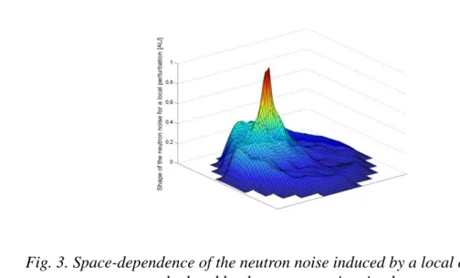
of the channels. Such instabilities are usually referred to as pure DWO or local oscillations. Due to this imposed boundary condition, the two-phase pressure drop in the perturbed fuel channel will create a feedback pressure perturbation of the opposite sign in the single-phase region, either reinforcing or damping the initial perturbation (see Yadigaroglu and Bergles, 1972) This pressure drop oscillation can also be translated into a perturbation of the coolant density (explaining the name of DWO for this kind of perturbation). The typical frequency at which such oscillations are encountered is around 0.5 Hz, which is related to the transit time of perturbations from the inlet to the outlet of the fuel assemblies. This type of oscillation typically occurs when a fuel assembly is unseated, i.e. does not sit properly on the lower fuel tie plate of the core. Since each fuel assembly in a BWR is contained in a fuel box, the fuel channels are independent from each other. Therefore, in case of an unseated fuel assembly, some of the coolant bypasses the fuel channel. This reduces the single-phase pressure drop at the inlet of the channel, and destabilizes it. Radially, this perturbation is equivalent to a local noise source, or a so-called absorber of variable strength-type of noise source and can be modelled by the neutron noise simulator developed at the Department of Nuclear Engineering, Chalmers (Demazière, 2004). An example of the results of such a modelling is presented in Fig. 3. The induced neutron noise has thus its largest amplitude at the position of the noise source, and has a fast spatial decay away from it. Instabilities due to the void-reactivity feedback may also occur in a BWR. The mechanism driving this kind of oscillation is mainly the time-delay between a given power perturbation and the corresponding reactivity response due to the void/pressure coefficient. In some cases, the initial perturbation can be reinforced by the void/pressure feedback if the phase of this delayed response coincides with the phase of the power perturbation. It has to be emphasized that these instabilities also involve density waves through the core, but such waves alone are not responsible for the oscillations. Two types of instabilities involving such a coupling between the neutron kinetics and the thermal-hydraulics are usually encountered: in-phase (or global) oscillations, and out-of-phase (or regional) oscillations. In order to better understand the spatial dependence of such oscillations, the neutron flux can be expanded on the eigenfunctions of the system as:

Fig. 3. Space-dependence of the neutron noise induced by a local oscillation as calculated by the neutron noise simulator

(20)

( , ) _n( ) ( )_n

n

t a t

r r (6)

where _n( )r represents the eigenfunction of the system of order n. For the sake of simplicity, assuming one group of delayed neutrons, a homogeneous reactor, and one-group diffusion theory, one could demonstrate that (the interested reader is referred to Lamarsh (2002) for the derivation of the following equations):

( ) exp( )

n n n

a t A t (7)

where A_n is a constant, and _n fulfils the following ―in-hour‖ equation:

1 1 n n n n t t t (8) with 2 1 ( ) n a n t v B D (9) and 2 n

B is the geometrical buckling corresponding to the eigenmode n. One can easily show that

1 0 (10)

2 1

... 0 (11)

and ₀ is the only of the _n that can be positive.

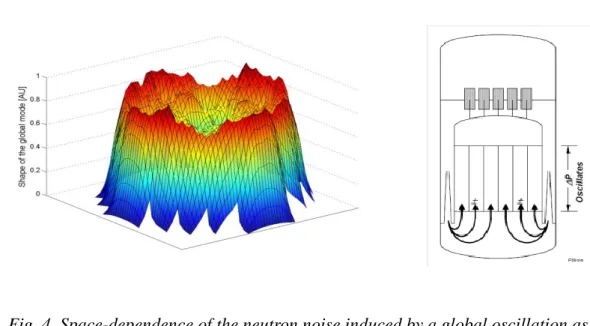
For the global (in-phase) oscillation, the flux is oscillating over the whole core at a typical frequency of 0.5 Hz, and only the first neutronic mode (fundamental mode), i.e.

Fig. 4. Space-dependence of the neutron noise induced by a global oscillation as calculated by the neutron noise simulator (on the left hand-side) and conceptual illustration of the in-phase behavior of the flow and power oscillations (on the right

(21)

0

n , is excited. This is explained by the fact that the reactivity ₀ of the fundamental mode is the only one that can be larger than zero and correspondingly w₀ can be positive. The space-dependence of the flux is thus following the first neutronic mode. Due to the global character of the perturbation, the flow oscillations induced by the void/pressure oscillations are damped by the friction in the recirculation loop, and the recirculation loop dynamics has a stabilizing effect. The neutron noise induced by such an instability can be modelled by the neutron noise simulator, since the different eigenfunctions can be estimated by this tool. An example of the results of such a modelling is presented in Fig. 4.

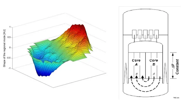
For the out-of-phase (regional) oscillation, the second and third neutronic mode (first and second azimuthal modes), i.e. n = 1 and 2, are excited. Such modes are subcritical and should decay in time in an exponential manner. Nevertheless, the excitation of such modes leads to positive flow rate perturbations in one half of the core counterbalanced by negative flow rate perturbations in the other half of the core at any time in such a way that the boundary conditions imposed by the recirculation loop are always fulfilled. As a consequence, such oscillations are self-sustained by the thermal-hydraulics. The neutron noise induced by such an instability can also be modelled by the neutron noise simulator. An example of the results of such a modelling is presented in Fig. 5. One characteristics of the regional oscillation is that several higher modes can be excited, compared to only one for the in-phase oscillation. Typically, the second and third modes, i.e. first and second azimuthal modes respectively, are excited. Even if these modes are subcritical, the thermal-hydraulics might self-sustain the oscillations. The oscillation frequency of these two modes, although typically close to 0.5 Hz, might be slightly different from each other. Thus, the resulting oscillation, which is the sum of these two modes, might exhibit a rotating neutral line, with the neutral line being defined as the

Fig. 5. Space dependence of the neutron noise induced by a regional oscillation as calculated by the neutron noise simulator (on the left hand-side) and conceptual illustration of the out-of-phase behavior of the flow and power oscillations (on the right

(22)

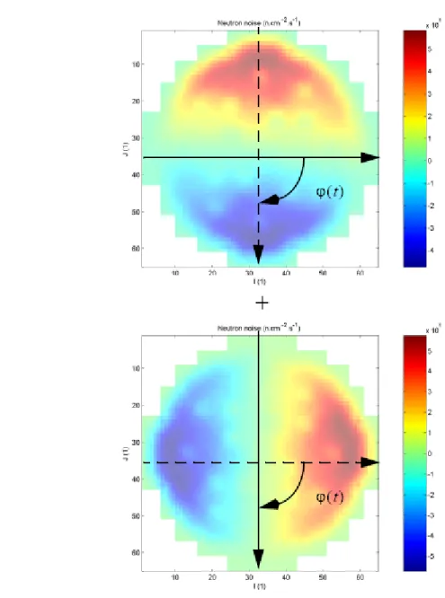
line separating the positive and the negative lobes of the oscillation. An equivalent formulation is to say that there exists a phase shift between the first and second azimuthal modes, and that this phase shift is time-dependent, as illustrated in Fig. 6. Very often, a fourth mode, i.e. the first axial mode, can also be excited. The regional or out-of-phase oscillation is thus a complicated oscillation due to its spatial intermittence, i.e. the neutral line might be stable or it might rotate.

1.6 Combined types of oscillations

When instability events occur at nuclear power plants, several types of oscillations are usually excited simultaneously, even if typically only one is predominant. This complicates significantly the estimation of the DR, since as explained earlier, the DR is

Fig. 6. Definition of the time-dependent phase shift between the first and second azimuthal modes

(23)

based on the assumption that only one type of oscillation exists. Furthermore, it is customary to estimate the DR from the LPRMs, i.e. a value of the DR is estimated for each LPRM. One direct consequence of using local measurements for estimating a global parameter such as the DR is that the estimations might exhibit a space-dependence.

If only one type of oscillation is excited, then the DR is the same throughout the core. If several types are excited, the DR might become space-dependent. This can be demonstrated by assuming that the oscillations of the neutron flux can be written as a sum of the contributions of two oscillating modes, due to two different noise sources i (i 1,2), each of them being factorized into a temporal part only and spatial part only

( ( ))_i r . In such a case, the DR, defined as the ratio of the first and the second maxima of the ACF, is given by (Pázsit, 1995):

2 1 ( ) _i( ) _i i DRr c r DR (12) with 1 ( ) , ( ) In( ) 1 ( ) In( ) i j i i j c i j DR C DR r r r (13)

This expression was obtained assuming that each oscillation mode i has the same resonance frequency but different stability properties, i.e. DRs. Furthermore, it was supposed that the CPSD between the two noise sources is negligible, and that the DR of any of the two noise sources was larger than 0.4. _i( )r represents the radial space-dependence of the neutron noise induced by the noise source i. This spatial space-dependence can be estimated by the neutron noise simulator for all types of BWR instabilities

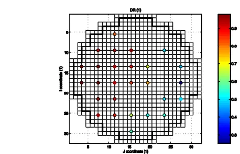
Fig. 7. Simulated radial space-dependence of the Decay Ratio in case of a local noise source and a global noise source (the white square represents the location of the local

(24)

(global, regional, or local oscillations). The coefficient C represents the ratio between the strength of the noise sources and is a normalization coefficient. The DR exhibits a strong radial space-dependence only when there are at least two types or sources of instabilities in the core with different stability properties, and at least one of those correspond to a local oscillation.

The case of a local oscillation coexisting with a global oscillation is shown in Fig. 7. The reason of the sharp boundary between the two stability regions when at least one local noise source exists is the fast spatial decay of the amplitude of the local oscillations. Such a pattern for the spatial dependence of the DR was actually noticed at the Forsmark-1 BWR, as can be seen in Fig. 8, during the channel instability event already mentioned in 2.5c(i) (the interested reader is referred to Oguma, 1997). Eqs (12) and (13) allow explaining the space-dependence of the DR in the Forsmark case, since a local oscillation could be triggered by an unseated fuel assembly.

In order to correctly estimate the stability properties of a BWR, it is thus essential to separate the different types of oscillations from each other. Thereafter, the stability of each mode can be characterized by a DR per oscillation mode. Different techniques have been elaborated for monitoring the stability of BWRs and for separating the different modes of oscillations.

Whereas the global oscillations can be properly detected by the Average-Power Range Monitors (APRMs), the LPRMs are necessary to characterize the regional oscillations. The monitoring techniques that are capable of detecting different types of oscillations can basically be classified into three categories, which are briefly explained in the following in increasing order of sophistication.

Fig. 8. Radial space-dependence of the DR determined at the Forsmark-1 BWR during the 1996/1997 channel instability (derived from Oguma, 1997)

(25)

The first class of techniques aims at monitoring the phase difference between pairs of symmetrically-located LPRM detectors. A phase shift approaching 180 deg indicates out-of-phase oscillations, whereas a negligible phase shift indicates in-phase oscillations. The drawback of these techniques is the difficulty in monitoring combined modes of oscillations.

The second category of techniques is based on the determination of the part of the LPRM signals related to the in-phase oscillations, using for instance the property of orthogonality between the fluctuations of the shape function of the neutron noise and the static flux. This leads to

0 2 0 0 ₀ ( , ) ( ) ( ) ( , ) ( ) _{( )} pk t d P t t P _d r r r r r _{r r} (14)

Subtracting this in-phase component to each of the LPRM signals also allows detecting possible out-of-phase oscillations.

The last class of techniques is based on modal decomposition of the neutron noise. In this procedure, the neutron flux is expanded in the eigenfunctions of the system as:

( ) _n( ) _n n t a t (15) with † † , ( ) ( ) , n n n n F t a t F (16)

Fig. 9. Time-dependence of the expansion coefficients for the three first modes applied to the LPRM signals during a stability test at the Ringhals-1 BWR

(26)

In these equations, the vector ( )t represents the space- and time-dependent neutron flux (where each element of the vector represents the value of the time-dependent flux at a spatial point in the system), _n represents the space-dependent eigenfunction of mode n, †

n is its adjoint, and F is the fission operator. This decomposition can be

performed either with the prior determination of the different modes of the static neutron flux or without it. An example of such a modal decomposition applied to a stability test performed at the Swedish Ringhals-1 BWR is represented in Fig. 9. As can be seen in this figure, both the global and the regional oscillation patterns are excited in the analysed stability test. It is interesting to notice that both the global and regional oscillations are clearly intermittent, and that they sometimes exhibit growing amplitudes over a couple of periods. Furthermore, it can also be seen that the phase shift between the first and second azimuthal modes is varying with time. As a consequence, the regional oscillation, which is a combination of these two azimuthal modes, will be characterized by a rotating neutral (nodal) line.

(27)

2 An investigation of the significance of the

properties of the noise source for BWR instability

2.1 Introduction

In conceptual interpretation of the stability properties of boiling water reactors often a simplified model is used which assumes that the power or flux oscillations in the core can be described as the response of a damped linear oscillator, driven by a white noise driving force. It is obvious that such a model describes the behaviour of the system only in the linear regime, whereas fully developed instabilities are non-linear in character. However, such a model still proves useful in understanding the path to instability, especially the interplay of several different oscillation modes (global, regional, local) (Pázsit, 1995; Demazière and Pázsit, 2005). In such models of the BWR dynamics, it is always assumed that the driving force has a white noise spectrum, i.e. it is constant in frequency. However, the situation becomes different if the APSD of the driving force has a frequency dependence (``coloured noise''). In principle there are two situations when estimating system properties with the assumption of white driving source can lead to erroneous estimation of the decay ratio. One is if the driving force has resonances of its own, which can be interpreted as system resonances. Such resonances are known to occur in form of standing waves in the primary circuit of PWRs, and their presence can complicate the understanding of the properties of the flow induced vibrations of PWR internal structures. A slight resonance of the driving force close to the oscillation frequency of the system resonance can shift into the system frequency due to change in the parameters determining the force properties. This would then occur as a change in the system properties (stability). Another possibility is if the driving force has a sink (dip) at the system resonance that leads to a resulting system response which, when interpreted as only due to system properties as induced with a white driving force, would indicate a stable system. This should be a potentially dangerous situation, since the presence of an instability would not be observed until there is a shift in the sink frequency of the driving force, leading then to a much more unstable system behaviour. The driving force in our model is represented by the reactivity perturbation, which are generated by the propagating density fluctuations of the two-phase flow. The thought on the possible role of the changed properties of a none-white driving force is supported by the fact that the instability occurs at a certain point of flow and power values on the power-flow map, and disappears when the operational point is moved on the map. This may be primarily due to the dependence of the system properties on the flow conditions. However, according to the above reasoning, the properties, and in particular the sink structure of the driving force, are also changing with the changes in flow velocity. Then, the change in the stability properties of the system response may be influenced also by the properties of the driving force.

Assuming that the driving force has a frequency spectrum equal to that of the reactivity effect of propagating two-phase flow the system response to such a perturbation, and in particular the ACF (auto-correlation function) of the response can be calculated analytically. This will be described in the following sections. The response is then compared to that obtained from the same system with a white driving force, and the

(28)

possible error in the estimation of the system response by assuming a white driving force is calculated.

2.2 Calculations for a white noise driving force

The solution of this classic case has known been long, and one re-derivation is found e.g. in (Pázsit I. (1995)). Since a similar methodology will be used for the case of a coloured noise driving force, we briefly repeat here the main steps of the calculation. The damped oscillator is described by the second order equation:

2

0 0

( )t 2 ( )t ( )t f t( ). (17) where f t( ) stands for the driving force. With a temporal Fourier transform of (17) and using the Wiener-Khinchin theorem, one obtains APSD of ( , )r t as:

2 2 2 2 2 2 2 0 0 ( ) | ( ) | , ( ) 4 f APSD APSD H C (18)

where C stands for the constant APSD of the driving force and H( ) is the system transfer function. The autocorrelation function is obtained by an inverse Fourier transform of APSD ( ), for which the poles of |H( ) |2 need to be determined. If one only considers cases when the decay ratio e 2 0.5, then neglecting terms of

2

( )

O besides unity, the APSD poles can be presented as:

1,2,3,4 0(1 i ).

The ACF can now easily be calculated by the theorem of residues. The details are not given here since the calculation is straightforward. For the numerical values of that are usually encountered, the result is given as

0 | | 0 3 0 ( ) cos( ). 4 C e ACF (19)

The form Eq.(19) will be used to determine the decay ratio and resonance frequency from the noise induced by a coloured driving force in the forthcoming analysis.

2.3 The reactivity effect of propagating perturbations: a non-white

driving force.

Now we consider the case of a driving force with non-constant spectral content. The spectral form of the driving force will be taken as the reactivity effect induced by a propagating perturbation with a white noise at the inlet. This type of driving force was studied extensively in the early 70'es as a model for the reactivity perturbations induced by the inlet temperature fluctuations of the coolant in a PWR (Kosály. and Williams, 1971; Kosály and Meskó, 1972; Pázsit, 2002). The model used in the above publications assumes that the perturbations entering the inlet propagate axially along the whole height of the core unchanged which is not really valid for two-phase flow. However, some basic features of the perturbation, such as the presence of peaks and sinks (will be seen below), are expected also from the boiling noise. At any rate, this appears to be a suitable model for a non-white driving force with some relevance to realistic cases. As is described in the above publications, the propagating perturbation is defined by the relationship:

(29)

( , ) 0, .

a a

z

z t t

v (20)

From here it follows that the frequency dependence of _a( , )z t is given as:

( , ) (0, ) .

i z v

a z a e (21)

Then, the reactivity in first order perturbation theory is defined as:

2 0 1 ( ) ( ) ( , ) , H a f t z z t dz (22)

which in the frequency domain becomes:

2 0 (0, ) ( ) ( ) . H i z a v f z e dz (23)

From here, with an application of the Wiener-Khinchin theorem and using the normalized flux ( )z 2 sin z,

H H , one obtains the following expression for

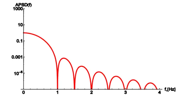
reactivity APSD: 2 4 6 2 2 4 2 2 2 32 (1 cos ) ( ) . ( _f) _T k v T APSD H (24)

where T H v and / T 2 /T 2 v H/ . Here T stands for the transit time of the

perturbation in the core and _T is the corresponding angular frequency. As is easy to show, the function above has no poles at 0 and _T . On the other hand,

( )

APSD has a sink structure, i.e. has zeros at:

; 2,3,

n n T n (25)

An illustration of this APSD is shown in Fig. 10 as a function of the frequency.

The transit time was selected as T 2 sec, which is a typical value of the coolant in BWRs, leading to the characteristic frequency 0.5

2 T T

f Hz. Hence the sink frequencies f_n are equal to f_n n f_T, n 2,3 . According to experience, the core resonance frequency f₀ is also equal to the inverse of the transit time of the coolant in the core, so that f_T f₀, or _T ₀. However, in the investigation of the properties of the induced noise, we will decouple these two variables and investigate cases when they are not equal to each other.

Interestingly, the autocorrelation function of this reactivity APSD of the propagating perturbations was never written down. One way to do that is the Fourier-inversion of (24) which is not trivial, and will be implemented in the next Section. Alternative way is based on the observation that the white noise character of _a(0, )t can be expressed by:

(30)

Fig. 10. APSD of the reactivity fluctuations due to propagating perturbations T 2s, 0.5 T f Hz. 2 (0, ) (0, ) ( ). a t a t k t t (26)

Then, writing t t and utilizing the traditional definition of ACF as a time convolution, one has:

2 2 2 2 0 ( ) ( | | ) if | | . ( ) ( ) 0 if | | H f vk d z z z v T ACF T (27)

Physically, this means that since the perturbation enters at the inlet with a zero correlation time (white noise), spatial correlations of the noise can only be found between points that belong to the same entry, and such can only be found for time differences less or equal to the time T of the perturbation passing the core, which is therefore the maximum correlation time of the driving force.

Performing the integral leads to the final result:

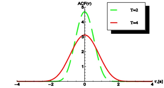
2 2 2 3 ( ) ( | | )(2 cos ) sin | | ( | |). 2( _f) T 2 T vk H ACF H v T H (28)

Some examples of this autocorrelation function are shown in Fig. 11.

2.4 Calculations for the non-white driving force.

We will now assume that the APSD of the driving force f t( )of Eq. (17) has the same functional form, i.e. the same frequency dependence as that of the reactivity

(31)

perturbations, but we omit the constant factors such that the notations become simpler. Then one has:

2 2 2 2 1 cos ( ) . ( ) f T T APSD (29)

With this APSD of the driving force one obtains for APSD the expression:

2 2 2 2 2 2 2 2 2 2 2 0 0 (1 cos( )) ( ) ( ) | ( ) | , ( ) 4 ( ) f T T APSD APSD H (30)

where APSD_f is given by (29), and the transfer function H( ) | is the same as given before.

Determination of the ACF from (30) with inverse Fourier transform goes along the same lines as before. One needs to determine the poles of APSD . These come partly from the poles of |H( ) |2which are the same as before and partly from APSD_f , which are quite specific and create some peculiarities in ACF function.

Namely, it can be shown that for the asymptotic part of the ACF, defined as the part of the curve for T , the ACF will show exactly the same decaying oscillation character,

and hence also lead to the same decay ratio, as with a white noise driving force. Consequently, it will also show the true decay ratio. That happens since APSD_f doesn’t give any contributions into poles for T but does for T . In a general setting this

result means that the ACF of the noise oscillations induced by a coloured driving force will deviate from those induced by a white driving force over the correlation time of the driving force. We will call this the transient part of the ACF. If this correlation time is finite, as in the present case, then the transient part will be finite, followed by an asymptotic part of the ACF of the induced neutron noise which will not differ from that induced by a white noise driving force.

Fig. 11. The ACF of the reactivity effect of propagating perturbations for two different transit times.

(32)

The calculations needed for the Fourier inversion of (30) were performed by using Mathematica. After extensive algebra, for the case of small as in the case of the white driving force, one obtains:

0 0 0 | | 0 | | 0 | | 0 4 5 4 0 ( ) cos | | [| |] 0.5 cos | | [| |] 0.5 cos | | [| |] 4 ( | |)( cos ) sin | | [ | |], 128 T T T T ACF e A e A T T e A T T T T F Y T (31)

Where A B F Y₁, ₁, , are complicated functions of system parameters , ₀,T.

The correctness of the above solution was checked both by Fourier-transforming it back to the frequency domain by Mathematica, and by calculating the inverse Fourier transform of (30) with a numerical FFT routine and comparing it with (31).

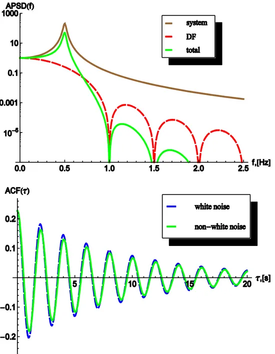
2.5 Analysis of the results

We shall now analyse the results both qualitatively and quantitatively for case when

0 T 0.5

f f Hz, corresponding to a transit time of T 2sec. The corresponding APSD of the driving force was shown in Fig. 10. From the stability point of view this frequency spectra can demonstrate two interesting cases: one when we have a strongly damped system (fast decaying ACF, low decay ratio) corresponds to a wide peak in the system transfer APSD, and an unstable system (slowly decaying ACF) corresponds to a narrow resonance. At the same time, the corresponding ―measured‖ ACF will be different from that of the transfer function alone. We shall call this the virtual APSD or ACF, as opposed to the ``true'' one which belongs to the transfer function. Namely, if the driving force has a narrow resonance around the peak frequency of the system resonance, then the "virtual" APSD will be narrower (higher decay ratio), than that of the true system, meaning better system stability than the one deduced from the measurements. From the operating point of view, on the other hand, this situation is disadvantageous, since the load on the system due to the large amplitude power oscillations is just as large as in the case of high true DR.

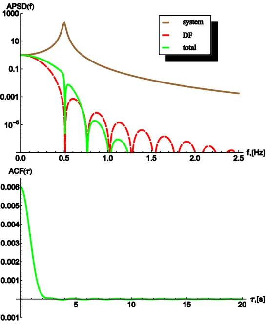
The other possibility of a significant difference between the virtual and the true stability is when the APSD of the driving force has a deep local minimum at the peak frequency of the system resonance. In that case the peak of the induced noise APSD will be broader than that of the system resonance, hence the stability deduced from the measurements is larger than the true one (the virtual DR is smaller than the true one). This means that the driving force in this case suppresses the power oscillations, which is advantageous for the operation. The potential danger of the situation is that a possibly highly unstable state of the system goes unnoticed. However, none of the above cases occurs in our model ( ₀ _T,f₀ f_T) which can be seen in Fig. 12 with a true DR of the system being equal to 0.8. As seen from the Figure, since the driving force has the first sink at 2f_T, the frequency dependence of the driving force is smooth over the resonance frequency f₀, without any peaks. Consequently, the width of the resonance of the measured signal (the ``virtual'' resonance) is very similar to that of the system

(33)

resonance. In that case, having DR=0.8, the resonances for both the system and the arising noise are relatively narrow.

One can study various further cases by keeping f₀constant and changing f_T.Increasing

T

f will not yield any qualitatively new result simply giving smoother behaviour of the noise source APSD over the system resonance at f₀. A more interesting case is when f_T

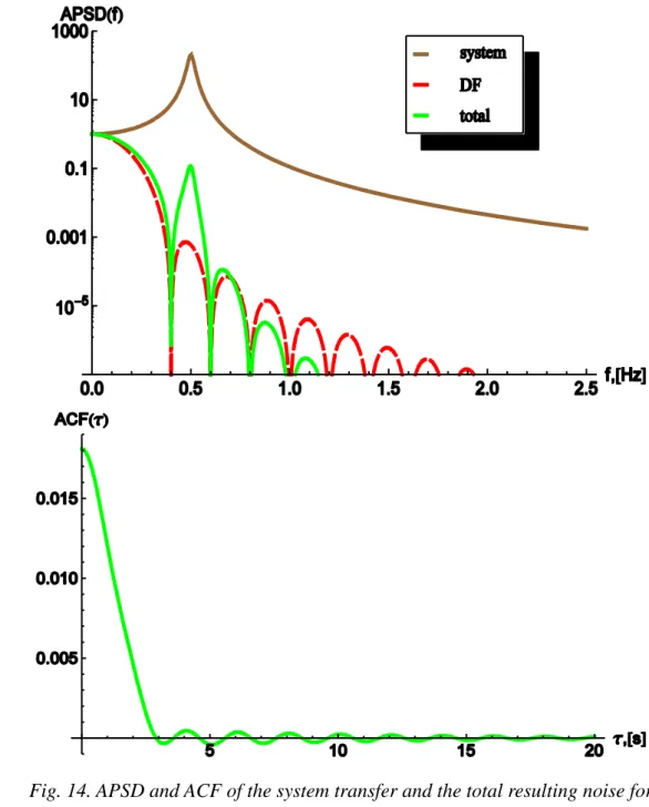
is decreased, such that the first sink of the driving force starts to approach the resonance of the transfer function. At f_T f₀/ 2 the first sink of the APSD of the driving force

Fig. 12. APSD and ACF of the system transfer and the total resulting noise for

0 0.5

T