00:28 Research and Development Program in Reactor Diagnostics and Monitoring with Neutron Noise Methods

SKI Report 00:28

Research and Development Program in

Reactor Diagnostics and Monitoring with

Neutron Noise Methods

Stage 6. Final Report

ISSN 1104-1374

I. Pázsit

C. Demazière

S. Avdic

B. Dahl

July 2000

SKI Report 00:28

Research and Development Program in

Reactor Diagnostics and Monitoring with

Neutron Noise Methods

Stage 6. Final Report

I. Pázsit

C. Demazière

S. Avdic

B. Dahl

Chalmers University of Technology

Department of Reactor Physics

SE-412 96 Göteborg

Sweden

July 2000

This report concerns a study which has been conducted for the Swedish Nuclear Power Inspectorate (SKI). The conclusions and viewpoints presented in the report are those of the authors and do not necessarily

Research and Development Program in Reactor Diagnostics

and Monitoring with Neutron Noise Methods: Stage 6

Summary

This report gives an account of the work performed by the Department of Reactor Physics, Chalmers University of Technology, in the frame of a research contract with the Swedish Nuclear Power Inspectorate (SKI), contract No. 14.5-991060-99180. The present report is based on work performed by Imre Pázsit (project leader), Christophe Demazière, Senada Avdic and Berit Dahl.

This report constitutes Stage 6 of a long-term research and development program concerning the development of diagnostics and monitoring methods of nuclear reactors. The long-term goals are elaborated in more detail in e.g. the Final Reports of Stage 1 and 2 (SKI Rapport 95:14 and 96:50, Refs. [1] and [2]). Results up to Stage 5 were reported in [1] - [5]. A proposal for the continuation of this program in Stage 7 is also given at the end of the report.

The program executed in Stage 6 consists of three parts and the work performed in each part is summarized below.

Investigation of the possibilities of using the neutron current for diagnostics

In Stage 5 experimental and numerical investigations were made of the applicability of using the gradient of the static flux to locate a neutron source in a water tank. The measurements were made with a recently developed very small optical fibre detector, and the supporting calculations done with the Monte Carlo code MCNP. In the present Stage, the work was extended to the investigation of the true neutron current. Based on the same thin fibre detector that was used in earlier work, a detector capable of measuring the neutron current was constructed. This was achieved by covering one side (half of the perimeter) of the detector with a cadmium cladding. With this detector, laboratory measurements were carried out the same way as with the gradient detector in the previous stage. A neutron source located in a water tank was used and the flux and the current measured in points with varying distance from the source. The direction of the neutron current vector indicates the direction (polar angle) of the source from the measurement point, and the ratio of the absolute value of the current to the flux can be used to estimate the distance to the source.

For the latter, values of the same ratio as a function of the source-detector distance must be available from theory or calculations. We have used earlier MCNP calculations of the gradient/flux ratio for this purpose. The results show that it is possible to measure the true neutron current with the detector construction and, by comparing them to MCNP calculations, to determine the distance to the source and thereby also determine the position of the source.

Numerical calculation of the noise and the transfer function in inhomogeneous reactors In the previous stage, we have developed a numerical finite-difference code which can be used to calculate the dynamic adjoint (i.e. the transfer function) in a heterogeneous 1-D reactor system and in two-group diffusion theory. The purpose in this Stage was to extend the calculations to 2-D and 3-D cases. This was achieved by a finite difference scheme,

similarly to the one used in the previous stage. Actually, a relatively large and involved computational tool was elaborated, containing several modules. In the first module the static, space-dependent group constants are generated, to be used as input by the finite difference dynamic code. These are calculated through CASMO/SIMULATE for a realistic heterogeneous core. The dynamic code then calculates the noise for a number of hypothetical perturbations. The perturbations can be given either as direct changes in the cross-sections, or changes in the temperature of various components (coolant, fuel etc.). In the latter case the temperature fluctuations are converted into cross-section fluctuations by another module. Finally the noise is calculated in two or three dimensions by using the static group constants, the time derivatives, the delayed neutron data and the perturbations data. By a suitable choice of the perturbation, the Green’s function can also be calculated, from which the noise induced by other perturbations can be calculated by integration. The model was verified through comparison to analytical calculations.

Preliminary investigations of the application of noise analysis for the determination of the moderator temperature coefficient (MTC)

It has been proposed a long time ago that the cross-correlation or coherence between the neutron noise, measured locally in the core, and the core-exit thermocouples can be used to determine the MTC. Such a method would have large advantages over the traditional ones because e.g. it would not interfere with the reactor operation. Earlier investigations showed nevertheless that the MTC value, obtained from such investigations, gave a quantitative value for the MTC that was 2 to 5 times lower than the true one.

One very likely reason for this deviation lies in the fact that in the evaluation of the noise measurement, it is assumed that the temperature fluctuations, driving the neutron noise, are homogeneously distributed in the core, and that the response of the reactor is point-kinetic. In reality none of these two assumptions are fulfilled, because the temperature fluctuations are space dependent. Hence the reactivity effect of the driving source will be smaller than expected, and the induced neutron noise will also be space-dependent (i.e. will deviate from point-kinetics).

In this Stage investigations were made for the case when the inlet temperature fluctuations are not spatially homogeneous, rather are random in space with a finite correlation length. A simple analytical model was set up to describe the spatially randomly distributed noise source. Then, first the space-dependent neutron noise was calculated and its deviation from point-kinetics was investigated. It was found that if the correlation length of the noise source is much shorter than the core size, appreciable deviations from the point kinetic behaviour occur. These alone however cannot explain the observed experimental error in the MTC measurements. Second, the fact that the reactivity effect of randomly distributed sources is smaller than that of the homogeneous perturbations was also accounted for. This was made first by calculating the reactivity effect alone, and then by calculating the space-dependent neutron fluctuations and the MTC in the model and comparing it with the traditional evaluation formula, to obtain the MTC. From this comparison the bias (error) of the traditional formula, due to the deviation of both the reactivity effect and the induced neutron noise from the expected homogeneous and point-kinetics, respectively, could be assessed. It was found that for a correlation length of the noise source that is comparable with the dimensions of a fuel assembly, the bias of the traditional evaluation formula is in the same range as observed in measurements.

Forskningsprogram angående härddiagnostik

och härdövervakning med neutronbrusmetoder: Etapp 6

Sammanfattning

Denna rapport ger en redovisning av det utförda arbetet inom ramen för ett forskningskontrakt mellan Avdelningen för Reaktorfysik, Chalmers tekniska högskola och Statens Kärnkraftinspektion (SKI), kontrakt Nr. 14.5-991060-99180. Rapporten är baserad på arbete utfört av Imre Pázsit (projektledare), Christophe Demazière, Senada Avdic och Berit Dahl.

Rapporten motsvarar Etapp 6 av ett långsiktigt forsknings- och utvecklingsprogram angående utveckling av diagnostik och övervakningsmetoder för kärnkraftreaktorer. De långsiktiga målen med programmet har utarbetats i slutrapporterna av Etapp 1 och 2 (SKI Rapport 95:14 och 96:50, Ref. [1] och [2]). Uppnådda resultat upp till Etapp 5 har redovisats i referenserna [1] - [5]. Ett förslag till fortsättning av programmet i Etapp 7 redovisas i slutet av rapporten.

Det utförda forskningsarbetet i Etapp 6 består av tre olika delar och arbetet i varje del sammanfattas här nedanför på svenska:

Undersökning av möjligheterna att använda neutronstömmen för härddiagnostik I Etapp 5 har vi genomfört en experimentell och numerisk undersökning av möjligheten att använda den statiska flödesgradienten för att lokalisera en neutronkälla i en vattentank. I dessa mätningar har vi använt en nyligen utvecklad, mycket liten neutrondetektor baserad på en optisk fiber med en neutronkänslig topp. Numerisk simulering av mätningarna gjordes med Monte-Carlo koden MCNP. I föreliggande Etapp har detta arbete utökats till undersökningar av användning av neutronström för samma ändamål. Med utgångspunkt ifrån samma smala fiberdetektor som användes tidigare har vi konstruerat en detektor som kan mäta neutronströmmen. Detta uppnåddes genom att täcka ena sidan (hälften av perimetern) av detektorn med ett kadmiumhölje. Med denna detektor, genomfördes laboratoriemätningar på ett liknande sätt som med gradientdetektorn i föregående Etapp. I en vattentank mättes neutronflödet och neutronströmmen på olika avstånd från en neutronkälla. Riktningen hos strömvektorn indikerar då riktningen (polarvinkeln) till källan från mätpunkten, och kvoten mellan beloppet av strömvektorn och neutronflödet kan användas för att skatta avståndet till källan.

Värdet av denna kvot som funktion av avståndet mellan källan och detektorn, bör vara känd från teori eller beräkningar. Vi har använt tidigare erhållna resultat från MCNP-beräkningar av kvoten mellan gradienten och skalära flödet. Resultaten visar att det är möjligt att mäta den renodlade neutronströmmen med den konstruerade detektorn, samt att, genom användning av beräknade värden, bestämma avståndet till källan. Därigenom kan neutronkällans position bestämmas från mätningar i en punkt.

Numerisk beräkning av bruset och överföringsfunktionen i heterogena reaktorsystem I föregående Etapp har vi utvecklat en numerisk finit-differenskod som kan användas för beräkning av den dynamiska adjungerade funktionen (d.v.s. överföringsfunktionen) i en heterogen 1-D reaktorhärd och i två-gruppsteori. Målet i denna Etapp var att utöka beräkningarna från 2-D till 3-D. Detta åstadkommes, liksom i föregående Etapp, med finita differensmetoder. Ett relativt omfattande och avancerat beräkningsverktyg har utarbetats,

innehållande flera olika moduler. I den första modulen genereras statiska, rumsberoende gruppkonstanter som sedan används som indata till finit-differenskoden som i sin tur beräknar brus och överföringsfunktionen. Dessa gruppkonstanter bestäms via CASMO och SIMULATE för en realistisk härd. Den dynamiska koden beräknar sedan bruset, orsakad av olika hypotetiska perturbationer. Dessa perturbationer kan specificeras antingen direkt i termer av förändringar i tvärsnitt, eller i termer av förändringar i temperatur av olika

komponenter (kylvattnet, bränslet osv). I sistnämnda fallet konverteras

temperaturfluktuationerna till fluktuationer i gruppkonstanter med hjälp av en särskild modul. Slutligen beräknas bruset i två eller tre dimensioner genom användning av statiska gruppkonstanter, tidsderivator, data rörande fördröjda neutroner samt data rörande perturbationen. Med lämpligt val av perturbationen, kan också överföringsfunktionen beräknas, från vilken sedan bruset, orsakad av olika andra perturbationer, också kan beräknas via integration. Koden och den underliggande modellen har verifierats genom jämförelse med analytska beräkningar.

Preliminär undersökning av användning av brusanalys för bestämning av

moderatortemperaturkoefficienten (MTC)

Det har tidigare föreslagits att kors-korrelationen eller koherensen mellan

neutronbruset, mätt lokalt i härden, samt utloppstemperaturen, skulle kunna användas för att bestämma MTCn. En sådan metod skulle visa stora fördelar över den traditionella metoden eftersom den ej skulle störa normal reaktordrift. Undersökningar gjorda hittills har emellertid visat att det kvantitativa värdet av MTC som man erhåller från sådana metoder har varit 2 till 5 ggr lägre än det sanna värdet.

En ganska sannolik anledning till denna avvikelse är det faktum att vid utvärderingen av brusmätningar antages att temperaturfluktuationerna som orsakar neutronbruset är fördelade homogent i härden, och att reaktorsvaret är punktkinetiskt. I praktiken är inget av dessa två antaganden uppfyllda, eftersom temperaturfluktuationerna är rumsberoende. Som en följd av detta, blir reaktivitetsinverkan av bruskällan avsevärt mindre än förväntat, och vidare blir det framkallade neutronbruset också rumsberoende (dvs avviker från den punktkinetiska).

I denna Etapp har vi genomfört en undersökning för det fall när fluktuationerna i inloppstemperatur är ej homogena i rummet, utan är stokastiskt fördelade i rummet och med en ändlig korrelationslängd. En enkel analytisk modell har konstruerats för att beskriva den i rummet slumpmässiga bruskällan. Det rumsberoende neutronbruset beräknades och dess avvikelse från punktkinetik har undersökts. Det visade sig att om korrelationslängden av bruskällan är avsevärt kortare än härddiametern, avviker neutronbruset signifikant från punktkinetik. Endast dessa avvikelser kan emellertid ej förklara det ovannämnda stora felet i den experimentellt bestämda MTCn. Vi undersökte därför kvantitativt effekten av att reaktivitetsinverkan av en bruskälla, slumpmässigt fördelad i rummet, blir mindre än inverkan av en homogen störning. Detta gjordes genom att först beräkna enbart reaktivitetsinverkan hos båda typer av störningar, och därefter genom att beräkna det rumsberoende neutronbruset och även MTCn och jämföra dessa med motsvarande storheter erhållna enligt den traditionella metoden. Från denna jämförelse kunde avvikelsen (felet) härrörande från härledningen av både reaktivitetseffekten och det framkallade bruset med antagande av homogena störningar och punktkinetik, i den traditionella formeln uppskattas. Vi har funnit att om korrelationslängden är jämförbar med dimensionerna av en bränslepatron, vilket verkar överensstämma med mätningarna, är felet av den traditionella utvärderingseffekten i samma storleksordning som det man har erhållit i mätningarna hittills.

Section 1

Measurement of the neutron current and its use for the localisation of

a neutron source

1.1 Introduction

A new method for a direction sensitive measurement of the neutron current or the flux gradient was proposed in [6] to enhance the safety and reliability of nuclear power plants. The use of the information contained in the neutron current or the gradient could improve the diagnostics of various space-dependent anomalies, such as the localisation of vibrating components, channel instabilities, unseated fuel elements, axial position of control rods and so on. The feasibility of detection technique for measurement of the gradient of the neutron flux has been investigated in calculations (Refs. [6], [7]) and in a laboratory experiment by localising a radioactive neutron source in a homogeneous medium ([5], [8]). The flux gradient in two dimensions was obtained from a number of scalar flux measurements performed on the circumference of a circle. The measurements were performed by using a recently developed scintillating fibre detector with a LiF converter for detecting thermal neutrons [9].

In Stage 6 we have performed measurement of components of the neutron current vector. For the measurements a special detector was constructed, using the same thin fibre detector as in previous work. The detector is capable of measuring the partial currents

and in any direction in a two-dimensional plane. From the partial currents, both taken in

two perpendicular directions, the total (net) radial and azimuthal current can be determined. Such measurements were carried out in a static system, composed of a radioactive neutron source located in the centre of a tank filled with water. This system is the same in which the flux gradient was measured, as reported in the previous Stage [5]. The aim of the present measurements is twofold. The first is to investigate the possibility of measuring the neutron current with the newly constructed detector. Current measurements have not been reported in the literature before. The second is to investigate the possibility of localising the source from the measurement of the neutron current and the neutron flux in one single spatial position, and compare the accuracy of the method with the localisation based on the flux gradient. This way a comparative analysis of the angularly sensitive detectors, i.e. the current and the gradient flux detectors, can be made. Finally, any possible deviation between the flux gradient and the neutron current can be explored.

The measurement of the neutron current gave results that are consistent with expectations and earlier results. Based on the results, measurement of the neutron current seems to be a promising alternative for certain core diagnostic tasks.

1.2 Experimental

The measurements were performed using a recently developed very small optical fibre detector [9] whose tip is covered with a mixture of converter material, scintillation material and adhesive paste. With LiF of converter material, detector is sensitive for thermal neutrons. After absorbing a neutron, the resulting ionized reaction products excite the atoms of the scintillating material ZnS into higher atomic levels and they release scintillation light photons by de-excitation. LiF converter and ZnS(Ag) powder are mixed together and pasted J₊ J_{_}

with epoxy glue on the tip of a glass optical fibre of diameter 2 mm. The detector mixture is made thin (~0.3 mm) because of the poor optical properties of ZnS. A layer of opaque paint is also applied on the fibre tip for protection against light and mechanical damage.

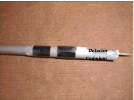
The particular design to measure components of the neutron current is based on shielding the neutron sensitive part of the detector in 180 degrees, in form of a half-cylinder covering the fibre and the tip (Fig. 1). The cadmium absorbs thermal neutrons and thus only

the free side of the detector is exposed to the neutrons. During the measurements, the fibre detector is positioned vertically. As is also seen in the photo, this way the positive and negative partial current components can be measured in a horizontal 2-D plane.

Cadmium has a threshold energy of about 0.5 eV, above which it is transparent for neutrons. Thus, strictly speaking, this detector measures the true partial thermal current only in thermal neutron fields. In our case, especially close to the source, the neutron spectrum is definitively not thermal. Thus the partial thermal current will be contaminated with a component proportional to the epithermal scalar flux. This component is however the same in any partial current measured in one spatial point, and thus it will drop out when taking the difference of two partial currents for obtaining the net current vector component in a particular direction. Thus, although the partial currents will be biased, the net thermal current should be measured correctly with this detector.

The data collection technique is identical with that of the previous work. The light pulses produced in the detector are guided by the optical fibre to a photo-multiplier tube (Hamamatsu R5600U Head-on PMT). The PM-tube is connected via a pre-amplifier (ORTEC 113) to an amplifier (ORTEC 451). After amplification and shaping, the signal is fed into a single-channel analyser (ORTEC 406) and then into a counter/timer (ORTEC 874). A schematic view of the measurement system is shown in Fig. 2.

Fig. 1. Photo Showing the Construction of the Fibre Detector, Measuring the

The measurements were performed in a cylindrical water tank of 92 cm diameter with a radioactive neutron source (3 Ci Am-Be) placed in the centre of the tank. The optical fibre with its neutron sensitive tip was inserted into an aluminium guide tube, which was sealed to protect the fibre from light and direct contact with the water. The tube was put vertically down into the water from a bridge across the water tank. The active part of the neutron detector was positioned on the same horizontal plane as the centre of the source. A thin guiding needle at the tip of the guide tube was put into specific holes drilled in a plastic support plate to place the detector in an exact radial position related to the source. The experimental set-up is shown in Fig. 3.

1.3 Measurement results and analysis

The measurements were performed in several points at different distances from the source. The maximum distance was about 10 cm. The reason for this choice is that the space dependence of both the neutron flux and the current is interesting in a few diffusion lengths vicinity of the source only; at larger distances the flux and the current have a very similar, smooth behaviour that is less interesting. This also means that quantitative localisation of a perturbation is not practical outside of this range, because the distance to the source cannot

HAMAMATSU, R5600U, Head-On PMT. ORTEC 113, Pre-amp. ORTEC 451, Amp. ORTEC 406, SCA LiF and ZnS Optical fibre ORTEC 874, Counter/Timer detector

Fig. 2. A Schematic view of the measurement system

Source

Water

Water tank

Support plate

Aluminium guide tube

Detector position (inside tube)

be determined. However, the direction towards a source or a perturbation can be pointed out from significantly larger distances. This latter question was however not investigated in the present work.

Fig. 4 shows results taken with the ordinary flux detector. It displays the detector count

rate as a function of distance from the source centre and is proportional to the thermal flux. The structure of this dependence was discussed already in the previous Stage. Since the source emits fast neutrons, close to the source the thermal flux is small. Due to the slowing down, both the neutron spectrum and spatial distributions vary with distance from the source. The thermal flux increases with increasing distance from the source and it reaches a maximum at about 3 cm from the source centre. Then it starts to decrease with increasing distance from the source.

This behaviour, verified also by Monte-Carlo calculations, is reconstructed in the present measurements. The error bars shown in Fig. 4 are related only to the statistical uncertainty in the measurements. There is also a possible error due to non-perfect positioning of the aluminium guide tube since it is difficult to adjust the guide tube exactly vertically, i.e. exactly perpendicular to the support plate. This error is difficult to assess and it is not taken into account in the error bars.

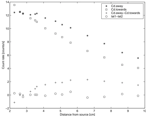
Next, the radial and azimuthal partial currents were measured with the neutron current detector. By turning the cadmium shielded side of the detector towards and away from the source, respectively, the positive and the negative radial partial currents were measured.

Both the partial currents and as well as their difference, i.e. the total (net) radial current

2 3 4 5 6 7 8 9 10 10 15 20 25 30 35

Distance from source [cm]

Count rate [counts/s]

Fig. 4. The Count Rate as a Function of the Distance From the Source

, are shown in Fig. 5. As mentioned earlier, the partial currents may contain a bias, corresponding to the epithermal scalar flux, but the net current should be correct.

In a similar manner, also the azimuthal component of the current was measured. From the cylindrical symmetry of the system, the azimuthal current is zero in this particular case. Nevertheless, it was also determined experimentally, since it gave useful information. The partial currents are not zero, but need to cancel each other. The equality of the partial currents is a good check of the accuracy of the method (quality of the shielding, accuracy of the axial and angular alignment of the detector etc.). Finally, in a real practical case the source position is not known, and symmetry properties cannot be utilized. The values of the net (total) azimuthal current are also shown in Fig. 5.

The results are also shown in quantitative form in Table I. Results obtained for the

radial component of the neutron current J_r, the magnitude of the current (using the radial

and the azimuthal components), the angle of direction towards the source ( ) and the

quantity , as a function of the distance from the source are given in Table I.

The interpretation of the radial dependence of the current is also similar to that of the flux gradient in the previous experiment ([5], [8]). The radial component of the neutron current is equal to the net number of neutrons in outbound radial direction, crossing a unit surface, perpendicular to the radial direction, per unit time. For the first three points located close to the source, this current is negative. The reason is that since the source only emits fast neutrons, thermal neutrons are generated by slowing down of the fast neutrons, which takes them some distance away from the source. Hence, close to the source there is a net influx of J_r = J₊–J_{_} 2 3 4 5 6 7 8 9 10 −2 0 2 4 6 8 10 12 14

Distance from source [cm]

Count rate [counts/s]

Cd.away Cd.towards Cd.away−Cd.towards lat1−lat2

Fig. 5. The Values of the Partial and the Net Currents as Functions of the

Radial Distance From the Source

J

J

∠

thermal neutrons. This behaviour is also in agreement with the Monte-Carlo calculations. Regarding the direction of the measured neutron current, as the Table shows, the neutron current points approximately into the direction towards the source for the points close to the source, and for all others points it is in the opposite (outbound) direction. Thus the measured value of the neutron current vector in any single point can be used to determine the direction where the source is located.

In the Table results are also given for the magnitude of neutron current obtained on the

basis of the two vector components in the x (i.e. ) and the y (i.e. azimuthal) direction.

Statistical uncertainties are obtained from the error propagation formula. The deviation of the

angle from the exact results, i.e. zero or , gives a good indication of the total

measurement error in the experimental determination of the direction. For points at the distance of 2.6 cm and 2.78 cm, the angle of the current direction is approximately equal to

90 because the magnitude of the x-component of the current is close to zero at those

distances. The estimated statistical errors cannot explain the deviation of the calculated

angles of direction from the expected results of zero or . Most probably this is due to

the non-perfect alignment of the guide tube and non-perfect positioning of a Cd layer exactly around half of the detector so the statistical error is only a small fraction of the total measurement error. From results given in the Table, it is seen that it is sufficient to measure only the radial component of the neutron current in order to determine the direction where the source is located. The azimuthal component does not contain this information, but it contributes to the determination of the magnitude of the neutron current vector.

However, to locate the position of a neutron source it is necessary to use the magnitude

of both the current and the flux i.e. the quantity in dependence on the distance from

Table I. Results Distance from source [cm] J_r [cm-1s-1] [cm -1_] [cm-1 s-1] [ ] 2.27 -1.130 0.184 1.159 0.221 167.15 0.19 0.0374 0.0075 2.60 -0.017 0.177 0.170 0.193 95.82 1.14 0.0053 0.0061 2.78 -0.016 0.173 0.293 0.182 -93.24 0.62 0.0093 0.0059 3.22 0.523 0.167 0.524 0.174 2.46 0.33 0.0167 0.0057 3.50 0.935 0.166 0.935 0.172 2.37 0.18 0.0305 0.0059 3.60 1.265 0.165 1.266 0.169 1.34 0.13 0.0420 0.0060 4.10 1.546 0.153 1.550 0.164 -4.16 0.11 0.0540 0.0062 4.71 1.858 0.145 1.869 0.159 6.10 0.09 0.0684 0.0065 5.10 1.873 0.137 1.874 0.142 1.97 0.08 0.0704 0.0060 5.60 2.232 0.128 2.283 0.151 12.07 0.07 0.0889 0.0068 6.60 2.305 0.111 2.338 0.128 -9.74 0.06 0.1085 0.0070 7.60 2.069 0.096 2.089 0.108 -7.84 0.05 0.1118 0.0069 8.66 1.840 0.078 1.845 0.084 4.31 0.05 0.1222 0.0068 9.60 1.489 0.069 1.494 0.074 -4.63 0.05 0.1143 0.0068 J J ⁄Φ J J ∠ ° ± ± ± ± ± ± ± ± ± ± ± ± ± ± ± ± ± ± ± ± ± _± ± ± ± ± ± ± ± ± ± ± ± ± ± ± ± ± ± ± ± ± ± ± ± ± ± ± ± ± ± ± ± ± ± ± r 180° ± ° 180° ± J ⁄Φ

the source. The source position can be determined by using the value of at a single measurement position and a calculated curve of the ratio of the magnitude of neutron current vector and the neutron flux as a function of distance from the source. This was already the case in the previous work, where the static flux gradient was used for localisation. The

function was determined by Monte-Carlo calculation, using MCNP-4B.

Calculating the neutron current vector, corresponding to the present experimental arrangement, represents nevertheless a substantially more complicated task. This is mostly due to the more complicated detector geometry (see Fig. 1.). In addition to the geometry of the detector, the spectral effects need also be carefully modelled since, as mentioned earlier, in the vicinity of the source, the spectrum is far from being thermal, rather it is dominated by fast and epithermal neutrons. Thus close to the source the detector signal contains, in addition to the thermal partial current, also a component of epithermal scalar flux. Finally, a further hinder is represented by the fact that the current is not as easily available from MCNP as the scalar flux. Thus, in view of these considerable complications, calculations of the partial currents were postponed to a later stage of the project.

This postponement was further motivated by the fact that the present measurement results, as will be shortly seen below, did not deviate significantly from the measurements of the flux gradient in the previous Stage. This is not very surprising, for the following reasons. As also mentioned earlier, the contribution from the epithermal scalar flux drops out when calculating the net current (difference of the partial currents). Second, although diffusion theory and Fick’s law may not be fully applicable close to the source, in the gradient measurement the gradient of the true scalar flux is used. The scalar flux and its gradient would be incorrectly predicted by diffusion theory and thus the current would be in error, but here we take the gradient of the true scalar flux, which decreases this error. Besides, since the source emits fast neutrons, any thermal neutrons must have collided several times and thus the thermal flux is not so anisotropic as the fast flux close to the source.

For all these reasons here we only compare the measurements of the thermal current with the measurements and calculation of the thermal gradient from the previous Stage. The results are shown in Fig. 6. which displays measured values of the neutron current, the gradient flux and the results of MCNP calculation of the gradient of neutron flux. The gradient flux values have been obtained by measuring the gradient of the true flux, which is not the same as the gradient of the diffusion theory approximation of the flux. There is a good agreement between experimental results far away from the neutron source (where diffusion theory is applicable) but close to the neutron source the measured values show a slight deviation. This is in accordance with theoretical prediction since the neutron current close to the singularities such as boundaries or source is not proportional to the gradient of the neutron flux. This deviation is nevertheless not large. Hence, the measured values of the neutron current and calculated values of the gradient flux show good agreement.

Fig. 7. shows measured values of the current to flux ratio depending on the distance from the source and the results of MCNP calculation for the ratio of the gradient flux and scalar flux. The results of calculation have been normalized to the measurements. The

experimental values of the quantity and results of calculation obtained with

Monte-Carlo technique agree very well. By using the measured value of the only in a single

measurement position together with a calculated curve of this quantity one can find the source position. The deviation between the estimated and the true distance will be analysed after finishing the MCNP calculations of the neutron current.

J ⁄Φ

∇Φ Φ⁄

J ⁄Φ

0 5 10 15 −1 0 1 2 3 4 5

Distance from the source (cm)

Count rate [counts/s]

the neutron current the flux gradient MCNP calculation of the gradient flux

Fig. 6. Measured and Calculated Values of the Gradient and Current

0 1 2 3 4 5 6 7 8 9 10 −0.1 −0.05 0 0.05 0.1 0.15 0.2

The distance from the source

current/flux

experiment MCNP

CONCLUSION

Laboratory measurements of the neutron flux and vector components of the neutron current in a static model experiment, similar to a model problem proposed in [6] have been performed. The experimental system consists of a radioactive neutron source located in the centre of a water tank. The measurements were performed using a recently developed scintillating fibre detector. The results show that it is sufficient to measure the radial component of neutron current at a single point in order to determine direction where the neutron source is located. The direction and the distance to the source can be determined by using the measured values with corresponding MCNP calculations. At this moment of the investigation (without results of the neutron current calculation) it is obvious that measured values of the neutron current obtained with a special detector and calculated values of the gradient flux are in good agreement. The calculation of the neutron current by MCNP code is ongoing.

Section 2

Numerical calculation of the noise and the transfer function in

inhomogeneous reactors

2.1 Introduction

In the previous stage, a one-dimensional two-group noise simulator based on the diffusion approximation was developed. This simulator was able to calculate the flux noise induced by cross-section fluctuations for heterogeneous systems through the use of a finite difference scheme. In the present Stage, the noise simulator was extended to two- and three-dimensional systems. Another major difference with the previous stage lies with the definition of the noise sources and the calculation of the parameters required by each node.

The model developed is suitable to treat several kinds of fluctuations (coolant temperature fluctuations, fuel temperature fluctuations, flow velocity perturbation, modification of the heat exchange coefficient). They can be defined directly by the user through three-dimensional maps and can be used simultaneously or independently of each other. For purposes of further theoretical investigations, the code also offers the possibility of defining the noise sources in terms of macroscopic cross-sections fluctuations. Furthermore, the code is able to handle any realistic core since the static parameters needed by the simulator are extracted from static modelling through the use of the Studsvik Scandpower SIMULATE-3 code ([10]). Another novelty is the way in which the cross-section fluctuations are calculated. The Studsvik Scandpower CASMO-4 code ([11]) is used to tabulate cross-section fluctuations from fuel and moderator temperature perturbation at operating conditions corresponding to the SIMULATE-3 results. Consequently, a thermal-hydraulic model is also included in the code.

In the following, the noise simulator is described in more detail and the finite difference scheme is explained. Then, the noise simulator is benchmarked against analytical solutions for homogeneous two-dimensional systems. Since the purpose of this stage is to investigate the validity of the neutronic calculations, the thermal-hydraulic module was disabled and the noise source was directly defined in terms of macroscopic cross-section fluctuations.

2.2 Description of the code

Overview

The three-dimensional noise simulator developed below relies on two-group diffusion theory and is able to handle any realistic core. A thermal-hydraulic model is also included in the code, so that the fuel and coolant temperature fluctuations are also taken into account. These calculations are performed in the frequency domain, at a frequency defined by the user. The spatial discretization is carried out by a finite difference scheme: the so-called “box-scheme” is used for the neutron noise discretization, whereas the so-called “point-scheme” is used for the coolant temperature noise discretization ([12]). The static space-dependent group constants are extracted from the Studsvik Scandpower SIMULATE-3 and CASMO-4 codes ([10], [11]). The CASMO-4 code is mostly used to carry out the tabulation of the variation of the two-group constants induced by fuel or moderator

temperature fluctuations. These data are tabulated with respect to static fuel and moderator temperatures, so that these static operating points, calculated by SIMULATE-3 for each node, allow retrieving of these parameters very easily. After converting the temperature noise into cross-section noise through the previous data-functionalization, the simulator calculates the neutron noise and the coolant temperature noise. That is, all the other relevant parameters (fuel temperature noise, velocity fluctuations, modification of the heat exchange coefficient) are directly converted from the external noise sources (defined by the user) and the coolant temperature noise via transfer functions internally calculated within the code. Alternatively, the noise sources can also be defined in terms of macroscopic cross-section fluctuations, as is the case in the benchmark presented in this report.

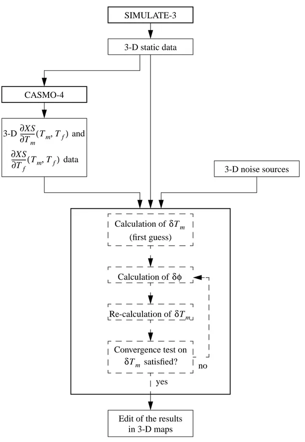
Fig. 8 summarizes the main features of the noise simulator in a block-diagram form. Since the neutronic equations represent a source problem, the neutron noise can be calculated by matrix inversion, as long as the noise sources are known. Due the thermal-hydraulic feedback, this means that an iterative scheme is necessary to calculate the moderator temperature noise and the neutron noise itself.

Calculation of the neutron and temperature noise

In two-group theory, the neutron noise in the diffusion approximation is given by the following set of equations:

(1)

(2)

(3)

Here, all the terms have their usual meaning. The subscript 0 represents the static case, and subscripts 1 and 2 stand for the fast and the thermal groups, respectively. Any time-dependent parameter X is related to its static value according to the generic formula:

(4) If one neglects the second-order terms, subtracts the static equations from Eqs. (1), (2), and (3), and eliminates the precursor density through a temporal Fourier transform, one obtains two equations that can be written in a matrix form as follows:

1 v_{1 0,} ( )r ---∂φ1 t ∂ --- r t( , ) D₁(r t, )∇2φ₁(r t, ) νΣf 1, (r t, ) k_{ef f 0,} --- 1( –β_{ef f 0,} ( )r ) Σ– _{a 1,} (r t, )–Σ_rem(r t, ) φ₁(r t, ) νΣ_{f 2,} (r t, ) k_{ef f 0,} --- 1( –β_{ef f 0,} ( )r )φ₂(r t, ) λ₀( )r C r t( , ) + + + = 1 v_{2 0,} ( )r ---∂φ2 t ∂ --- r t( , ) = D₂(r t, )∇2φ₂(r t, ) Σ– _{a 2,} (r t, )φ₂(r t, ) Σ+ _rem(r t, )φ₁(r t, ) C ∂ t ∂ --- r t( , ) β_{ef f 0,} ( )r νΣf 1, (r t, ) k_{ef f 0,} ---φ₁(r t, ) νΣf 2, (r t, ) k_{ef f 0,} ---φ₂(r t, ) + –λ₀( )r C r t( , ) = X r t( , ) = X₀( ) δr + X r t( , )

SIMULATE-3 3-D static data CASMO-4 3-D and data XS ∂ T_m ∂ --- T( _m,T_f) XS ∂ T_f ∂ --- T( _m,T_f) 3-D noise sources Calculation of (first guess) δT_m Calculation of δφ Re-calculation of δT_m Convergence test on satisfied? δT_m yes no

Edit of the results in 3-D maps

(5)

It is to be noted that due to the temporal Fourier transform, all quantities become complex. Hence in the numerical scheme, complex variables and arithmetic are used.

Due to the data-functionalization performed via CASMO-4, the variation of the two-group constants can be expressed directly from the fuel and moderator temperature fluctuations. The previous equation can then be written as:

(6)

Regarding the thermal-hydraulic model, the fuel and moderator temperatures are described by the following set of equations:

(7)

(8)

(9) All the terms have their usual meaning, and as before, the subscript 0 represents the static case. Expressing all the time-dependent parameters as in Eq. (4), neglecting the second-order terms, removing the static component from Eqs. (7), (8), and (9), and eliminating the time-derivatives by a Fourier transform, the moderator and fuel temperature fluctuations can be expressed in a matrix form as:

(10)

(11)

Spatial discretization

Due to the and operators in Eq. (5) and in Eqs. (10) and (11) respectively, the

spatial discretization introduces a coupling between a node and its neighbours. There are D_∆δφ∇2+D_δφ ( ) δφ1(r,ω) δφ₂(r,ω) D_δD δD1(r,ω) δD₂(r,ω) D_δΣ remδΣrem(r,ω) DδΣa δΣ_{a 1,} (r,ω) δΣ_{a 2,} (r,ω) D_δνΣ f δνΣ_{f 1,} (r,ω) δνΣ_{f 2,} (r,ω) + + + = D_δφ δφ1(r,ω) δφ₂(r,ω) D_δT fδTf(r,ω)+DδTmδTm(r,ω) = m_{f 0,} ( )r c_{f 0,} ( )r ∂Tf t ∂ --- r t( , ) = P r t( , )–h r t( , )S₀( )r [T_f(r t, )–T_m(r t, )] m_{f 0,} ( )r c_{f 0,} ( )r ∂Tm t ∂ --- r t( , ) v_m(r t, )∂Tm z ∂ --- r t( , ) + = h r t( , )S₀( )r [T_f(r t, )–T_m(r t, )] P r t( , ) = V_f( ) κΣr [ _{f 1,} (r t, )φ₁(r t, ) κΣ+ _{f 2,} (r t, )φ₂(r t, )] M_δT m M∂δTm⁄∂z∂z ∂ +    _{ δT} m(r,ω) = Mδvmδvm(r,ω)+Mδhδh r( ,ω)+Mδφδφ(r,ω) δT_f(r,ω) F_δT m F∂δTm⁄∂z∂z ∂ +    _{ δT} m(r,ω)+Fδvmδvm(r,ω)+Fδhδh r( ,ω) = ∇2 z ∂∂

several ways to discretise these operators. A finite difference scheme has been chosen for its simplicity and its efficiency.

All the equations are first integrated on an elementary node. The unknowns are thus expressed by the following generic formulation:

(12)

whereas the elements of the matrices satisfy the relationship:

(13)

This way of volume-averaging is consistent with the definition of the two-group constants given by CASMO and SIMULATE, so that the actual reaction rates are preserved.

If one represents a node I,J,K by the system of axes and numbering as shown in Fig. 9, the spatial discretization of the neutron noise can be carried out according to the “box-scheme” that allows writing ([12]):

(14)

If one takes for instance the x direction, two expressions for can be obtained by

considering the node I,J,K and the node I+1,J,K:

(15) and δX_{I J K, ,} ( )ω _∆ 1 x⋅∆y⋅∆z --- δX r( ,ω)dr I J K, , (

∫

∫

∫

∫

∫

(16) Equating these two expressions allows eliminating the flux noise at the boundary of the two nodes:

(17)

The current noise can thus be determined, so that one obtains:

(18) with (19) (20) δJ_{I J K}y_{, ,} ( )ω δJ_{I J}y_{, –1,K}( )ω δJ_{I J K}z_{, ,} ( )ω δJ_{I J K}z_{, , –1}( )ω δJ_Ix_{–1, ,J K}( )ω δJ_{I J K}x_{, ,} ( )ω x y z where P x( _I, ,y_J z_K) P

Fig. 9. The Principles and Conventions Used in the Discretization Scheme

δJx(x_I +∆x–ε, , ,y_J z_K ω) D_{I J K, ,} δφ(xI+∆x, , ,yJ_∆zK ω) δφ– I J K, , ( )ω x 2⁄ ---– = δφ(x_I +∆x, , ,y_J z_K ω) DI J K, , δφI J K, , ( )ω +DI+1 J K, , δφI+1 J K, , ( )ω D_{I J K, ,} +D_{I+1 J K, ,} ---= δJ_{I J K}x_{, ,} ( ) δω – Jx_{I–1, ,J K}( )ω a_{I J K}x_{, ,} δφ_{I J K, ,} ( )ω +b_{I J K}x_{, ,} δφ_{I+1, ,J K}( )ω +c_{I J K}x_{, ,} δφ_{I–1, ,J K}( )ω = a_{I J K}x_{, ,} 2DI J K, , DI+1 J K, , ∆x D( _{I J K, ,} +D_{I+1 J K, ,} ) --- 2DI J K, , DI 1– , ,J K ∆x D( _{I J K, ,} +D_{I 1– , ,J K}) ---+ = b_{I J K}x_{, ,} 2DI J K, , DI+1 J K, , ∆x D( _{I J K, ,} +D_{I+1 J K, ,} ) ---– =

(21)

For nodes located at the core boundary, the flux at the boundary is known and assumed to be equal to zero, so that the discretised current noise is directly given by

(22) or

(23) depending on which side of the boundary the node is located.

The expression of the coefficient differs slightly from the previous general case

(24)

or

(25)

whereas the coefficient ( coefficient respectively) remains unchanged, and the

coefficient ( coefficient respectively) is equal to zero. Similar expressions can

be obtained for the y and z directions.

Therefore, a discretised matrix formulation can be written for each plane K as follows: (26)

Regarding the thermal-hydraulic equations, the spatial discretization is carried out according to the “point-scheme” that allows writing ([12]):

(27)

Similarly to the neutron noise, one obtains dicretised matrix equations for the fuel and moderator temperature noise:

(28) c_{I J K}x_{, ,} 2DI J K, , DI 1– , ,J K ∆x D( _{I J K, ,} +D_{I 1– , ,J K}) ---– = δJ_{I J K}x_{, ,} ( )ω D_{I+1 J K, ,} δφI+1, ,J K( )ω –0 ∆x 2⁄ ---– = δJ_{I J K}x_{, ,} ( )ω D_{I J K, ,} 0–δφI J K, , ( )ω ∆x 2⁄ ---– = a_{I J K}x_{, ,} a_{I J K}x_{, ,} 2DI J K, , DI+1 J K, , ∆x D( _{I J K, ,} +D_{I+1 J K, ,} ) --- 2DI J K, , ∆x ---+ = a_{I J K}x_{, ,} 2DI J K, , ∆x --- 2DI J K, , DI 1– , ,J K ∆x D( _{I J K, ,} +D_{I 1– , ,J K}) ---+ = b_{I J K}x_{, ,} c_{I J K}x_{, ,} c_{I J K}x_{, ,} b_{I J K}x_{, ,} D_δφK δφK( )ω D_δT f K _δ T_fK( )ω D_δT m K _δ T_mK( )ω D_{u p}K _,δφδφK+1( )ω D_downK _,δφδφK–1( )ω + + + = 1 ∆x⋅∆y⋅∆z --- ∂Tm z ∂ --- r( ,ω)dr I J K, , (

∫

and

(29)

In the two previous equations, external noise sources and have

been added so that the user may define them through 3-D maps if needed.

Combining Eqs. (26), (28), and (29) allows expressing the flux noise in plane K as a function of external noise sources in plane K, the moderator temperature noise of plane K-1, and the flux noise of planes K-1 and K+1:

(30)

Finally, this equation can be rearranged into a matrix equation describing the entire 3-D system:

(31)

In this equation, all the elements of the matrix and the vector are matrixes themselves.

Further, the source is defined as a function of the moderator temperature noise that can be

determined through Eq. (29). Since in this equation the neutron noise must be known in order to determine the moderator temperature noise, an iterative scheme is necessary, as depicted in Fig. 8.

2.3 Comparison to an analytical solution

In this stage, it was decided to benchmark the neutronic calculations of the noise simulator against analytical solutions for homogeneous 2-D systems. Consequently, the thermal-hydraulic module of the calculator was disabled and only one axial plane was used. The noise source was defined directly in terms of macroscopic cross-section fluctuations and is assumed to be located in the middle of the plane. For the present study a perturbation of the fast absorption cross-section was investigated. The calculations were performed at a frequency of 1 Hz.

In the analytical model, the noise source is defined as:

(32)

Since the number of nodes in the numerical model is an even number, an equivalent noise source was defined on the four central nodes and due to the spatial discretization was expressed as: δT_mK( )ω M_δv m K δv_mK( )ω M_δK_hδhK( )ω M_δφK δφK( )ω M_{down δT} m , K δT_mK–1( ) δω T_{m ext}K_, ( )ω + + + + = δTK_{f ext,} ( )ω δT_{m ext}K_, ( )ω F – KδφK–1( ) δφω + K( )ω –GKδφK+1( )ω AKδv_mK( )ω BKδhK( )ω CKδT_{m ext}K_, ( )ω DKδTK_{f ext,} ( )ω EKδT_mK–1( )ω + + + + = ℜδφ ω( ) = S ℜ S S S r( ,ω) S1(r,ω)δ( )r 0 =

(33)

However, there is yet another main difference between the analytical and the numerical model which lies with the difference in the geometry of the respective systems. In the analytical model, the core is cylindrical, with a central source described by (33). This means

that in an geometry, the system is azimuthally symmetric. The case of the numerical

model, on the other hand, is not invariant to azimuthal rotations, since here cubic nodes are put together to represent a cylindrical core, and also the perturbation. Therefore a correction factor to the source strength was calculated to take this effect into account.

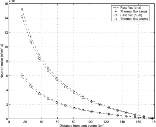
Fig. 10 shows the absolute values of the fast and the thermal flux noise calculated by the noise simulator. Comparison of the fast and thermal neutron noises with the analytical solution are presented in Fig. 11 along a radial line in the core. Since only a volume-averaged neutron noise is calculated by the simulator (see Eq. (12)), the analytical neutron noise was also averaged on each node in order to be compared to the numerical solution. Furthermore, because the calculational time depends mostly on the size of the matrices, i.e. the number of nodes, it was also decided to test the simulator on a coarse mesh. Such a comparison to the analytical solution is presented in Fig. 12. It has to be emphasized that in the case depicted on Fig. 12, the size of a node corresponds to the one used in the SIMULATE-3 calculations. This demonstrates that the spatial resolution of the noise simulator can be selected to be higher than that of a corresponding static SIMULATE calculation. This is an important advantage when the diagnostic task is the localisation of perturbations (malfunctions) in the core ([13]).

S₁(0,ω) 4∆x⋅∆y ---0 r,ϕ ( ) 0 20 40 60 80 100 120 140 160 180 0 2 4 6 8 10 12 14 16x 10 9

Distance from core centre (cm)

Neutron noise (n/cm

2 .s)

Fast flux (ana) Thermal flux (ana) Fast flux (num) Thermal flux (num)

2.4 Conclusions

The benchmarking of the noise simulator against analytical solutions for two-dimensional homogeneous systems shows that the level of accuracy seems to be satisfactory regarding the neutronic calculation and the noise sources investigated so far. If the number of nodes is reduced, the accuracy remains very good. Consequently, using a mesh grid corresponding to the width of a physical fuel assembly should provide reliable

5 10 15 20 25 30 5 10 15 20 25 30 0 0.5 1 1.5 2 2.5 x 1010 Node number Node number

Fast neutron noise (n/cm

2.s) 5 10 15 20 25 30 5 10 15 20 25 30 0 2 4 6 8 10 x 109 Node number Node number

Thermal neutron noise (n/cm

2.s)

Fig. 10. Neutron Noise Calculated by the Noise Simulator in Case of a Fine Spatial

results whereas the parameters required by the simulator could be extracted directly from the SIMULATE-3 calculations without any spatial interpolation.

The work described in this report represents only the first part of the development of the noise simulator, since further benchmarking and improvements are required. First, other types of noise sources need to be investigated and the thermal-hydraulic module has to be tested. Second, only two-dimensional cases have been studied here, whereas the axial coupling of both the neutron noise and the moderator temperature noise represent an important feature of this numerical model, and needs consequently to be benchmarked in more detail. Finally, this model has been developed in the MATLAB environment for the calculational part of the simulator. It is intended to improve the way in which the calculations are performed, i.e. to find more efficient algorithms to solve the problem and to create a source code so that the simulator could be run faster. For practical applications, also parallel computing methods are envisaged.

0 20 40 60 80 100 120 140 160 180 0 2 4 6 8 10 12 14 16x 10 9

Distance from core centre (cm)

Neutron noise (n/cm

2.s)

Fast flux (ana) Thermal flux (ana) Fast flux (num) Thermal flux (num)

Fig. 12. Benchmarking of the Noise Simulator in Case of a Coarse Spatial

Section 3

Preliminary investigations of the application of noise analysis for the

determination of the moderator temperature coefficient

3.1 Introduction

The MTC (Moderator Temperature Coefficient) is an important safety parameter in pressurized water reactors. It has to be measured twice during a fuel cycle in PWRs: at beginning of cycle, hot zero power, to check that the MTC is negative (preventing from the consequences of a power increase), and close to the end of cycle, hot full power, to verify that the MTC remains less negative than some prescribed limit (preventing from the consequences of a cool-down event). Several measurement techniques are in use nowadays (boron dilution method, power change method, depletion method, rod swap method), but none of them are accurate enough since they do not induce a moderator temperature change solely ([14]-[16]).

In the past few years, another measurement technique, relying on the analysis of in-core neutron noise and in-core-exit temperature noise, has been proposed. This technique, which does not require any perturbation of the system, offers the possibility of an on-line and accurate MTC monitoring. There has been an interest in applying this method also at the PWRs in Ringhals.

Nevertheless, all attempts made so far to determine the MTC by noise analysis revealed that such a measurement technique underestimates the MTC by a factor of two to five ([17]-[36]). In order to reduce the discrepancy between the MTC estimate and its actual value, a few improvements in the MTC estimators were introduced ([19], [34], [37]-[41]): to account for the separation distance between the in-core neutron detector and the core-exit thermocouple, to account for the fact that several noise sources may coexist at the same time, and to account for the Doppler effect. These corrections are usually small and cannot explain solely the strong deviation between the MTC calculated by noise analysis and its actual value, so that other hypotheses are also to be investigated. Probably the most important ones among these are the spatially non-homogeneous structure of the temperature noise and the deviation from point-kinetics of the reactor response. Some aspects of these were investigated in the past. In this report we shall give a thorough analysis, including several important aspects that has not been treated at all so far.

The spatial characteristics of both the neutron noise as well as those of the driving force, i.e. the temperature fluctuations, affect the measurement method in more than one way. The traditional method of evaluating the noise measurement assumes not only point-kinetic response of the reactor, but implicitly also the spatial homogeneity of the temperature fluctuations in the radial direction. The significance of first of these two conditions has been generally known, but the second has not been discussed so far.

The significance of the homogeneity (spatially constant character) of the temperature fluctuations is manifold. First, as long as the temperature fluctuations are constant in space, the reactor response will be exactly point kinetic. In that case, all conditions for the applicability of the traditional evaluation formula are fulfilled. If the temperature fluctuations are space dependent, the reactor response will also deviate from point-kinetics.

This fact has been noticed some time ago and was also investigated, although not the same way as in the present work.

However, there are even other, and as it turns out more significant, consequences of the spatial non-homogeneity of the temperature fluctuations as a driving force. The first one is the fact that a spatially incoherent temperature noise will have a much weaker reactivity effect than a spatially homogenous one. The deviation between the true and the assumed reactivity effect yields a bias (error) of the measured MTC, which is space-independent. This fact has not been investigated before. One of the main purposes of the present work was to see the influence of this fact on the determination of the MTC.

The second extra consequence, which was also unexpected to us as well, is that the cross-correlation between temperature fluctuations and neutron noise becomes also smaller than with spatially homogeneous temperature fluctuations. This also introduces a bias to the determination of the MTC. Besides, the cross-correlation between neutron noise and temperature fluctuations, taken in the same spatial position, becomes space-dependent (depends on the spatial position in question).

It is known from experiments that the temperature fluctuations are not spatially homogeneous. Hence the two last effects described above lead to the fact that the measured MTC, which is based on assumptions that do not hold in reality, becomes much smaller than the true one. Thus these phenomena constitute a significant part of the explanation of the discrepancy between the measured and the true MTC.

The significance of the spatial inhomogeneity of the temperature fluctuations was investigated analytically and quantitatively in this Report and will be reported on in this Section. One novelty of the work is that the spatial dependence of the driving force (temperature fluctuations) cannot be given deterministically, only through statistical moments, i.e. through spatial auto- and cross-correlation functions. Thus the theory of neutron noise, induced by spatially random noise sources, had to be elaborated. Concretely, the temperature fluctuations are defined in terms of the Auto-Power Spectrum Density (APSD) and Cross-Power Spectrum Density (CPSD). From these quantities, the statistical behaviour of the flux noise can be calculated. The model developed hereafter allows calculating this flux response in the one-group diffusion theory for a one-dimensional homogeneous bare reactor in two different approximations: either the “exact” solution can be determined through the use of the Green’s function, or the point-kinetic approximation can be applied. Since the MTC can only be defined if the reactor behaves in a point-kinetic way, this model allows also to calculate a biased MTC, i.e. determined from the “exact” flux noise, and to compare it to its point-kinetic definition.

In the following, the theory used to develop this one-dimensional one-group model is explained, and the ways of calculating the MTCs are emphasized. Then, the results of the calculations for a realistic spatially condensed commercial PWR are presented and the effects of heterogeneous random temperature fluctuations are assessed.

3.2 General principles

In the qualitative and quantitative work, a simplified model will be used throughout. Since our purpose is the investigation of the radially inhomogeneous character of the temperature fluctuations, the axial dimension will be disregarded, and a one-dimensional

model is used. The spatial variable is assumed to represent the radial position in the core. In order to calculate the MTC, we will consider inlet temperature fluctuations as noise sources. In principle, in a PWR, these fluctuations travel upwards and are affected by the coolant temperature fluctuations generated inside the core itself. In this model however, the axial dependence of the temperature noise is completely disregarded since the radial dependence of both the temperature and the flux noise is known to give stronger effects. This also means that the inlet and outlet temperatures and their fluctuations are the same, and all generation of temperature fluctuations or their change during the transport of the coolant in the core is neglected. This phenomenon will be however incorporated into later versions of the present model.

Definition of the MTC and its estimation with the noise method

According to the newest American Standard ([42]), the MTC is the reactivity variation due to a change of the inlet temperature of the coolant, divided by the average temperature change:

(34) In general, the reactivity perturbation is related to a change of the macroscopic cross-sections, which in turn are generated by the density changes due to the temperature. We shall assume that reactivity changes are solely due to the change of the absorption cross-sections, since removal cross-sections cannot be treated in the present one-group model. Thus we assume:

(35)

The connection between cross-section fluctuations and the induced reactivity

effect is given by the well-known perturbation formula as:

(36)

Based on the above, the Standard implicitly suggests, due to the expression of the reactivity (Eq. (36)), to calculate the average temperature change by using the square of the static flux as a weighting function:

(37)

In such a case, whatever the spatial structure of the temperature noise might be, Eq. (35) allows calculating the MTC as:

δρ( )t = MT C×δT_mave( )t δT_m(r t, ) = K×δΣ_a(r t, ) δΣ_a(r t, ) δρ( )t δΣ_a(r t, )φ₀2( )r dr

∫

∫

∫

∫

(38)

This MTC is called in the following the “reference” MTC, since it corresponds to the definition given by the Standard, which assumes a point-kinetic behaviour of the reactor.

However, in reality the core-averaged temperature of Eq. (37) cannot be measured. Thus it is assumed instead that the temperature fluctuations are space-independent, i.e.

(39) It is thus assumed that the temperature measured in a given point is the same everywhere in the system. If this holds, one will have

(40) and the expression (38) for the MTC will still be valid. The problem is that in reality (40) does not hold.

In the noise analysis method, the MTC is calculated from the statistical properties of the neutron noise and the temperature noise. Several estimators have been proposed for that purpose ([20], [21], and [23]). Since in our model the flux noise and the temperature noise are fully correlated (the flux noise is entirely and fully induced by the temperature fluctuations), the coherence between flux and temperature noise is equal to unity, and consequently all the different estimators coincide. For the sake of simplicity, only the

so-called estimator is used in the following, which is defined as:

, (41)

or in the frequency domain:

(42)

It has to be emphasized that such estimators give a frequency dependent MTC, even if the reactor response is point-kinetic.

The derivation of the formulae (41) and (42) from the definitions (34)-(37) will be now given, also in order to show how point-kinetics and spatial homogeneity of the temperature fluctuations are assumed. Starting from (34) in the frequency domain, one has:

(43)

In the last step the known point-kinetic expression of the neutron noise, i.e.

MTC 1 KνΣ_{f 0,} ---– = δT_m(r t, ) = δT_m( )t δT_mave( )t = δT_m( )t H₁ H₁( )τ CCF δρ δTm ave , ( )τ ACF_δ Tm ave( )τ ---= H₁( )ω CPSD δρ δ, T_mave( )ω APSD δTm ave( )ω --- 1 G₀( )ω ---CPSD δφpk φ0 ⁄ δTm ave , ( )ω APSD δTm ave( )ω ---= = MTC δρ ω( ) δT_mave( )ω --- δρ ω( )δTm ave∗ ω_{( )} δT_mave( )δω T_mave∗ ω( ) --- 1 G₀( )ω ---CPSD δφpk φ0 ⁄ ,δT_mave( )ω APSD δTm ave( )ω ---= = =