01:51 Modelling of Ultrasonic Nondestructive Testing in Anisotropic Materials - Rectangular Crack

SKI Report 01:51

Modelling of Ultrasonic Nondestructive

Testing in Anisotropic Materials -

Rectangular Crack

Anders Boström

December 2001

The SKI perspective Background

The SKI regulation of mechanical components demands qualification tests of the NDT systems to be used for inservice inspections. In accordance with the European qualification methodology, such a qualification will be a sum of practical trials and technical justification. Technical justifications must consist of well-documented evidence, which supports the capability of the NDT system to be qualified. This type of evidence may be derived from physical reasoning, field experiences, laboratory studies or mathematical-physical modelling. Thus, mathematical-physical modelling can be an effective tool for NDT qualifications.

SKI goal

The overall goal of the SKI research within the area of mathematical-physical modelling is to develop the reliable and valid modelling programs to be used for qualification purposes. The objective of this particular project was the further development of a computer program UTDefect to include a rectangular crack in anisotropic materials.

Results

The work on the further development of the computer program UTDefect has been performed. The scattering by a rectangular crack in an anisotropic component has been studied and the results are adapted to include transmitting and receiving ultrasonic probes.

Further research

Further research is required to develop UTDefect to include other material and defect configurations. Also, the validation of the model additions will be performed.

Effect on SKI activity

The research has resulted in the development of the computer program UTDefect. The program can be used for NDT qualification purposes.

Project information

SKI project manager: Elena Österberg Project number: 97217

SKI Report 01:51

Modelling of Ultrasonic Nondestructive

Testing in Anisotropic Materials -

Rectangular Crack

Anders Boström

Department of Applied Mechanics

Chalmers University of Technology

S-412 95 Göteborg

Sweden

December 2001

This report concerns a study which has

Research

Table of contents

Summary

Nondestructive testing with ultrasound is a standard procedure in the nuclear power industry when searching for defects, in particular cracks. To develop and qualify testing procedures extensive experimental work on test blocks is usually required. This can take a lot of time and therefore be quite costly. A good mathematical model of the testing situation is therefore of great value as it can reduce the experimental work to a great extent. A good model can be very useful for parametric studies and as a pedagogical tool. A further use of a model is as a tool in the qualification of personnel.

In anisotropic materials, e.g. austenitic welds, the propagation of ultrasound becomes much more complicated as compared to isotropic materials. Therefore, modelling is even more useful for anisotropic materials, and it in particular has a greater pedagogical value. The present project has been concerned with a further development of the anisotropic capabilities of the computer program UTDefect, which has so far only contained a strip-like crack as the single defect type for anisotropic materials. To be more specific, the scattering by a

rectangular crack in an anisotropic component has been studied and the result is adapted to include transmitting and receiving ultrasonic probes.

The component under study is assumed to be anisotropic with arbitrary anisotropy. On the other hand, it is assumed to be homogeneous, and this in particular excludes most welds, where it is seldom an adequate approximation to assume homogeneity. The anisotropy may be arbitrarily oriented and the same is true of the rectangular crack. The crack may also be

located near a backside of the component. To solve the scattering problem for the crack an integral equation method is used. The probe model has been developed in an earlier project and to compute the signal response in the receiving probe an electromechanical reciprocity argument is employed. As a rectangle is a truly 3D scatterer the sizes of the matrices that enter the formalism grow very quickly (as the fourth power) with frequency, and the largest crack that can presently be accommodated is about six wavelengths long (but in a parallel project UTDefect is converted to FORTRAN 90/95 and then no formal limitation will remain, although computer memory and running time still put a limit, of course).

The output from UTDefect is in tabular form giving A-, B-, or C-scans. Some numerical examples are given of both A- and C-scans to show the capabilities. The effects due to anisotropy are in particular illuminated and are shown to be very pronounced in some cases. This project has been supported by the Swedish Nuclear Power Inspectorate (SKI).

4

Sammanfattning

Oförstörande provning med ultraljud tillämpas industriellt i kärnkraftsindustrin vid sökandet efter defekter, speciellt sprickor. För att utveckla och verifiera testprocedurer behövs normalt omfattande arbete med testblock. Detta kan ta mycket tid och därmed bli dyrbart. En god matematisk model av testsituationen kan därför vara värdefull eftersom den kan reducera det experimentella arbetet avsevärt. En bra modell kan vara mycket användbar vid

parameterstudier och som ett pedagogiskt hjälpmedel. En ytterligare användning av en modell är vid kvalificerandet av personal.

I anisotropa material, t.ex. austenitiska svetsar, är utbredningen av ultraljud mycket mer komplicerad än i isotropa material. Därför är modellering ännu mer användbart för anisotropa material, och speciellt har den ett större pedagogiskt värde. Föreliggande projekt har handlat om att utvidga möjligheterna för anisotropa material för datorprogrammet UTDefect, vilket hittills endast innehållit en remslik spricka som defekttyp för anisotropa material. En utvidgning till en rektangulär spricka har nu gjorts och som tidigare inkluderar modellen sändande och mottagande ultraljudssökare.

Den studerade komponenten antas vara anisotrop och anisotropin kan vara av godtyckligt slag. Däremot antas komponenten vara homogen och detta utesluter därmed de flesta svetsar, där det sällan är adekvat att anta homogenitet. Anisotropin kan vara godtyckligt orienterad och detsamma gäller den rektangulära sprickan. Sprickan kan som en möjlighet också ligga nära en bakyta hos komponenten. För att lösa spridningsproblemet för sprickan används en integralekvationsmetod. En modell för en sändande ultraljudssökare finns utvecklad sedan tidigare och ett elektromekaniskt reciprocitetsargument används som tidigare för att bestämma signalsvaret i den mottagande sökaren. Eftersom en rektangel är en 3D defekt kommer matriserna som finns i formalismen att växa mycket snabbt (som fjärde potens) med frekvensen och den största spricka som f.n. kan hanteras är ungefär sex våglängder lång (men i ett parallellt projekt konverteras UTDefect till FORTRAN 90/95 och sedan finns inga formella begränsningar i storlek, men datorminne och körtid sätter förstås fortfarande begränsningar).

Utdata från UTDefect är i tabellform som ger A-, B- och scan. Några exempel på A- och C-scan ges för att visa på möjligheterna. Effekterna på grund av anisotropi belyses särskilt och kan vara mycket stora i en del fall.

1 Introduction

The computer program UTDefect and the mathematical model behind it have now been developed for almost a decade. The program models the ultrasonic testing of isotropic, thick-walled components with a single defect. Conventional contact and immersion probes can be modelled. The calibration is performed by a side-drilled or flat-bottomed hole. The list of possible defects is rather long and primarily includes some simply shaped cracks, but also a few volumetric defects. Some of the cracks can have rough faces and one can be partly closed due to a compressive stress. The defects can also be located close to a planar back wall of the component and surface-breaking cracks can be modelled. The output from UTDefect is in the form of conventional A-, B- and C-scans. The developments have been documented in a number of reports, see Boström (1995, 1997, 2000) and Eriksson et al. (1997), as well as in a number of scientific journal publications and doctoral theses.

During a couple of years UTDefect has been extended to include anisotropic components, see Boström and Jansson (1997). This includes probe modelling, but so far a strip-like crack, possibly close to a back wall, is the only possible defect. The purpose of the present report is to describe the extension to a rectangular crack, possibly close to a backside. The

mathematical method in the form of a surface integral approach is not discussed in any detail. The possibilities and limitations are stated and a number of numerical examples are given to show the typical outputs that can be obtained. No validations against experiments or

comparisons with other mathematical models are reported, as no such data of relevance has been available. The mathematical details of the method can be found in Boström et al. (2001a, 2001b).

Nondestructive testing with ultrasound is a standard procedure in the nuclear power industry when searching for defects, in particular cracks. To develop and qualify testing procedures extensive experimental work on test blocks is usually required. This can take a lot of time and therefore be quite costly. A good mathematical model of the testing situation is therefore of great value as it can reduce the experimental work to a great extent. A good model can be very useful for parametric studies and as a pedagogical tool. A further use of a model is as a tool in the qualification of personnel.

To model anisotropic components is troublesome in several respects. The model must include all the essential effects of a real component. This in particular includes the anisotropy, but even if the anisotropy is homogeneous it is not a trivial matter to accurately determine all the stiffness constants (five for a transversely isotropic medium, nine for an orthotropic medium). In addition, in nuclear power plant components the anisotropy is often inhomogeneous and this is problematic in two ways. Firstly, the inhomogeneity must be known accurately enough and presently there seems to be no way to do this in a nondestructive way. So on old

components it may be a more or less impossible task to determine the inhomogeneous structure, in a weld for instance. Secondly, even if the inhomogeneity is accurately known, it is difficult to model this. Ray tracing is possible (using RAYTRAIM for example) and this gives some insight into the ultrasonic propagation, but it is hard to assess how accurate this method really is. Otherwise one must resort to purely numerical techniques like FEM or EFIT, but these become very computer intensive in three dimensions. See Halkjaer (2000) and Hannemann (2001) for examples of using EFIT in two dimensions for an inhomogeneous and anisotropic weld model.

6

2 Theoretical considerations

The component that is being tested is assumed to be homogeneous throughout, i.e. there are neither interfaces between different materials nor continuous variations of the material parameters. A realistic model of a weld, for instance, is thus excluded. The material is, on the other hand, allowed to be anisotropic. Presently, input parameters are only possible for transversely isotropic (five stiffness constants) and orthotropic (nine stiffness constants) materials, this probably covering all materials of practical interest in the nuclear power industry. (However, it should be noted that all computations in UTDefect are performed with the full stiffness matrix, so it is just to change the input to allow for any anisotropy.) No material damping is included. For isotropic materials in UTDefect damping of the viscous type can be used and this should also be easy to implement for anisotropic materials.

The scanning is assumed to take place on a flat side of the component in a rectangular mesh. The distance between the defect and the scanning surface should be sufficiently large so that all multiple scattering between them can be neglected. In practice this is not very restrictive; it only excludes surface breaking and very near surface defects (within a wavelength or so). It is possible to let the defect lie close to a flat side of the component other than the scanning surface. This side called the backside in the following, can be arbitrarily angled relative the scanning surface. It is assumed to be flat, but it is of course only important that it is flat on the part that is close to the defect. Thinking in terms of rays, the back side needs only be flat on the part where important rays between the defect and probe are reflected or where multiply reflected rays from the defect hit the back side. As for the defect, all multiple scattering between the backside and the scanning surface is neglected (but all multiple scattering between the defect and the backside is included).

The probe modelling for anisotropic materials in UTDefect is very similar to the one for isotropic materials. However, one complication is that the calibration, and thus also the determination of the probe angle, takes place on an isotropic test block. Thus a more detailed probe model is needed, in particular taking care of how the amplitude is changing when moving the probe from one material to another. This is solved by using the probe model of Niklasson (1997), where it is assumed that the piezoelectric crystal excites a plane wave of certain amplitude in the wedge. This amplitude is then unchanged when the probe is moved from a test block to a component irrespective of their materials. The angle of the probe is specified by the angle on a certain test block with given wave speeds and the corresponding angle in the wedge is then given by Snell's law. It should be noted that this gives the

"nominal" probe angle (which would result with an infinite wedge) and this may differ, sometimes appreciably, from the "true" probe angle (as measured by the scattering by a side-drilled hole). The wave type in the wedge is usually assumed to be longitudinal, but for a shear wave of small angle or generally for a shear horizontal wave the wave in the wedge must be of the specified type. For these wave types it may be questionable how well this model works concerning the amplitude (and therefore concerning the calibration level), because the model with a plane wave in the wedge may not be appropriate for such probes (this may in particular apply for an EMAT).

With the plane wave in the wedge specified, the probe radiation into the component is calculated in two steps. First the transmission of the plane wave into the component is

and component are then calculated, still assuming infinite plane waves. Secondly these stresses are reduced to act at the component only on the area of the probe and the resulting probe radiation into the component is calculated by Fourier transform techniques. It is noted that the piston model is used here, i.e. the stresses at the interface between probe and

component are assumed to be constant over the whole area (except for a phase factor for angled probes). A model where the stresses decrease towards the edges has also been tried but the differences are very small. It also seems that the radiated ultrasound is rather unsensitive to the exact shape and size of the probe. In UTDefect the shape must be rectangular or elliptical.

Once the probe model has been developed for a transmitting probe, a very attractive way of modelling a receiving probe is to use a reciprocity argument. This gives the electric signal response in the receiving probe as a surface integral over a surface enclosing the defect (usually the surface of the defect is actually chosen). In the case of a crack, the integrand in the surface integral is the crack-opening-displacement due to the incident wave from the transmitting probe multiplied by the traction on the crack that would result if the receiving probe was acting as transmitter. In this way it is easy to see that the transmitter and receiver enters the formalism in the same way. Another nice feature with this approach is that the probes need only be modelled as transmitters. It should be noted that the reciprocity result is only valid in the frequency domain, but this fits well with UTDefect that also works in the frequency domain with a final transform to time if needed. The reciprocity argument is, furthermore, only strictly valid in lossless media, but for small damping in the materials it should still be valid with good accuracy.

The most demanding part of the modelling is of course the scattering by the defect. For all cracks in UTDefect, both in isotropic and anisotropic media, this is formulated as a singular integral equation for the crack opening displacement over the surface of the crack. The crack opening displacement is then expanded in a suitable orthogonal set of functions having the correct square-root behaviour along the crack edges. In most cases these functions are

Chebyshev functions. The integral equation is also projected onto the same functions and the integral equation is thereby discretized. This procedure only works for cracks of very simple shape, in particular for strip-like and rectangular cracks, and also for circular cracks in the isotropic case. The advantage is that a very stable numerical scheme is obtained that can be used in three dimensions at relatively high frequencies. In contrast, it still seems hard to apply FEM or EFIT (that performs a 3D meshing) in 3D except in very small domains (measured in number of wavelengths). The present singular integral equation method can be said to be a variant of BEM (boundary element method), but regular BEM, which performs a mesh over the defect surface, seems to be very hard to apply to cracks, at least at somewhat higher frequencies.

The numerical implementation of the probe modelling and crack scattering is not

straightforward. In the anisotropic case there is first a need to solve the dispersion relation with corresponding modes and phase and group velocities. The main difficulty is then to compute some integrals that are difficult for several reasons: they are double integrals over infinite domains with a weak decay at infinity, they contain singularities like poles and cuts, and they sometimes contain quickly oscillating factors. These difficulties can be solved and the resulting numerical scheme usually behaves in a very stable manner. The needed number of integration points in the numerical quadratures can sometimes become very large and this can of course lead to long execution times. For a rectangular crack some matrices needed in

8

and crack size (it is rather the dimensionless parameter frequency times crack size divided by a wave speed that is the relevant measure). At present the largest rectangular crack that can be used has a larger side that can be about five shear wavelengths. The computer memory

required is then about 50 Mbytes and the running times can be everything from minutes to days.

3 Numerical examples

In this section some numerical examples are given to show a little what type of results that can be obtained. There are then a lot of parameters to vary, so obviously some systematic study is not possible and most of the parameters are fixed.

−1.5 −1 −0.5 0 0.5 1 1.5 −1.5 −1 −0.5 0 0.5 1 1.5 s1 s3 −1.5 −1 −0.5 0 0.5 1 1.5 −1.5 −1 −0.5 0 0.5 1 1.5 v1 v3

Figure 1: The slowness curves for the anisotropic austenitic steel.

Figure 2. The wave curves for the anisotropic austenitic steel.

The material is chosen as austenitic steel, with material parameters that correspond to a typical weld material. This material is transversely isotropic with stiffnesses C33=216.0,

C11=C22=262.7, C66=82.2, C44=C55=129.0, C13=C23=145.0 and C12=98.2, all measured in GPa,

given in the crystal system. As usual in a transversely isotropic material with symmetry axis in the 3-direction C66=(C11-C12)/2. The density is 8120 kg/m3. The slowness surfaces of this

material are given in Fig. 1 and the corresponding wave surfaces in Fig. 2. Due to the isotropy in the 12-plane, it is sufficient to show the surfaces in the 13-plane. In Fig. 1 three curves are seen, the innermost is the slowness for the qP wave, the middle one is for the SH wave (in a transversely isotropic material a pure SH wave exists) and the outermost nonconvex curve is for the qSV wave. These nonconvexities lead to the wellknown cusps that are seen on the corresponding curve in Fig. 2, where the outermost curve is for the qP wave. The slowness and wave surfaces are very helpful when interpretation of numerical or experimental results are performed. In particular the slowness surfaces show the relation between the phase and group velocities, i.e. between the wave front and energy propagation, as the slowness is the inverse of the phase velocity and the group velocity is normal to the slowness curve. The

wave surfaces in Fig. 2 give the group velocities, as a function of direction of propagation and it is in particular noted that the cusps give rise to three qSV group velocities in some

directions. The wave surfaces can be viewed as the waves due to an impulsive point source. As a comparison some C-scans will also be given for an isotropic material. This material is an isotropic austenite with Lame´ constants _{λ=114.0 GPa and µ=82.6 GPa and density 8420} kg/m3. It is noted that this austenite is reasonably close in material constants to the anisotropic one, although the stiffness constants can differ up to 30%.

The testing situation is chosen in the following way. A single probe is scanning over the xy-plane, where the quadratic crack with sides 5 mm is located at the depth 25 mm below the origin. The crack may be tilted by the angle β, where β = 0o _{corresponds to a crack parallel}

with the scanning surface. In a few cases a backside parallel with the scanning surface at the distance 5 mm from the crack is present. The principal direction of the anisotropic material may be tilted by the angle _{γ, where γ = 0}o corresponds to a principal direction normal to the scanning surface, i.e. so the isotropy plane of the material is parallel with the scanning

surface. The probe is quadratic with sides 10 mm and is of P or SV type with a specified angle and is assumed to be glued (i.e. tangential stresses are also transmitted). The angle of the probe is measured relative the normal of the scanning surface and is positive in the positive x direction. The centre frequency of the probe is 1 MHz and when A-scans are computed the bandwidth is 100%. When computing C-scans only a single frequency is used as this speeds up the computations considerably (typically by a factor 100, as this is the number of

frequencies typically employed).

−30 −20 −10 0 10 20 30 −30 −20 −10 0 10 20 30 Maxval=54.77, (−4,−4) x (mm) y (mm) −30 −20 −10 0 10 20 30 −30 −20 −10 0 10 20 30 Maxval=67.28, (−6,0) x (mm) y (mm)

Figure 3: C-scan for 0o P probe with β = 0o

and γ = 0o_. Figure 4: C-scan for 0

o _{P probe with β = 0}o

10 −30 −20 −10 0 10 20 30 −30 −20 −10 0 10 20 30 Maxval=68.89, (4,0) x (mm) y (mm) −30 −20 −10 0 10 20 30 −30 −20 −10 0 10 20 30 Maxval=61.91, (−4,0) x (mm) y (mm)

Figure 5: C-scan for 0o P probe with β = 0o

and γ = 60o_. Figure 6: C-scan for 0

o _{P probe with β = 0}o

and γ = 90o_.

Figures 3_{−6 show C-scans for an unangled P probe and an untilted crack, but with varying γ =} 0o, 30o, 60o and 90o in Figs.3−6, respectively. It is seen that the effects of tilting the anisotropy are very strong. The maximum response varies between 54.8 dB in Fig. 3 to 68.9 dB in Fig. 5. That the maximum in Figs. 4 and 5 is not straight above the crack at the origin is due to the fact that the group velocity is no longer vertical when γ = 30o _{or 60}o_{. The location of the peaks}

can in fact be predicted by looking at the group velocities as determined from Fig. 1. That the signal response is weaker for _{γ = 0}o and 90o is due to the fact that the wave from the probe is more spread out in angle for these cases, which can be seen from the smaller curvature in the innermost curve in Fig. 1 for these cases.

As examples of A-scans Figs. 7 and 8 show time traces for the C-scan in Fig. 3 at the positions x = 0 and 12 mm. The first strongest signal is of course the qP wave. Later waves are much stronger at the origin in Fig. 7 and is due to the fact that the later waves are all more or less qSV waves and these have a much more concentrated direction (this can be understood from Fig. 1 where the curvature of the qSV surface is quite large in the vertical direction).

0 5 10 15 20 25 30 35 40 −150 −100 −50 0 50 100 150 t (microsec) aanismat00ca000ppa0x0 0 5 10 15 20 25 30 35 40 −150 −100 −50 0 50 100 150 t (microsec) aanismat00ca000ppa0x−12

Figure 7: A-scan for 0o P probe with β = 0o

and γ = 0o _{at the position x= 0 mm.} Figure 8: A-scan for 0

o _{P probe with β = 0}o

and γ = 0o _{at the position x=12 mm.}

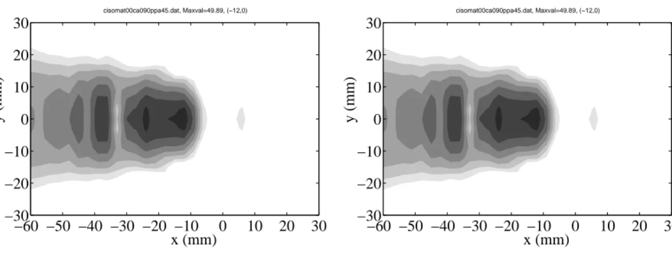
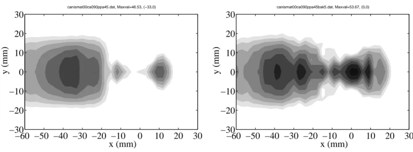
Next, the probe is changed to a 45o P probe and A-scans are given in Figs. 9−12 for both the isotropic and anisotropic austenite and both without and with a backside present. The crack is now vertical _{β = 90}o but the anisotropy is untilted _{γ = 0}o. On the isotropic austenite this probe sends out a P and an SV wave which correspond to maxima in the C-scan in Fig. 9 at x=−25 mm and x = _{−13 mm, respectively. The other maxima at larger negative x-values are due to} side lobes. With the backside present in Fig. 10 the signal becomes 18 dB stronger and this is of course due to the corner reflection between the crack and backside. On the anisotropic austenite the 45o P probe sends out a qP wave with an angle 50o and a qSV wave with an angle −23o _{and these correspond to maxima at x = −35 mm and x = 10 mm, respectively, in}

Fig. 11. It is noted that the P waves do not change very much between the isotropic and anisotropic cases whereas the changes for the SV waves are really profound. In Fig. 12 with the backside present the response again gets much stronger due to the corner effect and new maxima which are difficult to interpret appear.

cisomat00ca090ppa45.dat, Maxval=49.89, (−12,0) x (mm) y (mm) −60 −50 −40 −30 −20 −10 0 10 20 30 −30 −20 −10 0 10 20 30 cisomat00ca090ppa45.dat, Maxval=49.89, (−12,0) x (mm) y (mm) −60 −50 −40 −30 −20 −10 0 10 20 30 −30 −20 −10 0 10 20 30

Figure 9: C-scan for 45o P probe on the isotropic austenite with _{β = 90}o and _{γ = 0}o.

Figure 10: C-scan for 45o P probe on the isotropic austenite with _{β = 90}o, _{γ = 0}o and a backside.

12 canismat00ca090ppa45.dat, Maxval=46.53, (−33,0) x (mm) y (mm) −60 −50 −40 −30 −20 −10 0 10 20 30 −30 −20 −10 0 10 20 30 canismat00ca090ppa45bak5.dat, Maxval=53.67, (0,0) x (mm) y (mm) −60 −50 −40 −30 −20 −10 0 10 20 30 −30 −20 −10 0 10 20 30

Figure 11: C-scan for 45o P probe on the anisotropic austenite with _{β = 90}o and _{γ = 0}o.

Figure 12: C-scan for 45o P probe on the anisotropic austenite with _{β = 90}o, _{γ = 0}o and a back wall.

Figure 13 shows an A-scan from Fig. 11 taken at the maximum at x = −34 mm. The first strongest signal is of course the qP wave and it is seen that this is rather spread out, possibly due to a surface wave propagating across the crack. The later parts of the signal are qSV waves and these are much weaker and also more spread out in time.

0 5 10 15 20 25 30 35 40 −100 −80 −60 −40 −20 0 20 40 60 80 t (microsec) aanismat00ca090ppa45x−34

Figure 13: A-scan for 45o P probe on the anisotropic austenite with _{β = 90}o and _{γ =} 0o at the position x = _{−34 mm.}

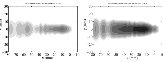
Figures 14−17 show results for a 60o _{SV probe on an isotropic and an anisotropic austenite}

and without and with a backside. The crack is still vertical and the anisotropy is untilted. Again the cases with a backside give a much stronger signal due to the corner effect. The anisotropic austenite gives somewhat more complicated results and the response is more spread out in the x direction.

cisomat00ca090spa60.dat, Maxval=45.16, (−41,0) x (mm) y (mm) −80 −70 −60 −50 −40 −30 −20 −10 0 10 −30 −20 −10 0 10 20 30 cisomat00ca090spa60bak5.dat, Maxval=62.18, (−35,0) x (mm) y (mm) −80 −70 −60 −50 −40 −30 −20 −10 0 10 −30 −20 −10 0 10 20 30

Figure 14: C-scan for 60o SV probe on the isotropic austenite with _{β = 90}o and _{γ = 0}o.

Figure 15: C-scan for 60o SV probe on the isotropic austenite with _{β = 90}o, _{γ = 0}o and a backside. canismat00ca090spa60.dat, Maxval=45.08, (−11,0) x (mm) y (mm) −80 −70 −60 −50 −40 −30 −20 −10 0 10 −30 −20 −10 0 10 20 30 canismat00ca090spa60bak5.dat, Maxval=58.47, (−14,0) x (mm) y (mm) −80 −70 −60 −50 −40 −30 −20 −10 0 10 −30 −20 −10 0 10 20 30

Figure 16: C-scan for 60o SV probe on the anisotropic austenite with _{β = 90}o and _{γ = 0}o.

Figure 17: C-scan for 60o SV probe on the anisotropic austenite with _{β = 90}o, _{γ = 0}o and a back wall.

4 Concluding remarks

This report has described work on a rectangular crack in an anisotropic component. Both the crack and the anisotropy may be arbitrarily oriented. The presence of a backside may be taken into account. One or two probes can be used, these are assumed to be of contact type but can otherwise be quite arbitrary. The main limitations are that the anisotropy is assumed

14

to illuminate the type of output that may be obtained. There are many parameters to vary so it is impossible to cover more than just a few variations in one or two parameters.

There is some follow-up work that would be worthwhile to do. One important thing is of course the validation of the present developments. This can be done with experiments, although there are a few difficulties with this. Firstly, it is not so easy to fabricate internal cracks that are smooth and with negligible distance between the crack faces. Secondly, it is not obvious what anisotropic material that should be used as it should be both homogeneous and thick-walled. Another way to make at least a partial validation is through comparisons with other mathematical models. As far as known there is a lack of other 3D models. EFIT may be a possibility, although it seems mostly to be restricted to 2D situations. But also a comparison with 2D could be worthwhile even though it would be hard do draw any definite conclusions about the absolute levels.

5 References

Boström, A., UTDefect _{− a computer program modelling ultrasonic NDT of cracks and other}

defects, SKI Report 95:53, Swedish Nuclear Power Inspectorate, Stockholm 1995.

Boström, A., Ultrasonic probe radiation and crack scattering in anisotropic media, SKI Report 97:27, Swedish Nuclear Power Inspectorate, Stockholm 1997.

Boström, A., Developments of UTDefect: rough rectangular cracks, anisotropy, etc, SKI Report 00:43, Swedish Nuclear Power Inspectorate, Stockholm 2000.

Boström, A., Grahn, T., and Niklasson, A.J., Scattering of elastic waves by a rectangular

crack in an anisotropic solid _{− modelling of ultrasonic nondestructive testing, Report in}

preparation 2001.

Boström, A., Grahn, T., and Niklasson, A.J., Scattering of elastic waves by a rectangular

crack in a thick-walled solid _{− modelling of ultrasonic nondestructive testing, Report in}

preparation 2001.

Boström, A., and Jansson, P.-Å., Developments of UTDefect: rough cracks and probe arrays, SKI Report 97:28, Swedish Nuclear Power Inspectorate, Stockholm 1997.

Eriksson, A.S., Boström, A., and Wirdelius, H., Experimental validation of UTDefect, SKI Report 97:3, Swedish Nuclear Power Inspectorate, Stockholm 1997.

Halkjaer, S., Elastic wave propagation in anisotropic, inhomogeneous materials _{− application}

to ultrasonic NDT, Thesis, Department of Mathematical Modelling, Technical University of

Denmark, Lyngby, Denmark 2000.

Hannemann, R., Modeling and imaging of elastodynamic wave fields in inhomogeneous

anisotropic media _{− an object-oriented approach, Thesis, Department of Electrical}

Niklasson, A.J., Elastic wave propagation in anisotropic media − application to ultrasonic

NDT, Thesis, Division of Mechanics, Chalmers University of Technology, Göteborg, Sweden